
Abstract
The aerodynamic and acoustic testing of a NACA0012 airfoil section was performed in an open wind tunnel, focusing on noise mechanisms at the trailing edge to identify and understand sources of noise production. The sound measurement profiles were captured by embedding microphones along the chord at various distances from the trailing edge and at different geometric angles of attack. The embedded microphones have successfully captured all noise sources due to aerodynamic flow over the NACA 0012 airfoil at the trailing edge, which included the following major peak frequencies: 44, 93, 166, and 332 Hz. The fundamental frequency of the model tested was identified by peak frequency (166 Hz). It appears that these frequencies do not deviate as the angle of attack is increased. The general trend is Strouhal numbers decrease as the flow moves downstream which indicates the amount of resonance (i.e. periodic, non-random vortices) decreases further downstream, which is to be expected given the onset of turbulence. Two bands of frequencies were identified. The frequency spectra between 1 and 3 kHz show a measure of far-field noise energy while frequency spectra in the range 3–10 kHz show near-field noise energy which is due to mechanisms associated with wake flow (separation).
Introduction
Knowledge of noise sources and mechanisms of noise production at the trailing edge (TE) of an airfoil are of great importance when considering the wing design of an aircraft. This is due to increased stringent limits and regulations imposed on allowed aircraft noise, and especially noise emitted on landing approach, a considerable source of noise pollution in airport neighboring communities. Design considerations to limit or reduce noise and vibrations have wide applications, such as in the wind turbine, airframe design, turbomachinery, ship hulls, and offshore structures’ industries.
Brooks et al. 1 have defined five airfoil self-generated noise mechanisms associated with subsonic flow surrounding an airfoil. One of these mechanisms pertinent to this study is broadband noise produced due to a turbulent boundary layer at the TE. This regime is due to flow at high Reynolds numbers, where the turbulent boundary layer development is maintained on most of the airfoil and the generation of broadband noise is due to turbulence that is convected over the TE. If the boundary layer separates, then in addition to the broadband noise, we experience several tonal peaks that are superimposed on the broadband noise; these narrow peaks perhaps are due to the vortex shedding at the TE associated with the flow separation.
It has been noted by Roger and Moreau 2 that an attached or separated turbulent boundary layer at the TE generates broadband noise; however, whistles are generated due to laminar boundary disturbances. In both scenarios, noise is generated due to vortical disturbances which are transformed into acoustical ones once they are convected downstream of the TE. This is defined as airfoil self-noise or TE noise. Roger and Moreau 3 described the self-noise production phenomenon as a balance of forces acting on eddies. Eddies transported downstream in the fluid are subjected to pressure gradients balanced by induced centrifugal forces. The source of the radiated noise is due to density variation that is induced by the thermodynamic gas properties’ changes caused by pressure variation due to inertia. The radiated noise is further intensified downstream due to the geometrical singularity at the TE as the flow is trying to adjust itself through rapid reorganization of the vortical structures.
Analytical analysis of airfoil self-noise generation followed mainly two stream of ideas, the first is of Ffowcs Williams and Hall. 4 Where the noise radiated by the vortical disturbances of the boundary layer downstream of the TE is related to the vortical velocity at the TE. Amiet 5 and Howe 6 introduced the second approach which relates the far-field acoustic signature statistics to the aerodynamic wall pressures’ statistics at some point upstream of the TE. Based on this methodology, the surface pressure is utilized as an equivalent acoustic source, although sound is generated due to the velocity field. The second approach has been implemented successfully by Brooks and Hodgson 7 and experimental support corroboration was reported by Brooks et al. 1 and Roger and Moreau. 3
Experimental apparatus and acoustics measurements
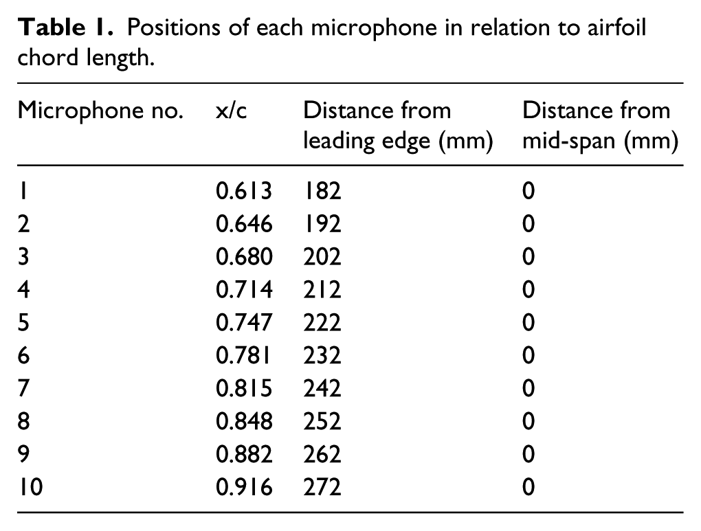
A physical NACA0012 airfoil model, shown in Figure 1, was fabricated comprising several components, each requiring different manufacturing processes. The airfoil itself was made of two components, the upper surface and lower surface, and was three-dimensional (3D) printed using information from computer-aided design (CAD) files exported to a format based on a coordinate system, which the 3D printer could read (they are made from a plastic material called acrylonitrile butadiene styrene, ABS in short). This airfoil has a chord length of 297 mm and a maximum thickness of 35.6 mm and includes ten 0.4-mm-diameter pinholes for the location of interior microphones, the exact locations of which are documented in Table 1. The airfoil is 150 mm in width. Calculations based on the new chord length were made, which enabled the placement of pinholes such that they would be near enough to the TE to experience the effects of turbulence. Designing the airfoil proved to be challenging given the narrow dimensioning near the TE; however, the 10 microphones were successfully placed as near as was possible to the TE while maintaining the external profile. The microphones used were “Kingstate KECG2740PBJ Electret Condenser Microphones,” which have a diameter of 6 mm and a 5.5-mm height, including terminal pins. The two terminals of the microphones essentially have one terminal for the signal output (the data), which was passed through a 0.1-µF capacitor and 2.2-kΩ resistor, and another terminal to ground the system. A single wire carried the power supply output, which fed a signal of 2.5 V to each microphone. During the experiment in the wind tunnel, each of these wires was probed using a two-channel “PicoScope” 5203 series Oscilloscope, 8 which was able to display signal data via software on a computer. The sampling rate was 40,000 samples per second.
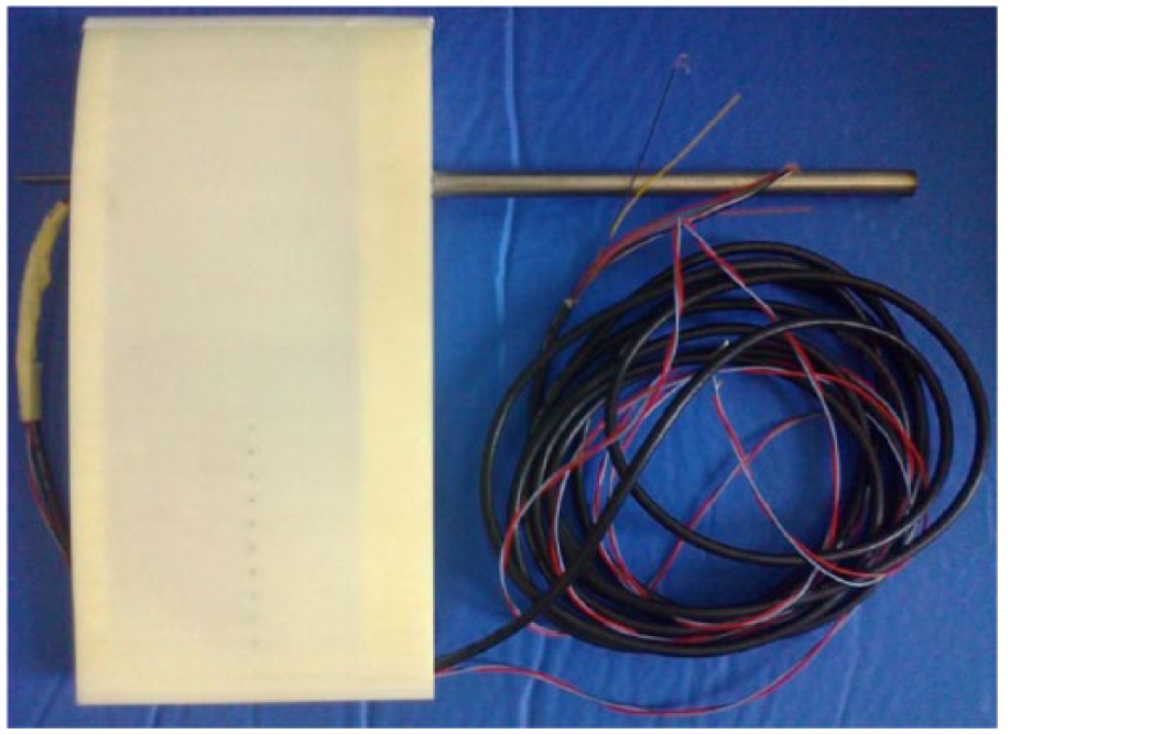
Top view of NACA0012 final model, as tested in the wind tunnel.
Positions of each microphone in relation to airfoil chord length.
As indicated by the model calculations, the experiment for acoustic analysis was tested at 20 m/s, with a Reynolds number (based on chord) of 406,849, sufficient to cause turbulence effects, and at angles of attack (AoAs) of 0°, 4°, 8°, 12°, and 16°. A low-pass filter was used to cut off frequencies higher than 20 kHz.
Acoustic data analysis
Calculations based on the new chord length of the scaled model show that at a free-stream velocity of 20 m/s, in level flight and for the chord length of the test model, a turbulent boundary layer is likely to develop past 37% of the overall linear chord length, and so the chosen microphone pinhole locations (shown in Table 1) are sufficient to capture turbulent effects. Figure 2 shows the location of these pinholes on the model itself. A side view is also shown for clarity in Figure 3.
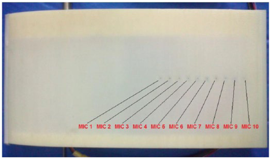
Microphone location: the coordinate system indicated in Table 7 has its origin at the leading edge-mid span of the airfoil.
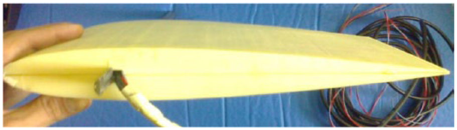
Side view of the produced airfoil model.
Careful analysis of the frequency spectra for each individual microphone has enabled the collation of the data presented in Tables 2–5. Representative spectrum plots for microphones 1 and 2 at 0° AoA are given in Figures 4 and 5, respectively. The frequency measurements are plotted logarithmically, as is the convention, since this enables a clearer perspective of the patterns and trends between curves. The sampling rate of the oscilloscope was 40,000 Hz, although as mentioned a low-pass filter was used to measure activity below 20,000 Hz. In all, 4096 samples were plotted and an averaging method was used to plot the root mean square (RMS) value of dBu. Note that the value of dBu gives a relative measure of noise to the “unloaded” reference level of the input voltage (hence the suffix “u”). This means that the higher the pressure induced by noise, the more attenuation is applied via the microphone to the individual microphone’s voltage supply. Essentially, this information is relayed back through the data channel, and hence, it is the reduction in voltage compared with the original input, which gives a measure of relative decibel between frequencies. This is also the reason that the dBu values are negative (the more negative, the less the perceived volume).
Results of acoustic spectrum analysis for 0°.
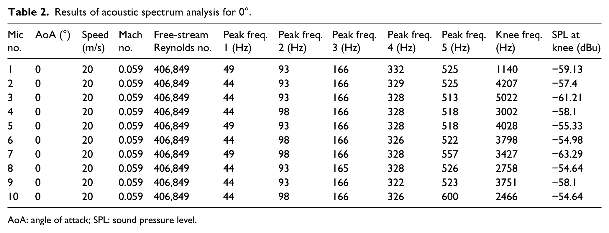
AoA: angle of attack; SPL: sound pressure level.
Results of acoustic spectrum analysis for 4°.
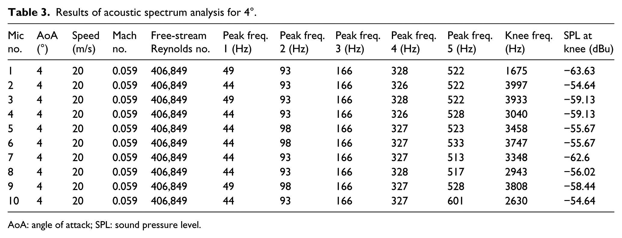
AoA: angle of attack; SPL: sound pressure level.
Results of acoustic spectrum analysis for 8°.
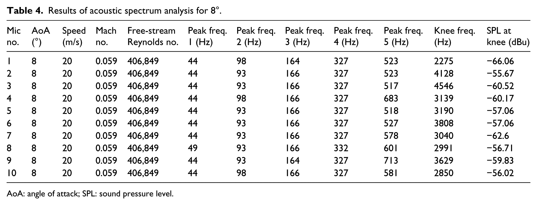
AoA: angle of attack; SPL: sound pressure level.
Results of acoustic spectrum analysis for 16°.
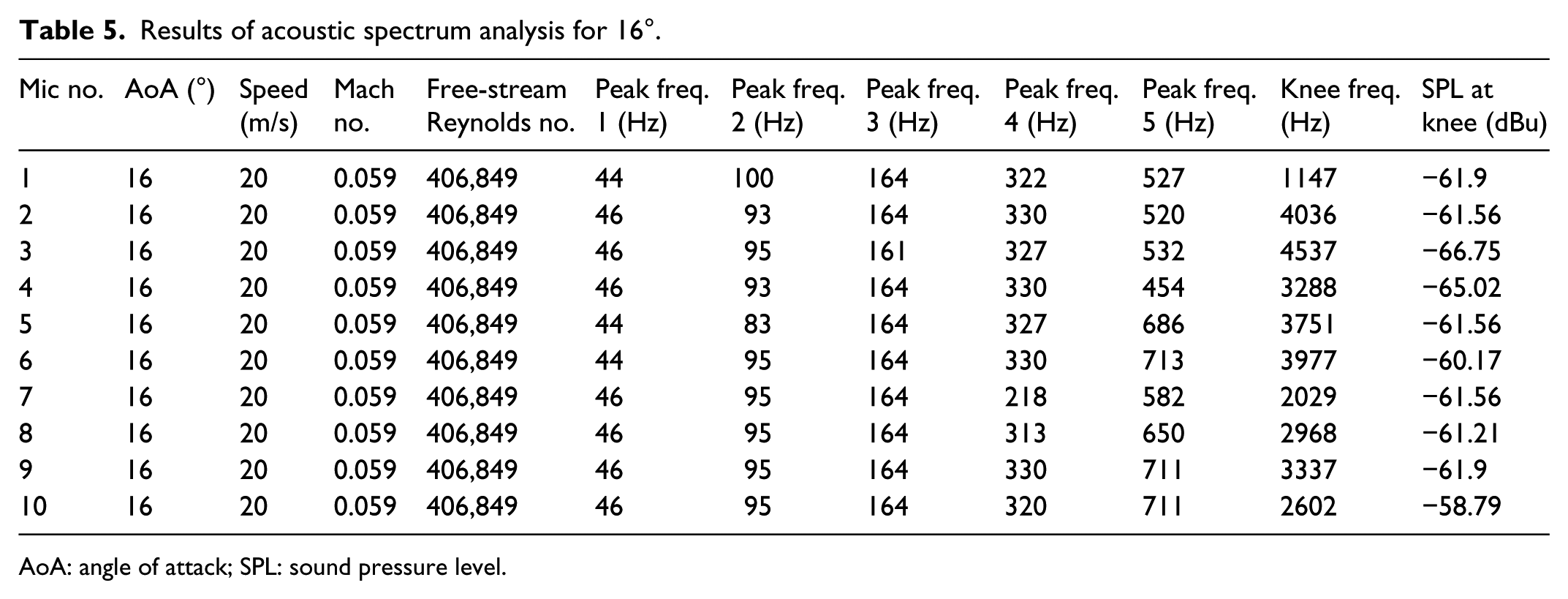
AoA: angle of attack; SPL: sound pressure level.
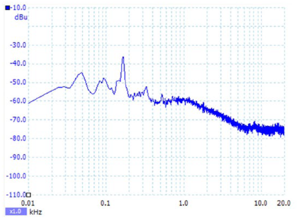
dBu versus frequency, microphone 1, AoA = 0.
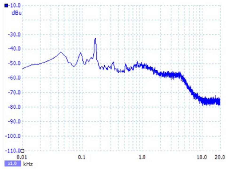
dBu versus frequency, microphone 2, AoA = 0.
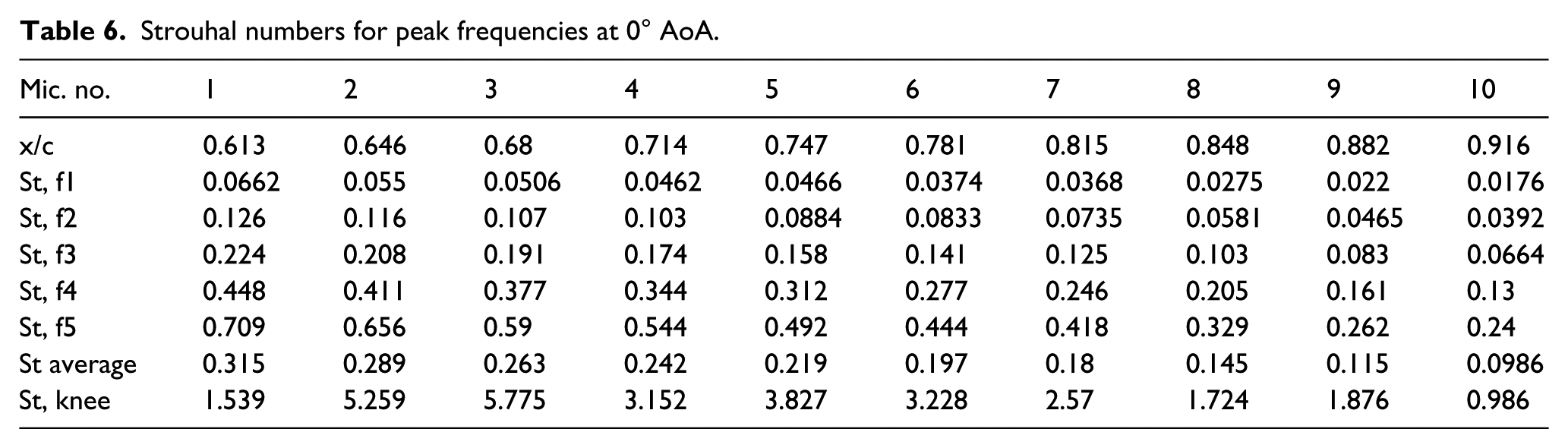
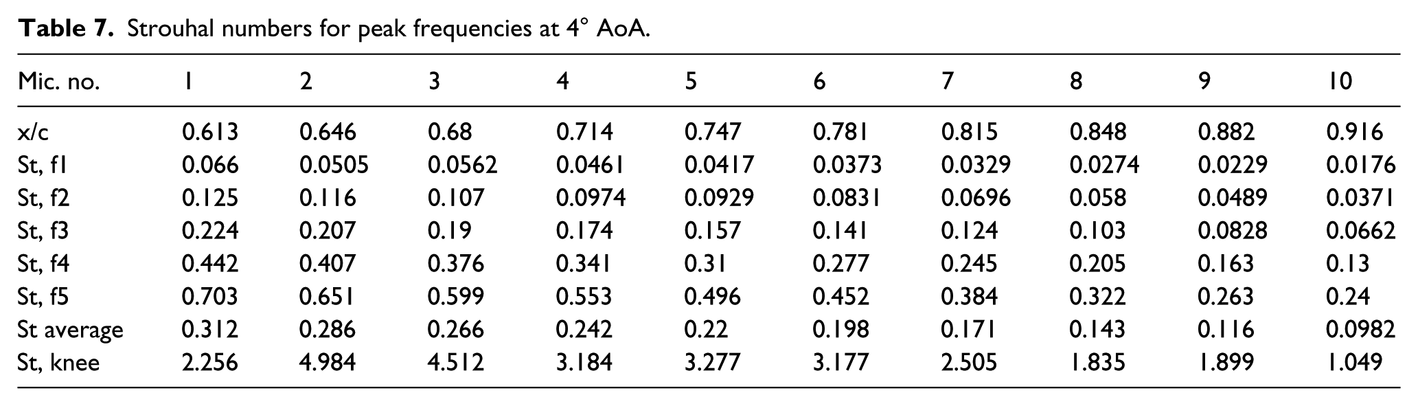
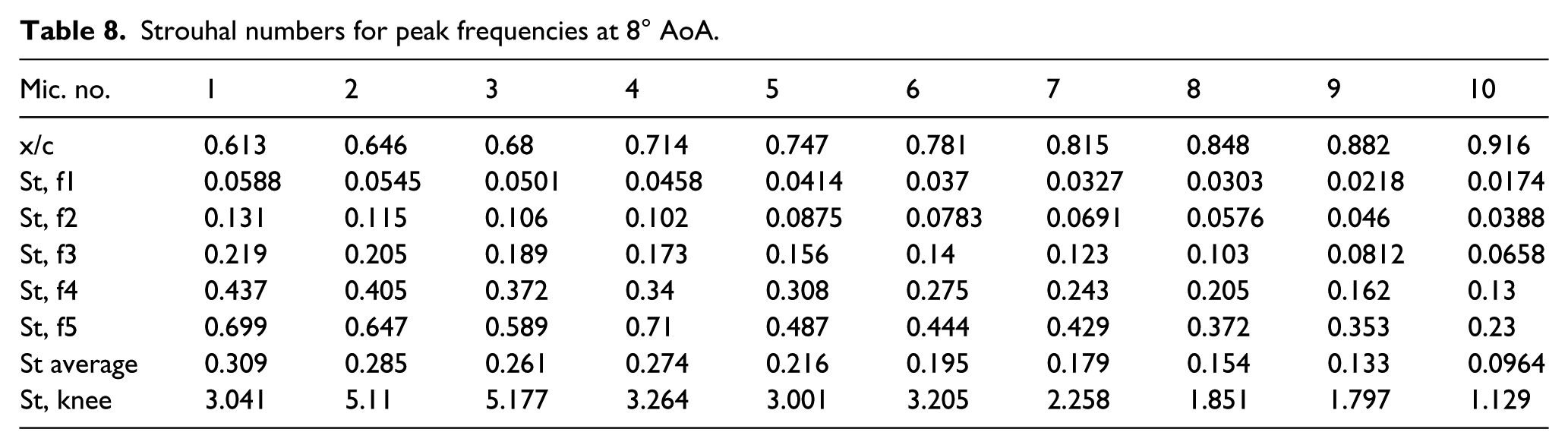
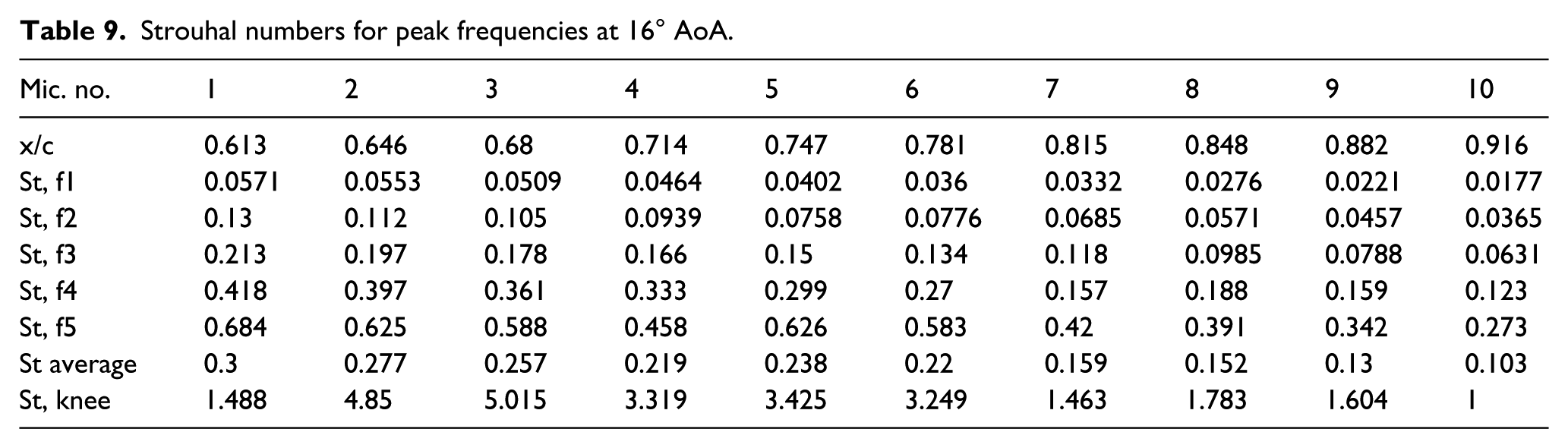
The spectra suggest some interesting developments which will be discussed in detail later. In general, the most dominant activity relating to noise contribution with regard to airflow around the airfoil happens in the regions around 200–7000 Hz. It is suggested that the most revealing area for investigation into aero-acoustic noise concerned with the NACA 0012 model begins at around 500–1000 Hz, when the curves become less erratic and display an interesting change in gradient toward the latter part of the spectra, which levels out again at around 10,000 Hz. Since all the spectra show loud (bass/low-mid) peaks at around 44, 93, and 166 Hz, and a similarly less dominant peak at around 327–330 Hz, it may be that one or more of these frequencies is due to the wind tunnel fan (which ran constantly at the same speed), but the majority of these peaks could also be due to surface flow phenomena entirely related to the experimental model; information from experimental sources provided during validation will explain the reasons for such peaks. The changes in gradients observed have been plotted for closer inspection between 1000 and 10,000 Hz for mic. numbers 1, 5, and 10 in Figures 6–9. Tables 6–9 present data from calculations of Strouhal number (see Appendix 1) for various peak frequencies. Graphs are given in Figure 10 that plot these Strouhal numbers against chord length percentage (x/c), for visual understanding of turbulence and vortex shedding phenomena.
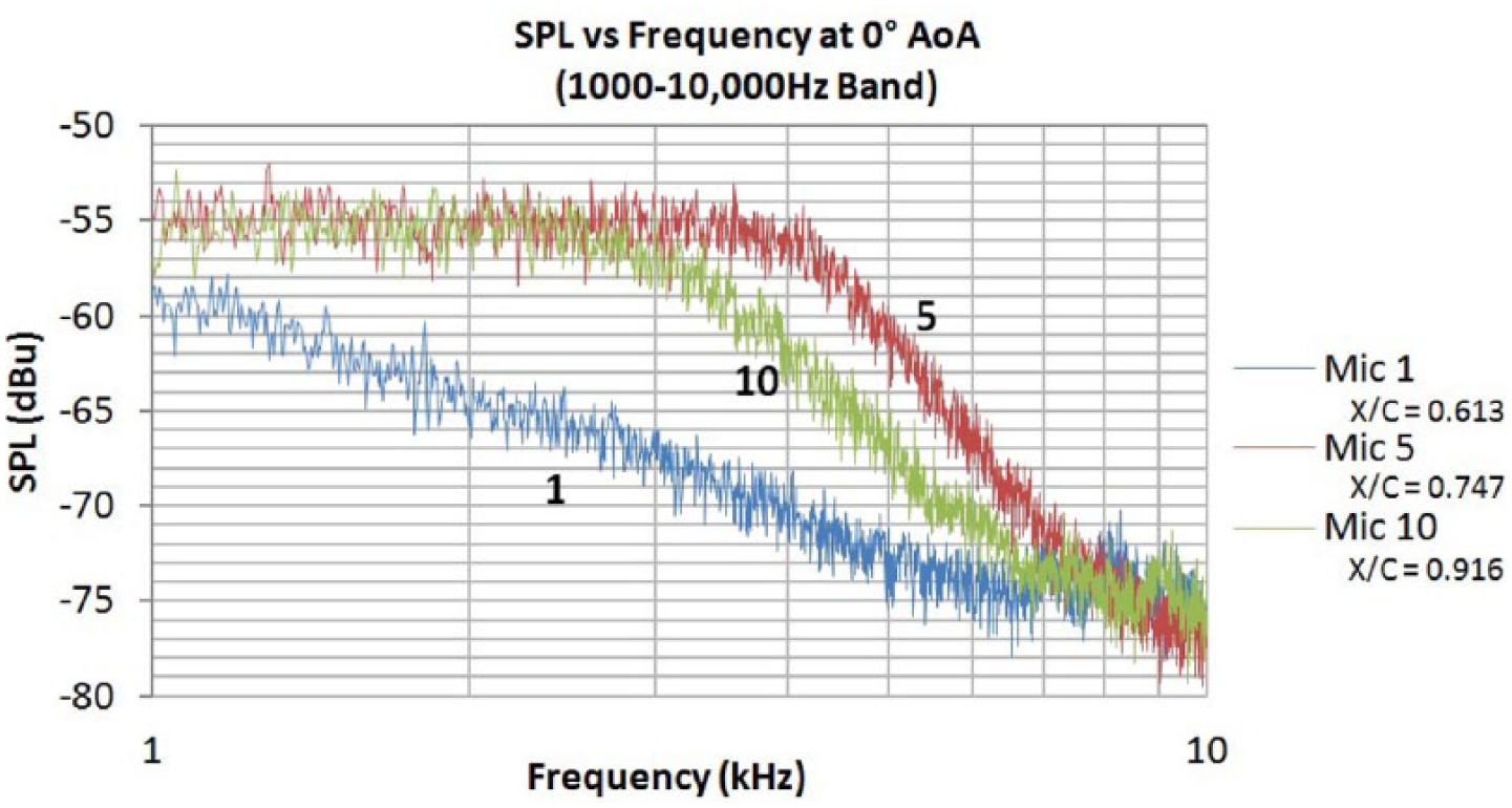
Frequency as a function of dBu at 0°.
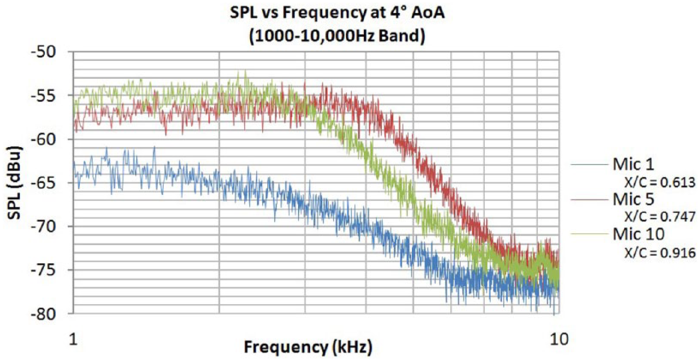
Frequency as a function of dBu at 4°.
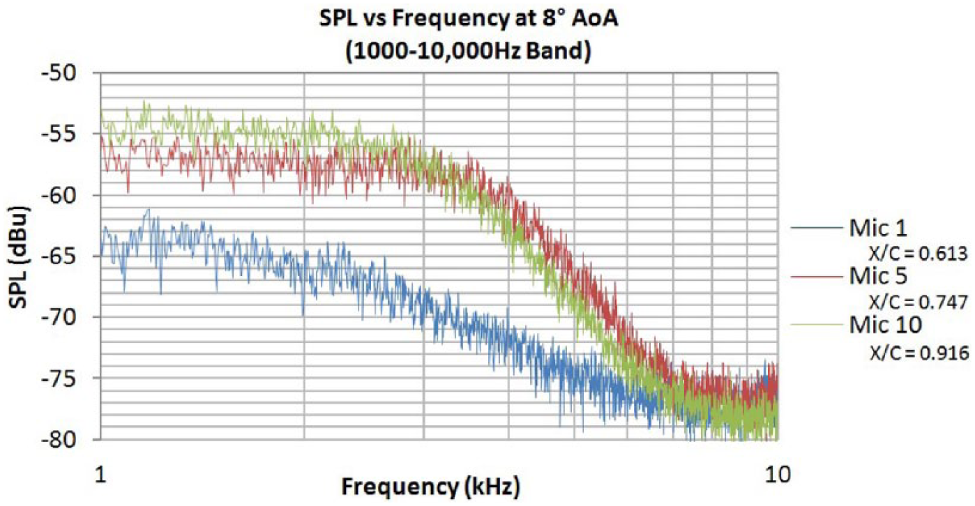
Frequency as a function of dBu at 8°.
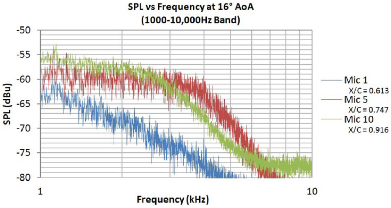
Frequency as a function of dBu at 16°.
Strouhal numbers for peak frequencies at 0° AoA.
Strouhal numbers for peak frequencies at 4° AoA.
Strouhal numbers for peak frequencies at 8° AoA.
Strouhal numbers for peak frequencies at 16° AoA.
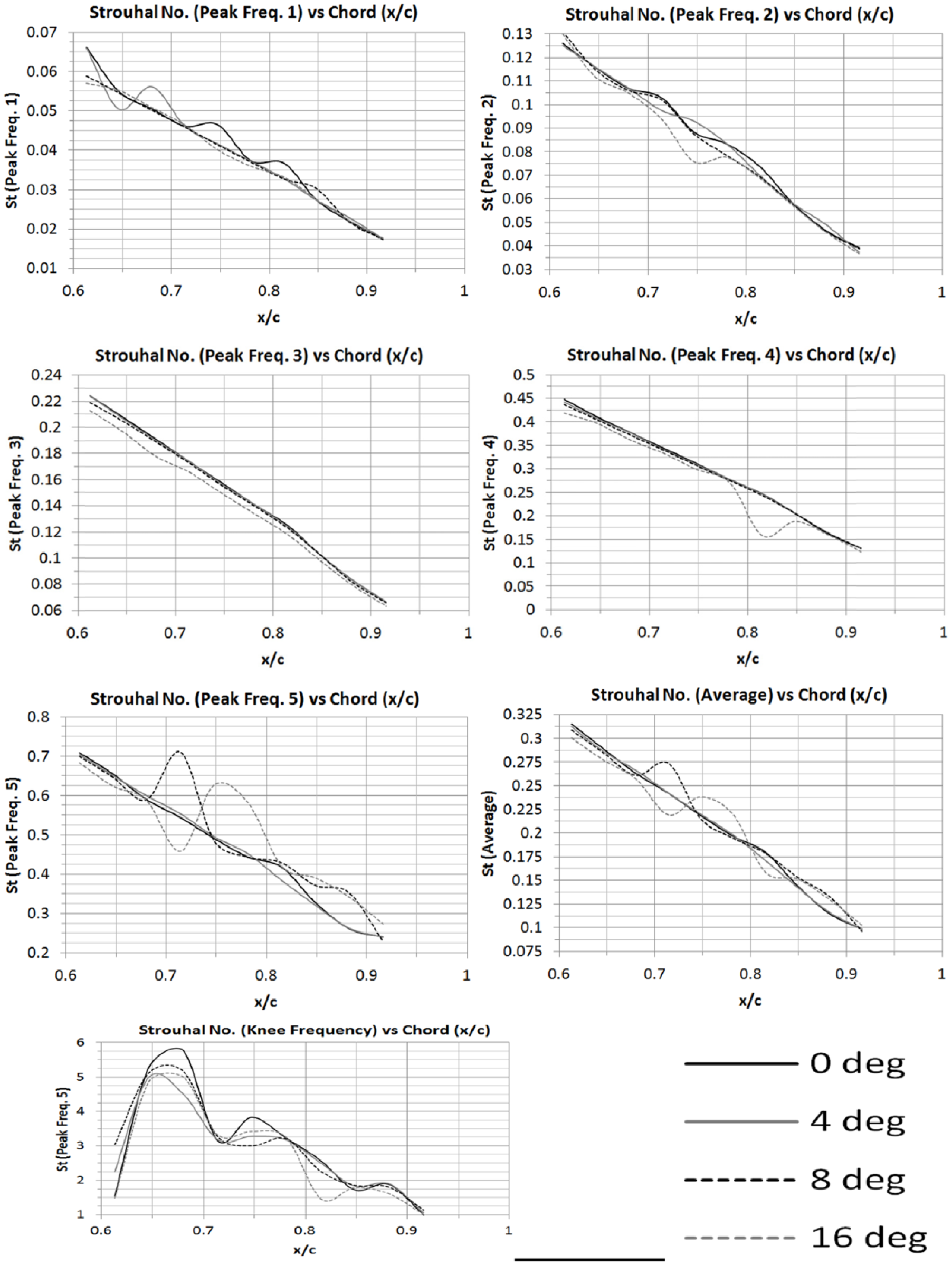
Strouhal number at different peak frequencies versus chord length.
Validation
Considering the complexity of the experiment, the observed results have in fact correlated well with the existing data. Considered validation data include the energy/frequency spectra (as mentioned previously, the sound pressure level is effectively a measure of the noise energy), the calculated values for boundary layer parameters and skin friction, and also the existing data for Strouhal number calculations on similar experiments.
Energy/frequency spectra
When reviewing the energy/frequency spectra of similar experiments, it has become clear that the experiment performed in this research has captured noise mechanisms related to the NACA 0012 airfoil to a significant level. This is demonstrated through the comparison of the current results to Garcia-Sagrado and Hynes, 9 in which tests were performed with lower Reynolds numbers. Although the comparison has a lower Reynolds number than the one tested presently, the results are strikingly similar. For example, there are dominant peaks in frequency at around 190 Hz and also at around 380 Hz. A similar observation can be made from the noise spectra, where these two early dominant peaks correspond to around 44 and 166 Hz.
Toward the TE, overall noise (or energy) is seen to reduce, which is also what has been observed in the spectra for this experiment, albeit scaled differently; in the region of around 200–1000 Hz, a reduction in pressure level can be seen. This is in agreement with the report by Garcia-Sagrado and Hynes, 9 which included spectra for a Reynolds number of 200,000 and 400,000, with altered AoAs of 12.6° and 16°. It is interesting to note the decay of the slope in each graph; it appears that at the TE, for smaller frequencies, the energy is relatively lower initially (compared with the leading edge), whereas past a certain point, noise energy toward the TE is lost at a faster rate (most spectral plots cross paths) than at the leading edge. It also appears that for the Reynolds number of 400,000, the total spectral energy is higher as the AoA is increased from 12.6° to 16°. Excluding microphone 1 in this experiment, the spectral plots of microphones 5 and 10 in Figures 6–9 show just this phenomenon, which would suggest that the experiment has been successfully performed, and valid results have been obtained for this situation.
Furthermore, it is stated that for shear noise layers, the slopes of the noise spectra decay after a “broad” peak, 10 which varies with fn where n = 1.5–2.0, since the slope decay after the peak frequency is not universal (as is observed by different airfoil positions, AoAs and Reynolds numbers).
Boundary layer and skin friction values
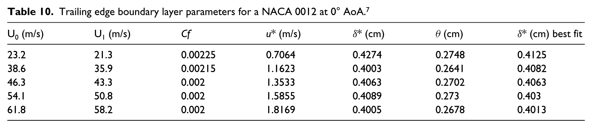
Comparing Table 10 with the experimental data by Brooks and Hodgson, 7 it can be seen that the orders of magnitude of the skin friction coefficient (at 23.2 m/s free-stream velocity) are similar to those calculated and presented in Table 11. At 20% chord, the laminar skin friction coefficient was calculated to be 0.00233, similar to those in Table 10.
Trailing edge boundary layer parameters for a NACA 0012 at 0° AoA. 7
Surface parameters dependent on chord-wise location (level flight).
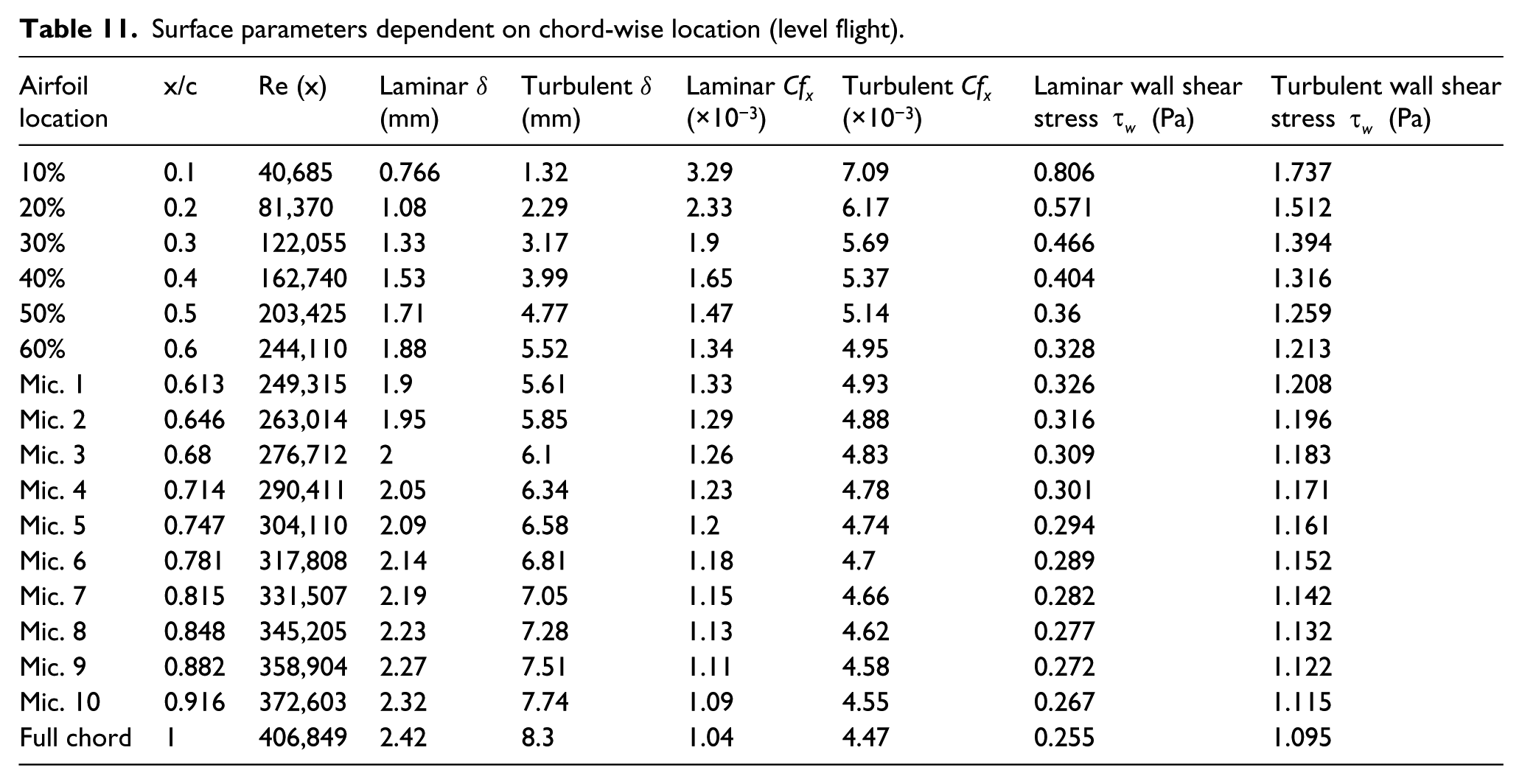
Depending on whether flow is laminar or turbulent, the boundary layer thickness was calculated to be within around 1–8 mm (0.1–0.8 cm), a similar order of magnitude to the displacement thickness given in Table 10 by Brooks and Hodgson; 11 due to the fact that the velocity increases asymptotically from the airfoil surface up until reaching free-stream velocity, displacement thickness (δ*) is effectively a measure of boundary layer thickness, but scaled as if the flow were inviscid. Also, as the speed is increased (represented by the Reynolds number in Table 11), the value of skin friction coefficient decreases, as observed in Table 11. Thus, the recorded data for this experiment appear to be valid.
Strouhal values
Figures 11 and 12 show plot points of peak frequency Strouhal numbers calculated in the experiments by Brooks et al. 1 using a NACA 0012 airfoil, with the minimum tested speed being 31.7 m/s, and with AoAs of between 0° and 25.2°. Figure 11 gives the plots for a laminar boundary layer, whereas Figure 12 gives the plots for a turbulent boundary layer. Although the data are for a slightly higher speed, it is clear that the Strouhal numbers calculated for various peak frequencies (Tables 6–9) would fit within the same magnitude. For a laminar boundary layer, the peak Strouhal numbers appear to lie within around 0.18–0.3, whereas they lie within 0.04–0.5 for a turbulent boundary layer. In general, for a laminar boundary layer, they also appear to decrease in magnitude with AoA, whereas under a turbulent boundary layer the Strouhal numbers increase in magnitude with AoA. Looking at the plotted Strouhal numbers in Figure 10(a)–(g), this would suggest that along some parts of the airfoil, there may be re-laminarization of the turbulent boundary layer; however, the Strouhal numbers do show this trend in Figure 10(e) (peak frequency 5) and Figure 10(f) (Strouhal number averages) at the airfoil chord length (x/c) of about 0.84 onward.
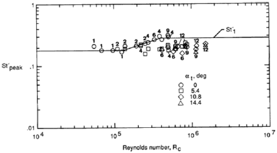
Laminar boundary layer (LBL) peak Strouhal numbers versus Reynolds number. Numbers represent chord size in inches. 1
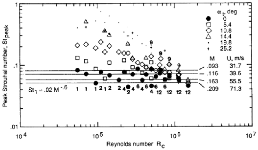
Turbulent boundary layer (TBL) peak Strouhal numbers versus Reynolds number. Numbers represent chord size in inches. 1
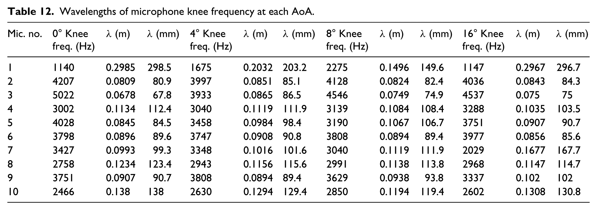
Since many calculations have been performed for each microphone and at each AoA, a large amount of data have been collected (much is given in Tables 6–13); for conciseness, example calculations are given in Appendix 1 for data at 20% chord (x/c = 0.2) and microphones 1and 10. In the case of Strouhal numbers, example calculations are given for peak frequency 5 at 16° AoA and for microphone 1. Tables 11–13 summarize the data for all points.
Wavelengths of microphone knee frequency at each AoA.
Noise intensity and OASPL with comparison of the average knee noise level.
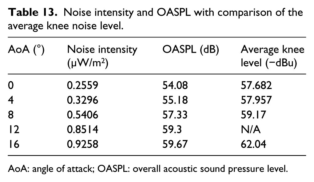
AoA: angle of attack; OASPL: overall acoustic sound pressure level.
Chord length points (X) and trailing edge thicknesses.
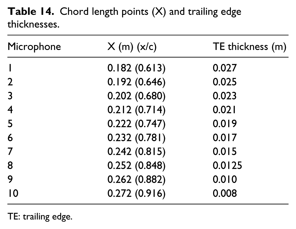
TE: trailing edge.
Results
First, looking at Tables 8–11, it is interesting to note that the first four peak frequencies do not deviate significantly between measurements at each AoA (they are 44, 93, 166, and 332 Hz approximately). It was at first thought that these peaks may have been related to the mechanisms of the wind tunnel fan; however, given that these results are very similar in form to those reported by Garcia-Sagrado and Hynes 12 (who included measures to reduce fan noise), it is suggested that these peak frequencies arise due to the generation of vortical structures such as described in the introduction. A revealing observation is the fact that using the wave equation to determine the second harmonic of the frequency peak at 166 Hz in fact gives a value of 332 Hz (peak frequency 4), whereas the first, fifth, and “knee” frequencies are not related harmonically, and so must be related to the behavior of the flow itself, or due to shear interactions between the flow and the airfoil surface. Thus, it can be deduced that the embedded microphones have successfully captured all noise sources due to aerodynamic flow over the NACA 0012 airfoil at the TE—and the fundamental frequency of the model is therefore given by peak frequency 3 (166 Hz). The second harmonic frequency of the fundamental frequency has been identified. Observing the noise spectrum plots revealed reduction in the energy as the AoA increased. This can be explained by the initial propagation of Tollmien–Schlichting waves. The initial wavelength can be determined by the fundamental/natural frequency the NACA0012 model resonates at. This is therefore an indication of laminar boundary layer vortex shedding noise. Further downstream, the second harmonic is less pronounced, and so it can be inferred that the Tollmien–Schlichting waves have become much more unstable, and consequentially, other noise mechanisms dominate, which must relate more to turbulent TE noise.
At this point, much can be inferred from the gradients of the frequency spectra in the range of around 1–10 kHz, as presented in Figures 6–9 (for microphones 1, 5, and 10). Some particularly telling observations are the steepening of the slope with an increase in AoA for microphone 1, and also the decay of the slopes of microphones 5 and 10. These observations could also be related to the steepening and magnitude of the adverse pressure gradient and would suggest that for a given point (or microphone location), for different AoAs, vortices are at different stages of development. Since there is more turbulence within the boundary layer at the same chord-wise point for an increased AoA, it is posited that the shape and gradient of the slopes given in Figures 6–9 are determined by the onset of Kelvin–Helmholtz instabilities.
This is attributed to the fact that at lower AoA, for the same location, a higher proportion of higher frequencies is observed than at higher AoAs. This can be explained by less time the Kelvin–Helmholtz instabilities have had to dissipate. Therefore, vortices are smaller at such point which result in shorter wavelength, and hence, higher frequencies are observed. This theory is further supported by the fact that plotted Strouhal numbers (see Figure 10) appear to have significant variation at the higher frequencies of peak frequency 5 and also at the knee frequency, which is the frequency measured at the point just before the slope begins to decay linearly. This is in contrast to peak frequencies 3 and 4. This means that there are more inherent turbulent mechanisms at the higher frequencies (such as the mixing of flow due to Kelvin–Helmholtz instabilities). At the same time, the general trend is for the Strouhal number to decrease as flow moves further downstream, meaning that the amount of resonance (i.e. periodic, non-random vortices) decreases further downstream, which is to be expected given the onset of turbulence.
Another interesting observation (Figures 6–9) is the fact that the sound pressure level at microphone 10 appears to decay sooner than microphone 5, within the region of 3–10 kHz, yet is still always significantly higher in magnitude to microphone 1. This decay of microphone 10 seems to come closer to replicating that of microphone 5 as AoA is increased; yet looking closely at the frequency range of 1–3 kHz, the increase in sound pressure level of microphone 10 over microphone 5 can be seen. Essentially, there is a crossover point between these regions which appears to happen earlier as AoA is increased. Since it has been established that Kelvin–Helmholtz instabilities are thought to play a key role in the profile of these gradients, this would suggest that there is in fact a higher amount of turbulent energy at microphone 5 in the region of about 3–10 kHz, than there is at microphone 10, for lower AoAs. Consider that microphone 1 could always be in a region which experiences similar, viscous flow behavior (less unstable), whereas if the flow is more turbulent downstream at microphones 5 and 10, it would make sense to observe a higher proportion of higher frequencies, which is the case. When the frequencies are broken down further into the bands between 1–3 and 3–10 kHz, however, further hypotheses can be made.
Between 1 and 3 kHz, a suggestion is that the frequency spectra show a measure of the far-field noise energy. Microphone 1 measures less energy in this portion because the boundary layer is still relatively small; effectively it may be measuring the free-stream flow energy outside of the boundary layer. Whereas microphones 5 and 10 are actually measuring energy within the boundary layer, as it has grown to a sufficient size at this point. It is worth noting microphone 5 detects the turbulent energy slightly closer to the outer edge of the boundary layer than does microphone 10, which measures a higher turbulent energy.
On the other hand, between 3 and 10 kHz, a phenomenon which would explain the differences in slope at microphones 5 and 10 is separation stall noise. As AoA is increased, the boundary layer at microphone 10 has a much higher affinity to separate (higher local Reynolds number) than microphone 5 (and microphone 1). Therefore, within the near-field region, there is less energy due to small-scale vortical formations than there is at microphone 5, and effectively, the only noise energy being measured is due to the back-draft of wake flow. This also explains why the slope of microphone 10 becomes closer to microphone 5 as AoA is increased, since microphone 5 is also beginning to detect noise mechanisms due to wake flow. This theory is also supported by the calculations of boundary layer thickness, skin friction, and wall shear stress (see Table 11), which show that viscous forces do in fact reduce with location along the TE.
As previously mentioned, a probable source of error in the acoustic testing was considered to be the fan blades which drive the wind tunnel. However, as this source has been deemed insignificant with relation to the actual shape of the energy/frequency spectra, the only deviation of measurements due to this source could be the overall magnitude of the sound pressure level. Given that the most important factor in determining how noise phenomena interact at the TE is the shape and characteristic peaks of the spectra, and how they relate to each AoA, this potential source of error is largely irrelevant since the research set out to understand noise mechanisms, first and foremost, rather than deriving a universal sound level.
Another source of error which may have affected the results portrayed by the acoustic testing is the surface roughness of the airfoil model. Validation data of similar experiments such as by Garcia-Sagrado and Hynes 12 used an airfoil with a very smooth surface, whereas due to the limits of the 3D printing mechanism used, the produced airfoil model had a slightly higher surface roughness. This explains why the spectra given as validation data appear to decay sooner (or at least with steeper gradient), as there is less near-field turbulence associated with the surface roughness.
A final source of error is the fact that the microphones used have their own frequency response, which is inevitably slightly different than the frequency response of the microphones used in similar experiments. However, this response only affects results past 10 kHz, which was considered during testing, and hence why measurements were plotted up to 10 kHz.
Conclusion
Airfoil self-noise or TE noise was investigated experimentally using an open subsonic wind tunnel focusing on noise mechanisms at the TE to identify and better understand sources of noise production. This is essential to mitigate the acoustic scatter through better design of airfoils for various applications in the aircraft and marine industry. The sound measurement profiles were captured by embedding microphones along the chord at various distances from the TE and at different geometric AoAs. The embedded microphones have successfully captured all noise sources due to aerodynamic flow over the NACA 0012 airfoil at the TE, which included major peak frequencies at 44, 93, 166, and 332 Hz. The fundamental frequency of the model tested was identified by peak frequency (166 Hz). It appears that these frequencies do not deviate as the AoA is increased. The general trend is that Strouhal numbers decrease as the flow moves downstream, which indicates that the amount of resonance (i.e. periodic, non-random vortices) decreases further downstream, which is to be expected given the onset of turbulence. Two bands of frequencies were identified. The frequency spectra between 1 and 3 kHz show a measure of far-field noise energy while frequency spectra in the range 3–10 kHz show near-field noise energy, which is due to mechanisms associated with wake flow (separation).
Footnotes
Appendix 1
Acknowledgements
The research was conducted by B.R.J. in partial fulfillment of BSc (Hons) in Aerospace Technology at the Department of Engineering and Math at Sheffield Hallam University under the supervision of S.M.D.
Declaration of conflicting interests
The author(s) declared no potential conflicts of interest with respect to the research, authorship, and/or publication of this article.
Funding
The author(s) received no financial support for the research, authorship, and/or publication of this article.