
Abstract
In recent years, magnetorheological dampers (MRD) have played a significant role in vibration control in various fields such as vehicles, military, building structures, etc. However, the mechanical model of MRD is very complex due to its hysteresis, which makes it difficult to identify the model’s parameters. In addition to experimental data, under the condition of no other prior knowledge, eight unknown parameters of the Bouc-Wen model are identified in this study based on the particle swarm optimization (PSO) algorithm. According to the trend of parameter variation with current, fitting research is conducted, and the variation law of parameters with current is summarized. Based on the identified parameters, the MRD’s output force is predicted under any current other than the experimental current. Subsequently, the application of MRD in semi-active control of power equipment is performed out, and proposed Simulink calculation programs for single-stage and two-stage vibration control systems are built. Then, a comparative study with passive and active control is conducted. In this paper, linear quadratic regulator (LQR) control is adopted for the active control, and the controller’s parameters are optimized based on the PSO algorithm. The results show that the adopted semi-active control can significantly reduce the transmitted force from power equipment to the foundation and can effectively mitigate the disturbance of power equipment to the environment. This study offers important guidance for the vibration control of MRD in industrial engineering.
Keywords
Introduction
Power equipment includes large-scale slewing, reciprocating, impact, and random vibration devices, all of which play pivotal roles in the national economy and defense construction. However, the generated vibration during their operation causes damage to the equipment itself and harms the operators, industrial buildings, and the surrounding environment. Taking effective isolation, vibration reduction, or vibration control measures can reduce the vibration of the power equipment itself and mitigate the adverse effects of the generated vibration on the surrounding environment.
The passive control system does not consider external energy input and does not rely on other automatic control systems. When the system is designed, the structural parameters are fixed, and the damping and stiffness are not adjustable, consequently, it cannot fully adapt to a wide frequency band. As a result, a poor isolation effect often does not reach the expected level and cannot adaptively adjust external interference changes, including amplitude changes, frequency changes, or changes in excitations’ form.1–3 In this case, active control methods become a viable alternative.
Active control methods encompass proportional integral differential (PID) control, 4 linear quadratic regulator (LQR 5 ) control, linear quadratic Gaussian (LQG 6 ) control, and H2/H∞ control. 7 The above methods have certain requirements for establishing accurate computational models, such as transfer function models or state-space models. However, this type of methods has certain limitations when there is uncertainty in the mass, stiffness, or damping of the vibration system or when the system has strong nonlinearity. 8 Therefore, many scholars have conducted research on intelligent control methods, such as fuzzy logic control (FLC), 9 neural network control (NNC), 10 and fuzzy neural network control (FNNC). 11 The above control methods have been widely applied in vibration control fields such as vehicle vibration reduction, structural seismic resistance, and structural wind resistance.12–14
In active control strategies, the actuator output is high, and the control effect is good. However, there are some drawbacks, such as complex sensor/actuator system and inconvenient vibration data acquisition and processing processes. Moreover, significant control energy should be consumed, bringing adverse economic effects. In addition, active control systems often inevitably have time delay, potentially diminishing the vibration control effectiveness and even causing response divergence when the delay is considerable.8,15,16 For this reason, scholars have proposed a semi-active control method that falls between passive control and active control. This method only requires a small amount of energy to maintain the normal operation of electronic and electrical components and does not require external energy to directly provide control force, thus eliminating the need for devices that apply control force and energy devices that support active control work. 17 Semi-active control mainly includes semi-active variable stiffness control18,19 and semi-active variable damping control.20–22
With the emergence of smart materials and smart dampers in recent years, traditional semi-active control technology has been greatly innovated and promoted. Electrorheology damper (ERD) represents a new type of damper based on electrorheology fluid (ERF) where in the damping viscosity can vary with the strength of the applied electric field. In the absence of an electric field, the ERF flows freely. When the applied electric field reaches a certain value, the ERF becomes gel instantly, and the response gets reversible within milliseconds.23,24 Wang et al. 25 applied ERD to the semi-active control of structures, and Choi 26 applied ERD to the study of the semi-active control of fixed beam structures.
Shortly after the invention of ERD, scientists discovered magnetorheological fluid (MRF), and based on this, MRD was invented. Compared with ERF, MRF offers significant advantages
8
such as: 1.The driving voltage of ERF is large, generally up to several thousand volts, while MRF only has a few volts to tens of volts. 2.The shear strength of MRF is much greater than that of ERF, resulting in MRF being significantly smaller in volume, generally 100∼1000 times smaller than that of ERF. 3.MRF is not sensitive to impurities in the body and has a wider temperature adaptation range.
In recent years, many scholars have applied MRD to semi-active control fields such as military, industrial, and civilian applications.27–30
Due to the special mechanical hysteresis properties of MRDs, 31 their mechanical models are very complex, posing challenges in parameter identification. The Bouc-Wen model is the most typical one, and Ikhouane et al.32,33 used analytical methods to provide a detailed explanation of the parameter identification process of this model. However, its parameter identification process was exceptionally complex and required many assumptions and definitions. Giucelea et al.34,35 employed the genetic algorithm (GA) to identify the parameters of the Bouc-Wen modified model. Nevertheless, this study assumed that four unknown parameters are constant or that the model’s expression should be modified. Therefore, under the condition of no prior knowledge other than experimental data, how to identify the parameters of the Bouc-Wen model through non-analytical methods has become a research focus.
The introduction of GA has addressed engineering optimization problems in multiple fields. However, its optimization ability is significantly insufficient when there are optimization objects with high recognition as the goal, when parameters to be optimized have high correlation, and when the dimension of optimization parameters is large. To overcome these shortcomings, Eberhart and Kennedy firstly proposed a new swarm intelligence optimization algorithm called the particle swarm optimization (PSO) algorithm in 1995. 36 The main idea was to find the optimal solution (particle) through cooperation and competition among particles. Renowned for its simplicity, easy implementation, fast convergence, and few adjustable parameters, this algorithm has been widely used in optimization calculations in the engineering field.37,38
In this study, the authors aim to employ the PSO algorithm to identify 8 unknown parameters of the Bouc-Wen model. Subsequently, leveraging the outcome of parameter identification, the application of semi-active vibration control using MRD for power equipment is investigated to verify its effectiveness.
Mechanical tests of MRD
The Lord company in the United States tested the dynamic characteristics of a specific type of MRD under a sinusoidal excitation signal of Mechanical test data of the MRD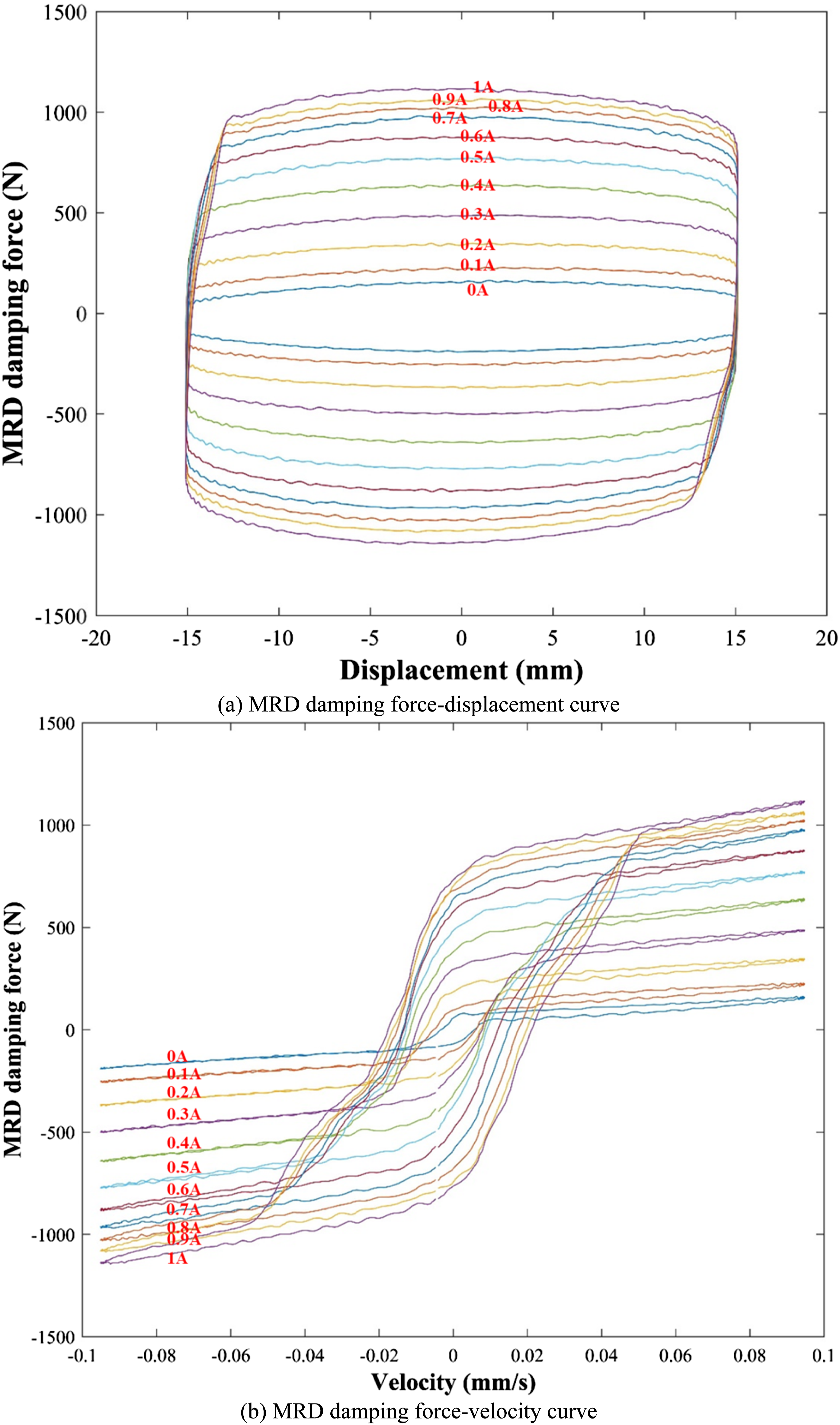
Parameter identification of Bouc-Wen model
Bouc-Wen model
The structure of the Bouc-Wen model of MRD
39
is shown in Figure 2, and its mathematical expression is as follows: Bouc-Wen model.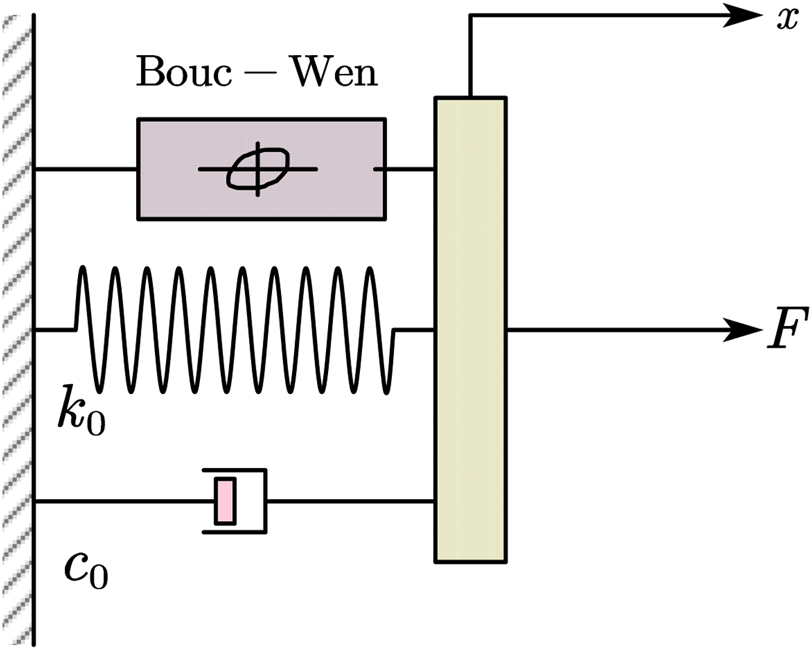


A designed Bouc-Wen model using MATLAB/Simulink, and a numerical simulation using the 4th order Runge Kutta method is performed here. The implementation process is depicted in Figure 3. Implementation of the Bouc-Wen model in MATLAB/Simulink.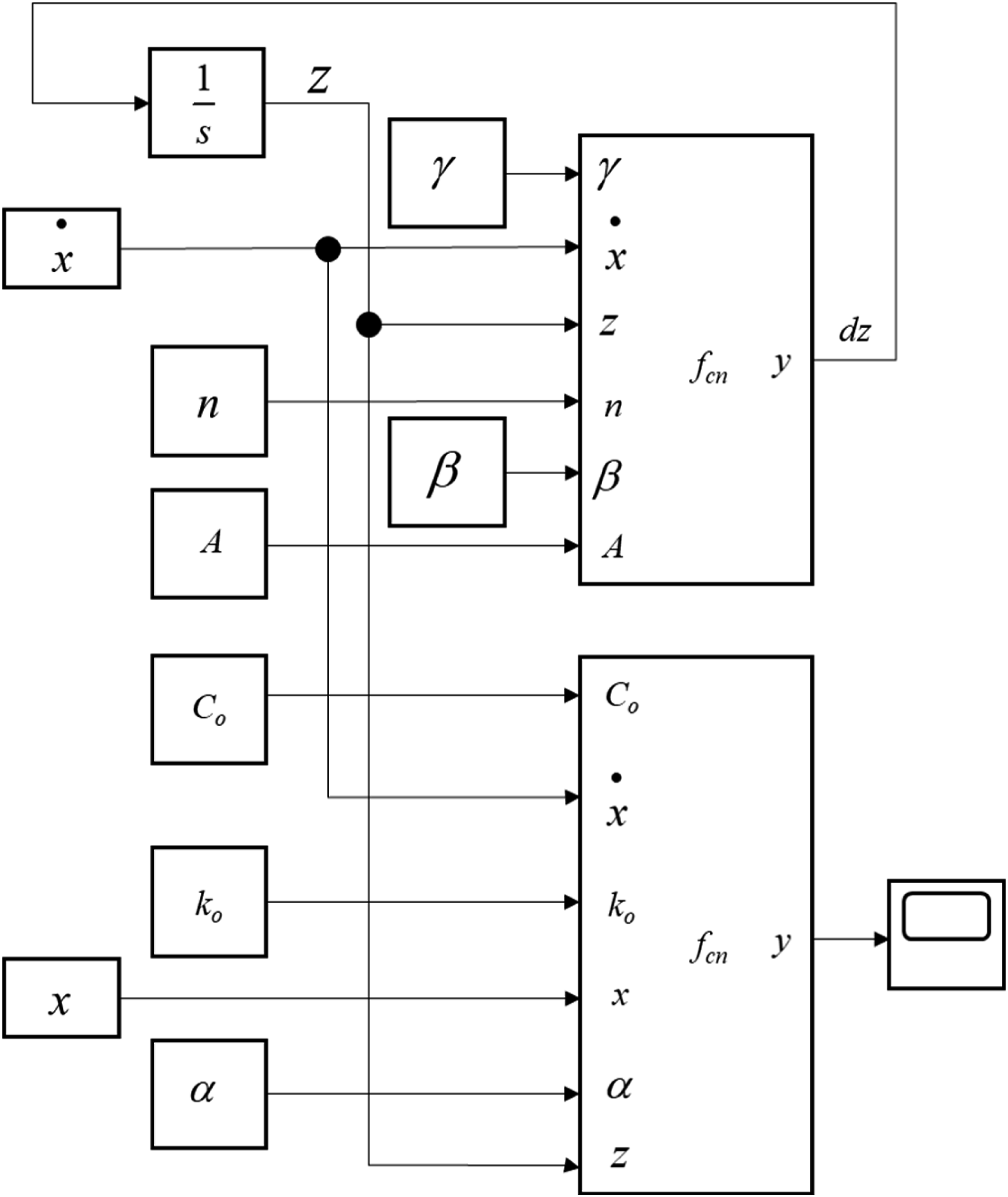
PSO algorithm
Natural systems, such as flocks of birds and schools of fish, often exhibit impressive, collision-free, synchronized interactions. These behaviors stem from the inherent reactions of everyone in the group, although their underlying reasons are quite complicated from a macro perspective. For instance, by maintaining an appropriate distance between each bird in the flock and its neighbors, the flock’s migration behavior can be simulated accurately. This distance depends on the bird’s size and behavior. On the other hand, when a school of fish swims freely, individuals maintain a large mutual distance, but in the presence of a predator, the school of fish will gather into a very close group.
A similar phenomenon also exists in physical systems, exemplified by particle aggregation due to Brownian motion or fluid shear force. Additionally, human beings exhibit homogenous behavior characteristics, especially in forming social organization hierarchies and beliefs. However, unlike physical systems, people can hold the same idea or viewpoint without disagreement. These simplified aggregation behaviors in natural, physical, and human social systems facilitate more in-depth experimental and simulation studies, thereby laying a foundation for developing swarm intelligence. Despite differences in the material structures of these systems, they have common properties with the following five basic swarm intelligence principles: 1. Distance: the ability to perform space and time calculations. 2. Quality: the ability to respond to environmental quality factors. 3. Diverse reactions: the ability to make various reactions. 4. Stability: maintaining stable behavior under slight environmental changes. 5. Adaptability: the ability to change behavior under the decision of external factors.
Furthermore, sharing social information between individuals within the system provides evolutionary advantages. Based on the aforementioned studies, Kennedy and Eberhan officially published an article titled ‘Particle Swarm Optimization' in 1995 at the IEEE International Neural Network Academic Conference, marking the birth of the PSO algorithm. Since then, this algorithm has been extensively used, promoted, and generalized in.40–46
The PSO algorithm starts by initializing a group of particles without volume and mass, with each particle representing a potential solution to the optimization problem. Subsequently, a pre-defined fitness function is employed to determine the quality of these particles. In general, all particles move within the problem’s search space, and the speed variable limits the particles’ direction and distance. Usually, the particle seeks the current optimal position in each generation, where each particle follows the individual and neighbor optimal position. The PSO algorithm is a new intelligent optimization algorithm that originates from the simple social simulation of birds and fish schools. Therefore, PSO algorithms can be used to simulate this interactive process, providing a new way to solve decision-making issues in complex environments.
The PSO algorithm is a random optimization technique based on swarm intelligence. This algorithm is inspired by social behavior based on bird flocking and employs a swarm of multiple particles, each with its own position and velocity. All particles share information obtained from other particles, and the interaction among the particles makes the search efficient. Each potential solution is also assigned to a randomized velocity, and potential solutions are called particles. These particles are then ‘flown' through hyperspace. Each particle keeps track of the coordinates associated with the best-achieved solution (fitness) in the hyperspace. This solution is referred to as ‘pbest'. All values of pbest for each of the particles are tracked simultaneously. By keeping track of the overall best value and its location, the globally optimized solution, gbest, can be obtained.47,48
The updating equations the of the velocities and positions of each particle are described as follows:
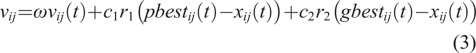

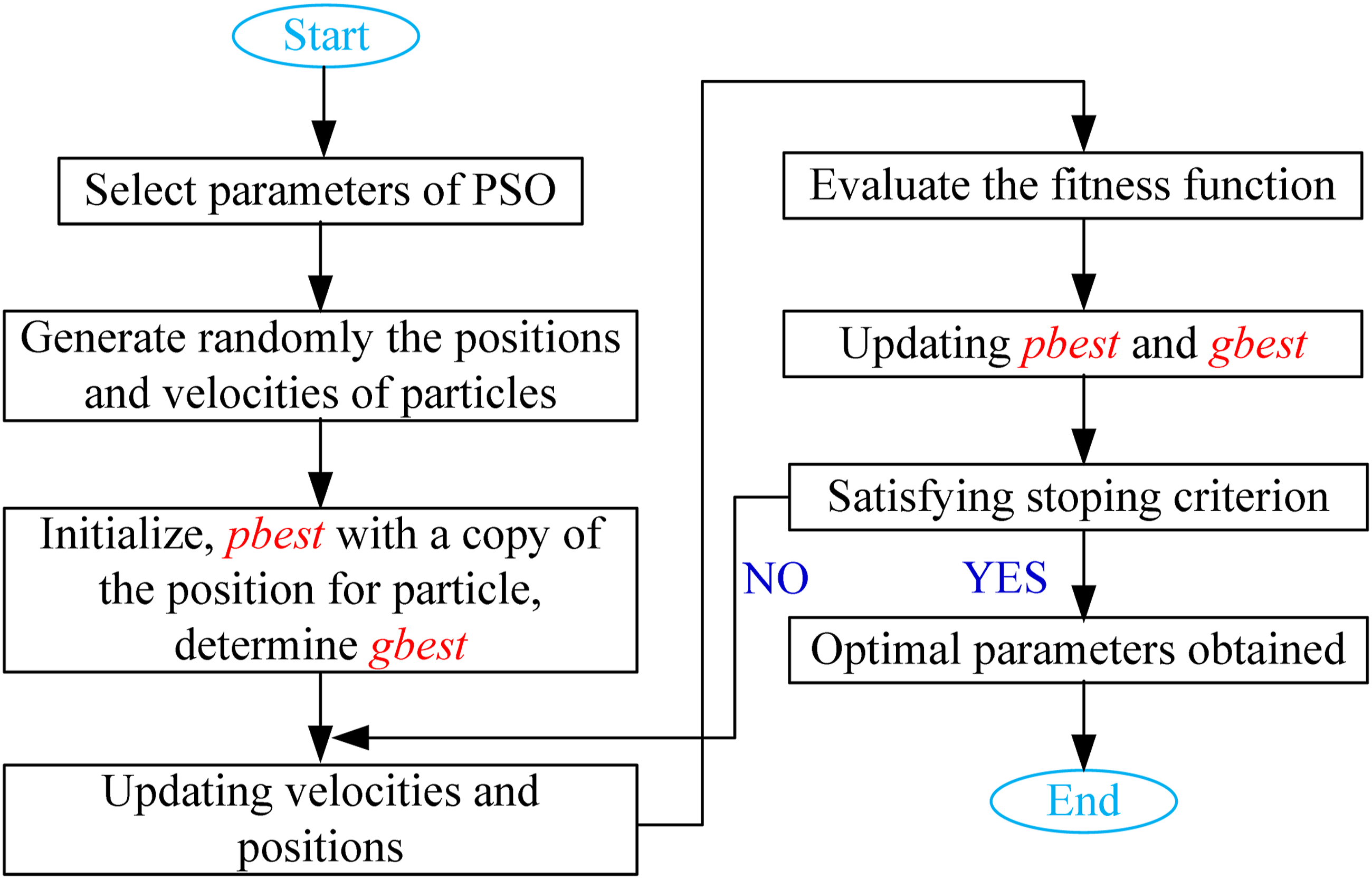
The inertia weight factor Basic structure of the PSO algorithm. Flowchart of the PSO algorithm.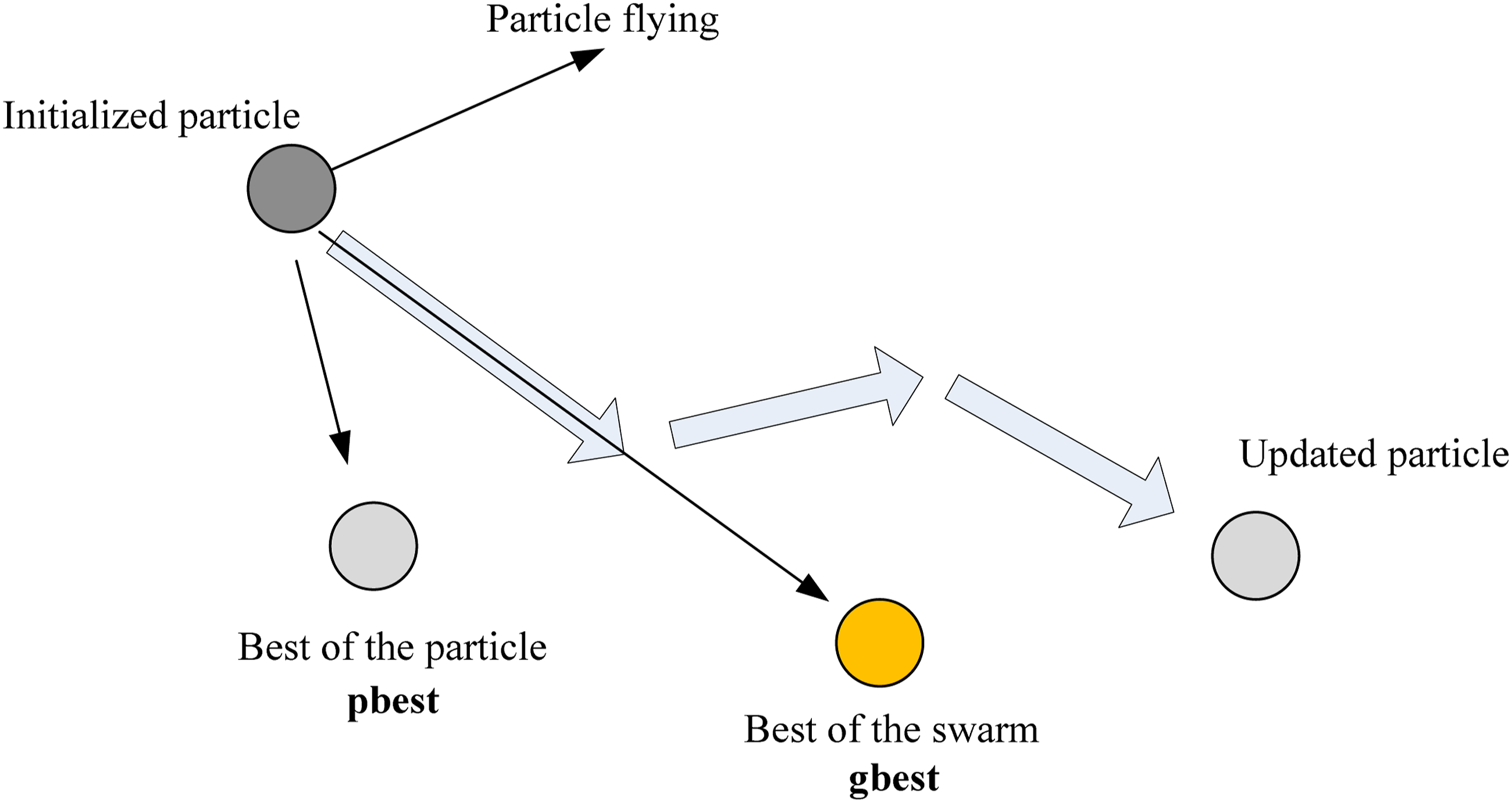
Parameter identification of Bouc-Wen model
There are a total of 8 unknown parameters in the Bouc-Wen model, including A, β, γ, α, c0, k0, n, and x0, which are difficult to be accurately identified using general iterative optimization algorithms.
Therefore, a proposed identification strategy for the Bouc-Wen model based on PSO is implemented in this paper. Before performing identification on the 8 unknown parameters of the MRD Bouc-Wen model, it is imperative to set a wide range of parameter values without any prior knowledge in addition to the data obtained through mechanical experiments.
The fitness function of the Bouc-Wen model is defined as follows:

Firstly, set the search range for the parameters A, β, γ, α, c0, k0, n, and x0 arbitrarily as [1, 1, 1, 1, 1, 1, 1, −1]∼[1 × 10⁴, 1 × 10², 1 × 10³, 1 × 10³, 50, 1 × 10², 3, 10].
Since there are 8 unknown parameters, the randomness of parameter identification results is high, and the identification has high requirements for the given search range. Hence, a necessary upper limit (UL) study of the 8 parameters should be performed, and a reasonable parameter search range can be determined sequentially.
Firstly, a search range study on parameter A is conducted, and the UL of A from 1 × 10⁴ to 2 × 10³ is adjusted. Then, the fitting effect of predicted MRD data is shown better than before. Reducing the UL does not change the fitting effect so much. Therefore, the reasonable UL of A is set to 2 × 10³. Similarly, the ULs for other parameters are optimized.
After varying the UL for β from 100 to 50 and 30, a reasonable UL of 30 was ultimately determined. After attempting from 1 × 10³ to 5 × 10² and 5 × 10³, the reasonable UL of γ was ultimately determined as 1 × 10³. The UL for α was adjusted from 1 × 10³ to 3 × 10², leading to a reasonable UL of 3 × 10². The UL attempt for c0 was changed from 50 to 5 × 10², 5 × 10³, 5 × 10⁴, and 5 × 10⁵, resulting in a reasonable UL of 5 × 10⁴. The UL attempt of k0 was changed from 100 to 1 × 10³, 1 × 10⁴, 5 × 10⁴, and 2 × 10³, with a reasonable UL of 1 × 10³. Finally, the UL for x0 was adjusted from 10 to 0.1 and 1, setting a reasonable UL of 1.
For parameter n, a phenomenon was found during the identification research process that except for the reasonable UL of 1A current, which needs to be set as 3, the other ULs for currents 0A∼0.9 A should be set as 2, a value proved more reasonable based on analysis.
In summary, the search range of A, β, γ, α, c0, k0, n, and x0 was determined as, [1, 1, 1, 1, 1, 1, 1, −1]∼[2 × 10³, 3 × 10², 1 × 10³, 3 × 10², 5 × 10⁴, 1 × 10³, 3, 1].
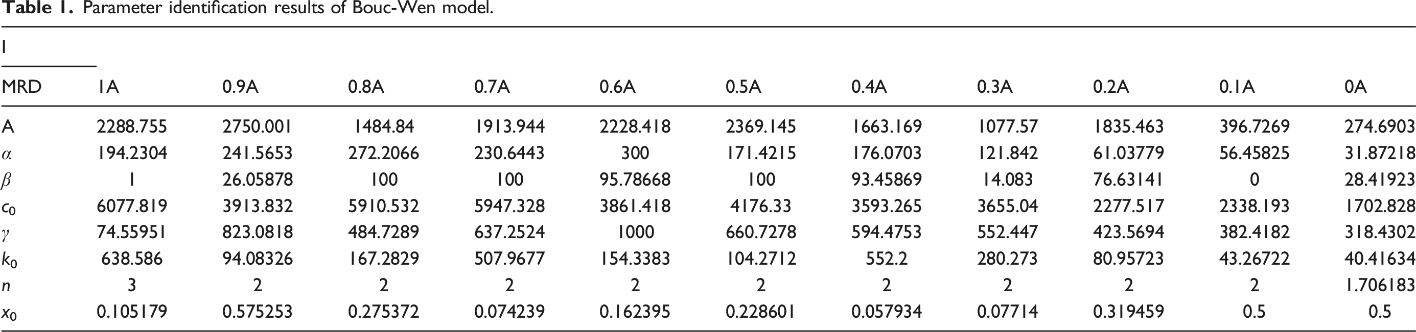
Parameter identification results of Bouc-Wen model.
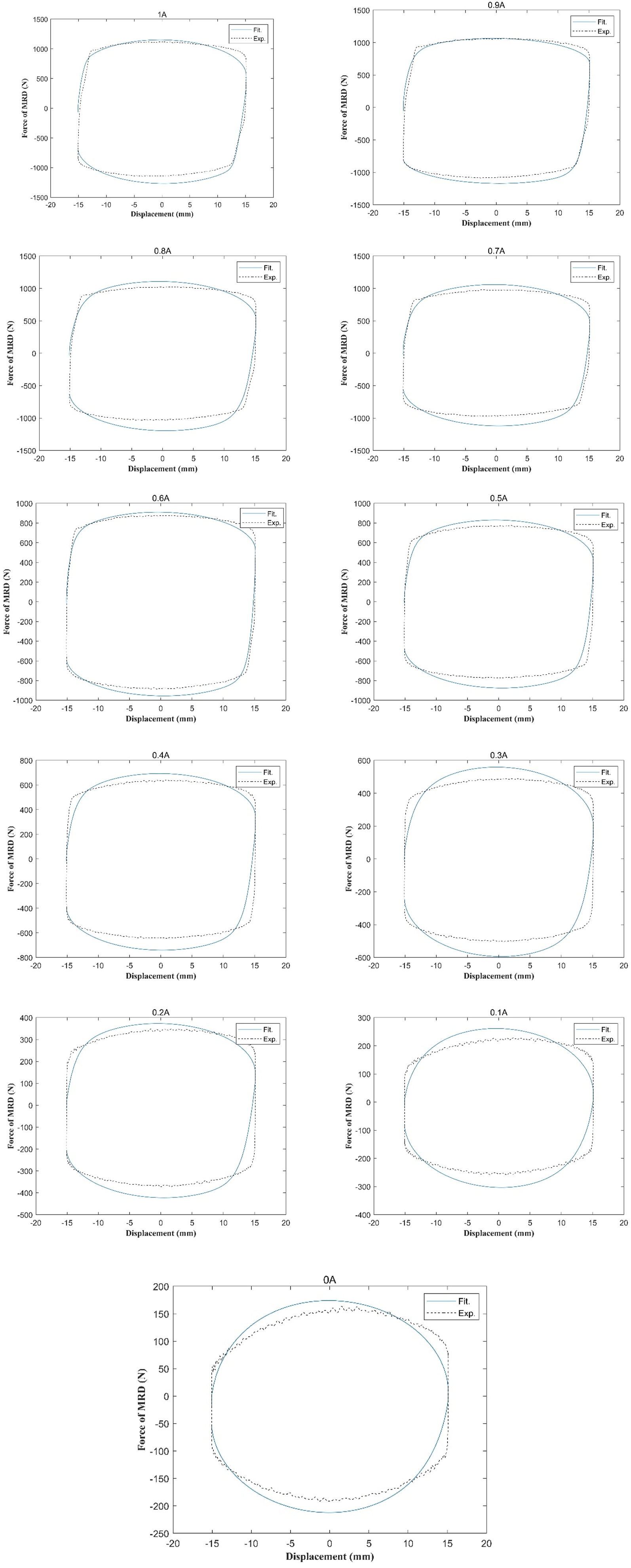
Comparison between MRD predicted output based on identified parameters and experimental data.
Next, the variation laws of the identified parameters of the MRD mechanical model under different currents are studied.
According to Figure 7, A oscillates with the increase of current. Within the range of 0∼0.5A, A demonstrates a basic increasing trend, while within the 0.5A to 0.8A range, A shows a decreasing trend. A increases between 0.8A and 0.9 A, while it decreases in the range of 0.9A to 1A. Within the range of 0A∼0.8A, as the current increases, α basically shows an upward trend, and in the range of 0.9A∼1A, it shows a downward trend. Variation pattern between identified parameters and current.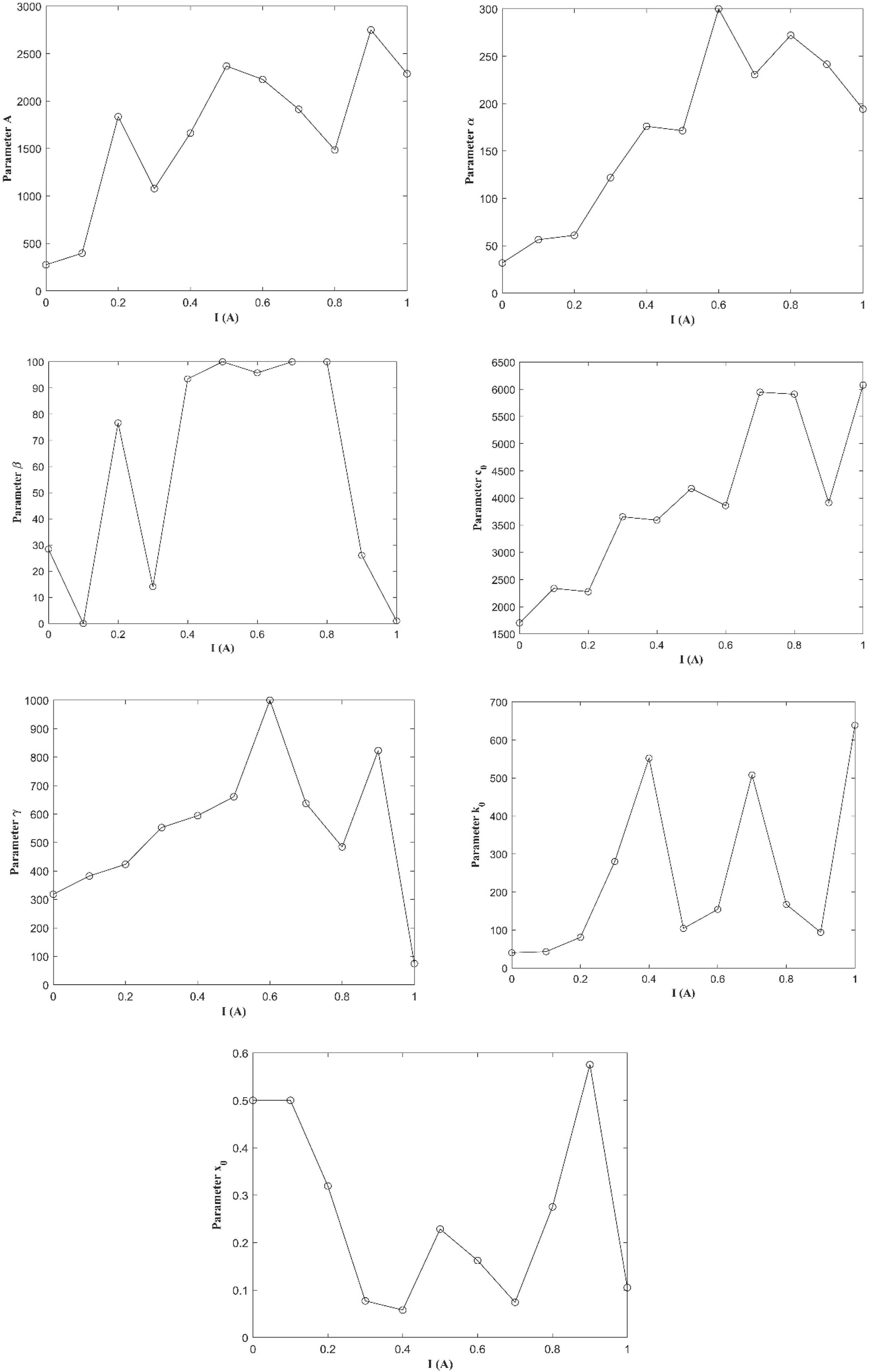
The changes in β are relatively random. Ranging from 0 to 0.4A, β shows oscillation variation. In the range of 0.4A∼0.8A, the change of β is very small, while in the range of 0.8A to 1A, β significantly decreases.
The change of c0 reveals a gradual upward trend. At 0.7A and 0.8A, it shows a significant increase. Then, it shows a significant decrease at 0.9A. Finally, 1A shows a significant rebound.
The change laws of γ are divided into two parts. Firstly, there is an increasing trend with the increase of current in the range of 0A∼0.6A. Then, there is an oscillatory trend when the current exceeds 0.6A. In the range of 0.6A∼0.8A, it shows a downward trend, followed by an upward trend in the range of 0.8A∼0.9A. Finally, it has a significant decrease at 1A.
The change of k0 appears serrated, exhibiting an increasing trend in the range of 0A∼0.4A, followed by a decrease at 0.5 A. Subsequently, there is an increase in the range of 0.5A∼0.7A, and it decreases in the range of 0.7A∼0.9A, while it has a rebound at 1A.
The change of x0 shows a W-shaped pattern. It shows a decrease trend in the range of 0A∼0.4A, while it has a rebound at 0.5A. Moreover, it decreases in the range of 0.5A∼0.7A while it increases in the range of 0.7A∼0.9A. Eventually, it has a significant decrease at 1A.
For parameter n, except for 1A and 0A, all others are 2.
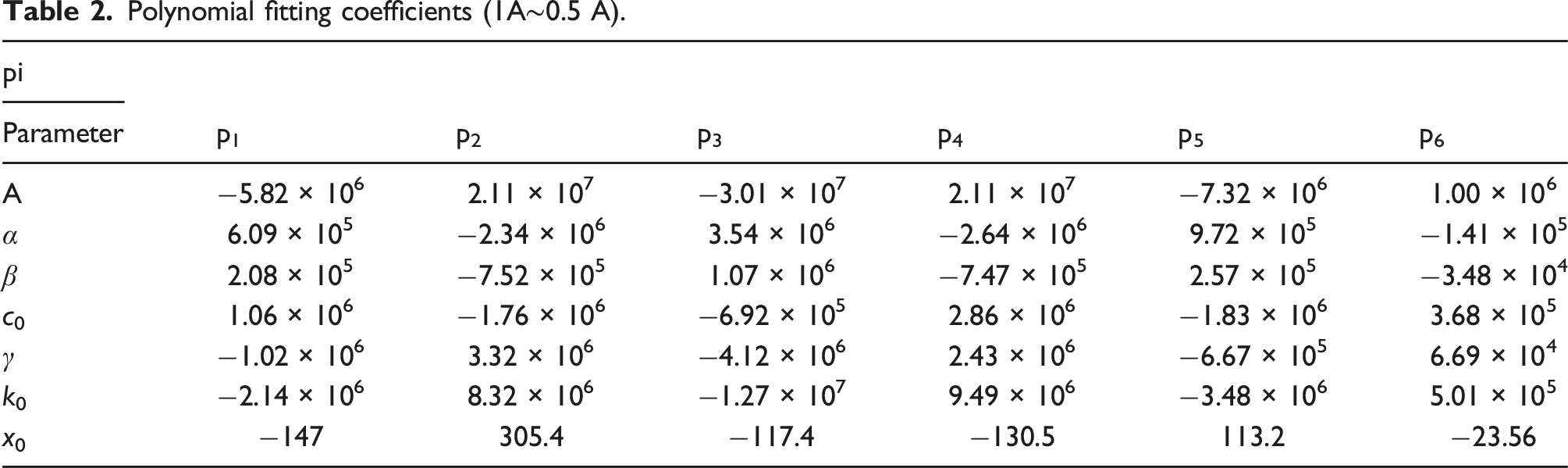
Polynomial fitting coefficients (1A∼0.5 A).
Polynomial fitting coefficients (0.5A∼0A).
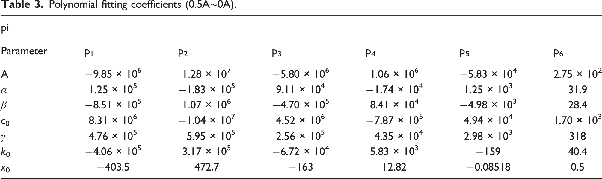
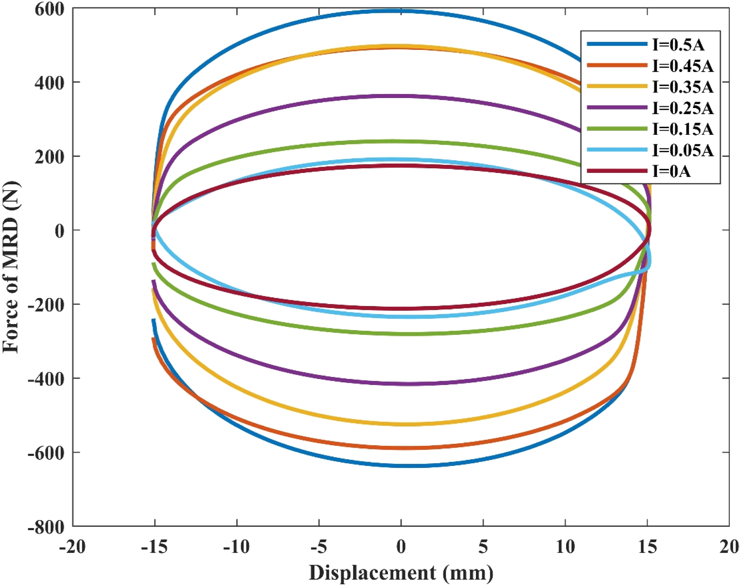
Based on the polynomial fitting of the above 7 unknown parameters with the current I, the MRD data of I = 0.55A, 0.65A, 0.75A, 0.85A, 0.95A, and 1.0A are predicted. Figure 8 shows the MRD output prediction of the current ranging from 1A to 0.5 A. Similarly, the MRD outputs of I = 0.5A, 0.45A, 0.35A, 0.25A, 0.15A, 0.05A, and 0A are also predicted, and Figure 9 presents the MRD output prediction for the current range of 0.5A to 0A. MRD output prediction of current 0.5A, 0.55A, 0.65A, 0.75A, 0.85A, 0.95A, and 1.0A. MRD output prediction of current 0.5A, 0.45A, 0.35A, 0.25A, 0.15A, 0.05A, and 0A.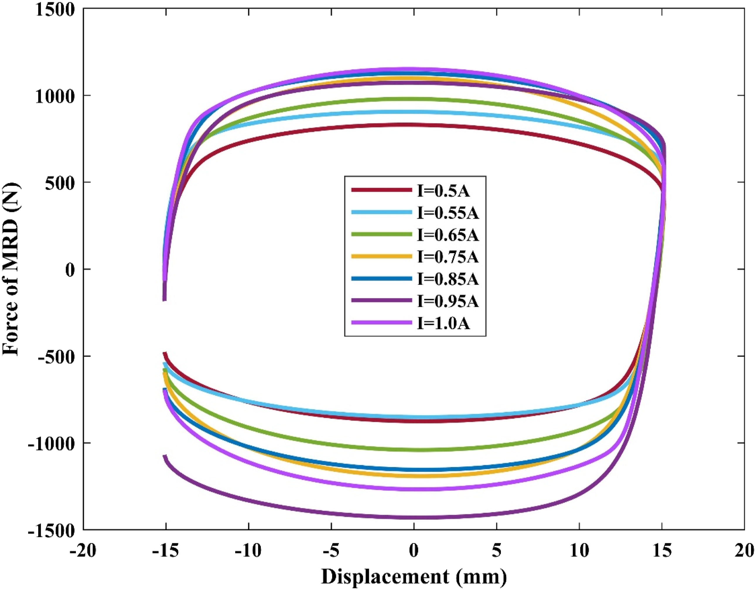
Application of MRD in semi-active control of power equipment
Vibration control models of power equipment
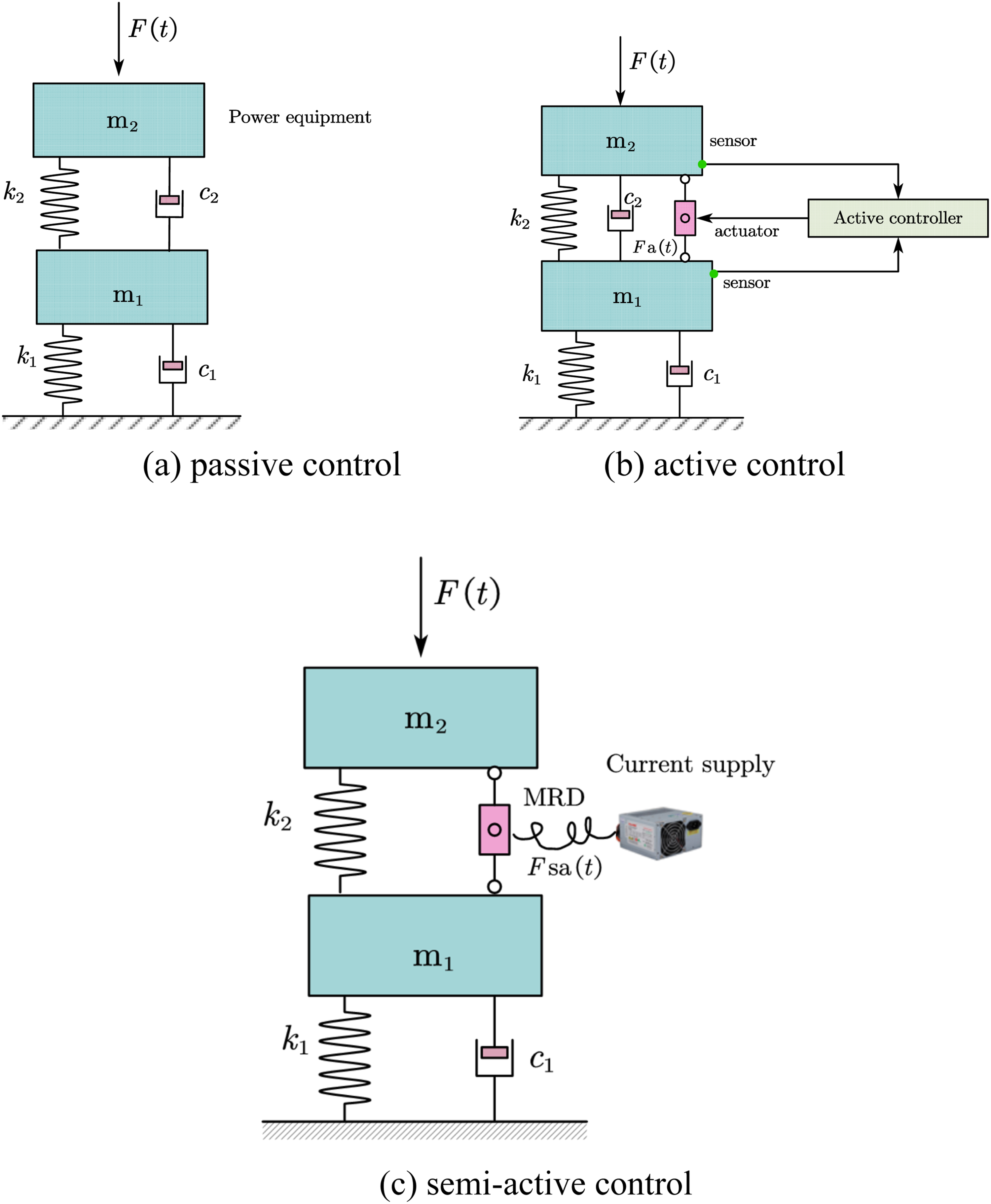
Figures 10 and 11 depict the passive, active, and semi-active control models of single-stage and two-stage vibration control for power equipment, respectively. In practical engineering, single-stage vibration control systems are more common. However, in scenarios where the power equipment is connected to the foundation and the mass ratio of the foundation to the equipment itself cannot be ignored, it is necessary to consider the participation of the foundation in vibration. Consequently, when the system requires to be designed as a two-stage system to overcome the shortcomings of a single-stage system,
49
research on a two-stage vibration control system should be conducted. Single-stage vibration control system for power equipment. Two-stage vibration control system for power equipment.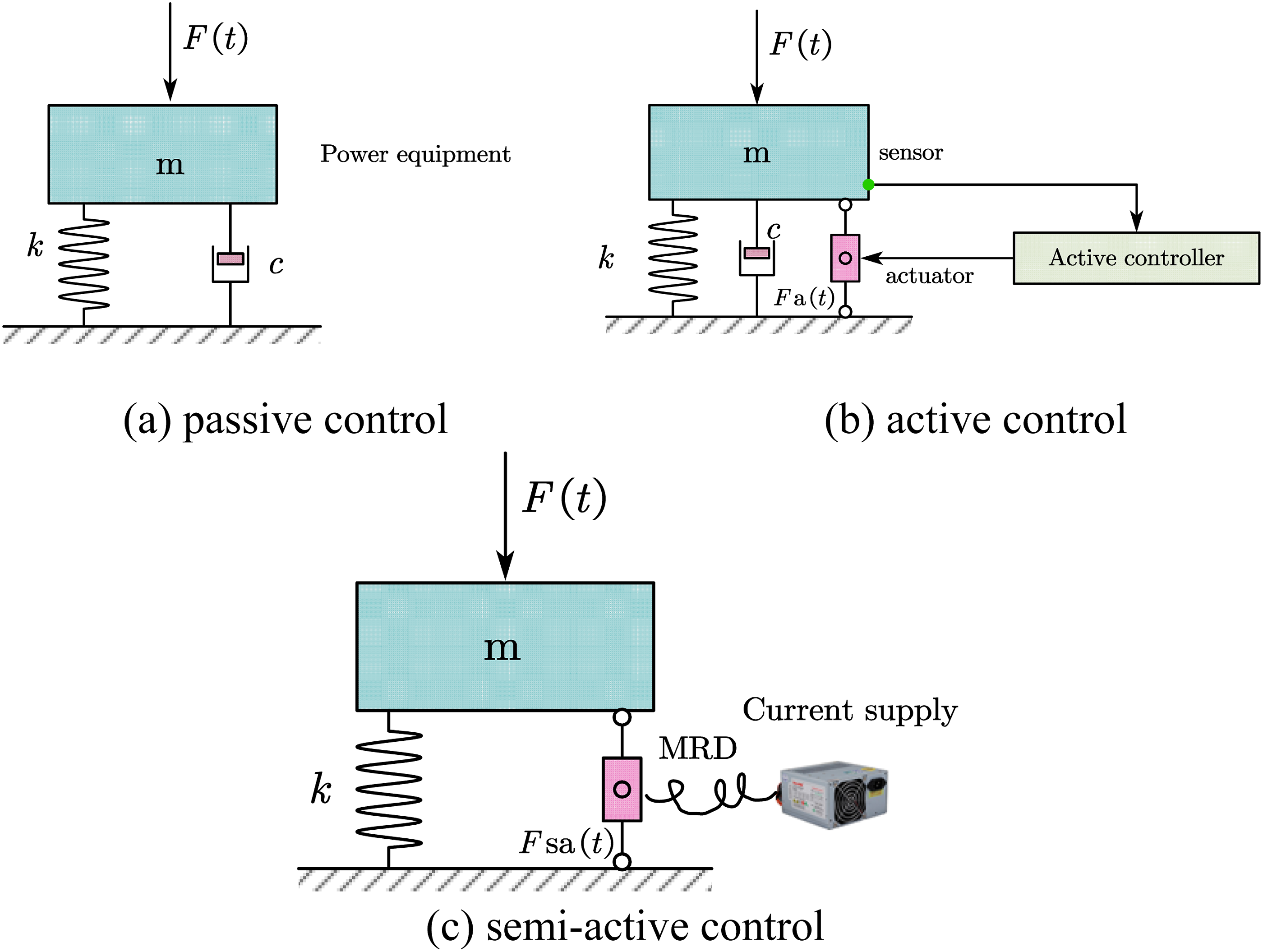
Theoretical derivations for semi-active control and compared PSO-LQR active control
In the single-stage vibration control system of the power equipment shown in Figure 10, assumes that the dynamic load generated by the equipment is 
For the two-stage vibration control system of the power equipment shown in Figure 11, m2 represents the mass of the power equipment, k2 and c2 denote the stiffness and damping of the isolation system, respectively, and m1, k1, and c1 indicate the mass, stiffness, and damping of the foundation or support structure, respectively. The load form is the same as that of a single-stage system. At this point, the displacement, velocity, and acceleration of equipment vibration are, respectively, 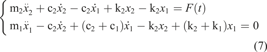
For the convenience of performing out active and semi-active control, the dynamic equation of the single-stage vibration control system is firstly transformed into the form of a state-space equation by setting the state variables 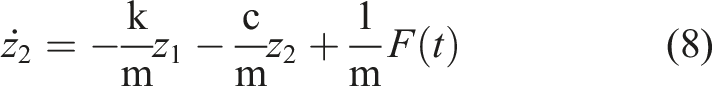
Change the above equation to state-space form as follows: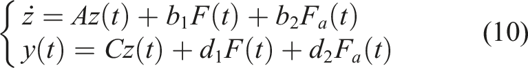
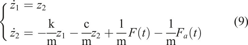
If it is a semi-active control system, equation (6) becomes: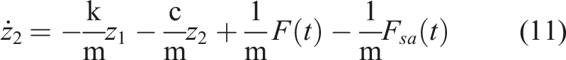
Let 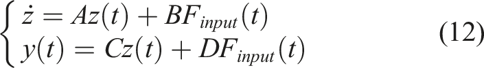
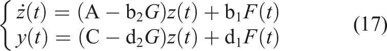
For a two-stage vibration control system, if it is an active control system, equation (7) can be transformed into the following form of the state-space equation by setting the state variables 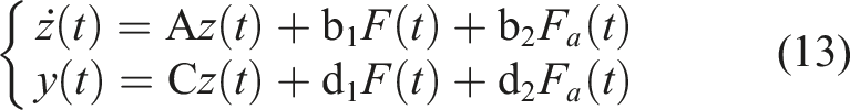
If it is a semi-active control system, equation (7) becomes the following form: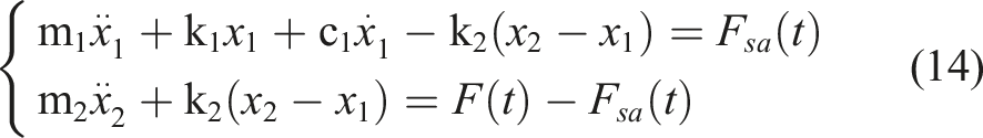
By setting the state variables 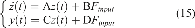
For both single-stage and two-stage vibration control systems, the LQR active control algorithm is employed for active control. For LQR active control, there are the following indicators: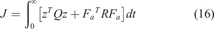
Based on the optimal feedback gain The LQR active control for power equipment.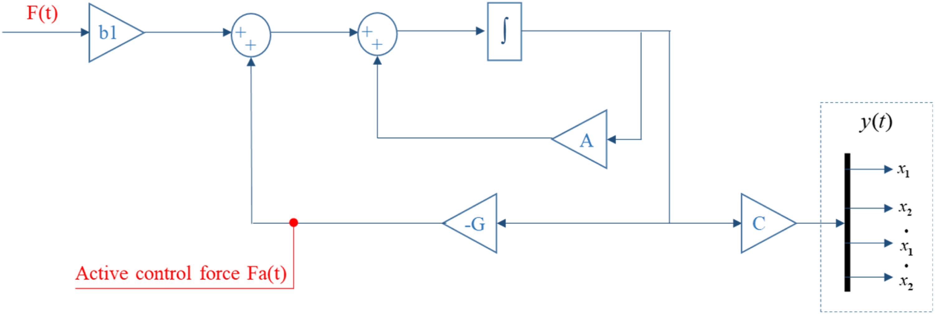
In the optimal control design of LQR, the selection of Q and R weight matrices significantly impacts control effectiveness and control force. The manner in which these matrices are established rationally and directly influences the optimal control outcome. Therefore, this study will establish a PSO-LQR active control strategy based on the PSO algorithm, as shown in Figure 13. Schematic diagram of PSO-LQR active control for power equipment.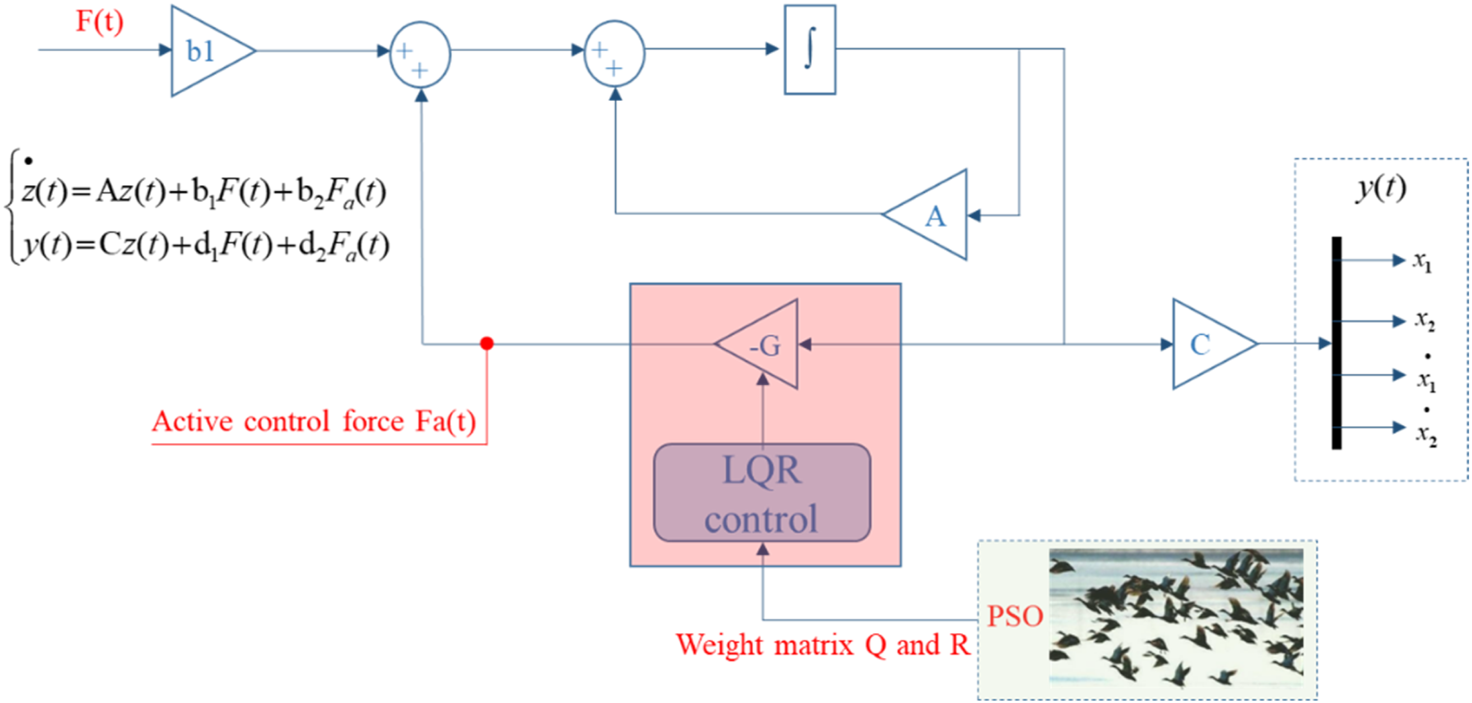
For the PSO-LQR active control shown in Figure 13, the fitness function Fitness is selected as
The parameter settings for a single-stage system are set as follows:
F(t) is a random vibration load with an amplitude of 5000 N, m = 500 kg, c = 10 N·s, and k = 1×10⁵ N/m.
The parameter settings for a two-stage system are set as follows:
Vibration load F(t) has the same form as the single-stage system, and m1 = 97,500 kg, k1 = 1.23×10⁹ N/m, c1 = 3.64×10⁶ N·s, m2 = 1958 kg, k2 = 7.72×10⁴ N/m, and c2 = 3.69×10³ N·s.
For the single-stage LQR active control, the search range for parameters q1, q2, and R is set as [1 × 10⁻⁴, 1 × 10⁻⁴, 1 × 10⁻⁴]∼[1 × 10⁴, 1 × 10⁴, 1]. For the two-stage LQR active control, the parameter search range for q1, q2, q3, q4, and R is set as [1 × 10⁻⁴, 1 × 10⁻⁴, 1 × 10⁻⁴, 1 × 10⁻⁴, 1 × 10⁻⁴]∼[1 × 10⁴, 1 × 10⁴, 1 × 10⁴, 1 × 10⁴, 1].
After calculation, the PSO optimization solution for q1, q2, and R of the single-stage LQR active control is [7.95 × 10³, 8.85 × 10³, 1 × 10⁻⁴], and the PSO optimization solution for q1, q2, q3, q4, and R of the two-stage LQR active control is [9.58 × 10³, 4.45 × 10³, 7.82 × 10³, 4.45 × 10³, 1 × 10⁻⁴].
Proposed semi-active control strategy
MRD can regulate the output damping force by adjusting the input current I. The most common semi-active control strategy utilizing MRD is switch control. In this study, on-off balance control is used for the single-stage systems, and on-off skyhook control is used for the two-stage systems.
50
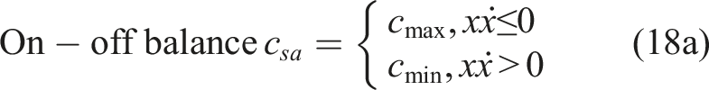
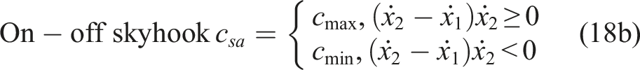
Where The proposed semi-active variable damping control strategies.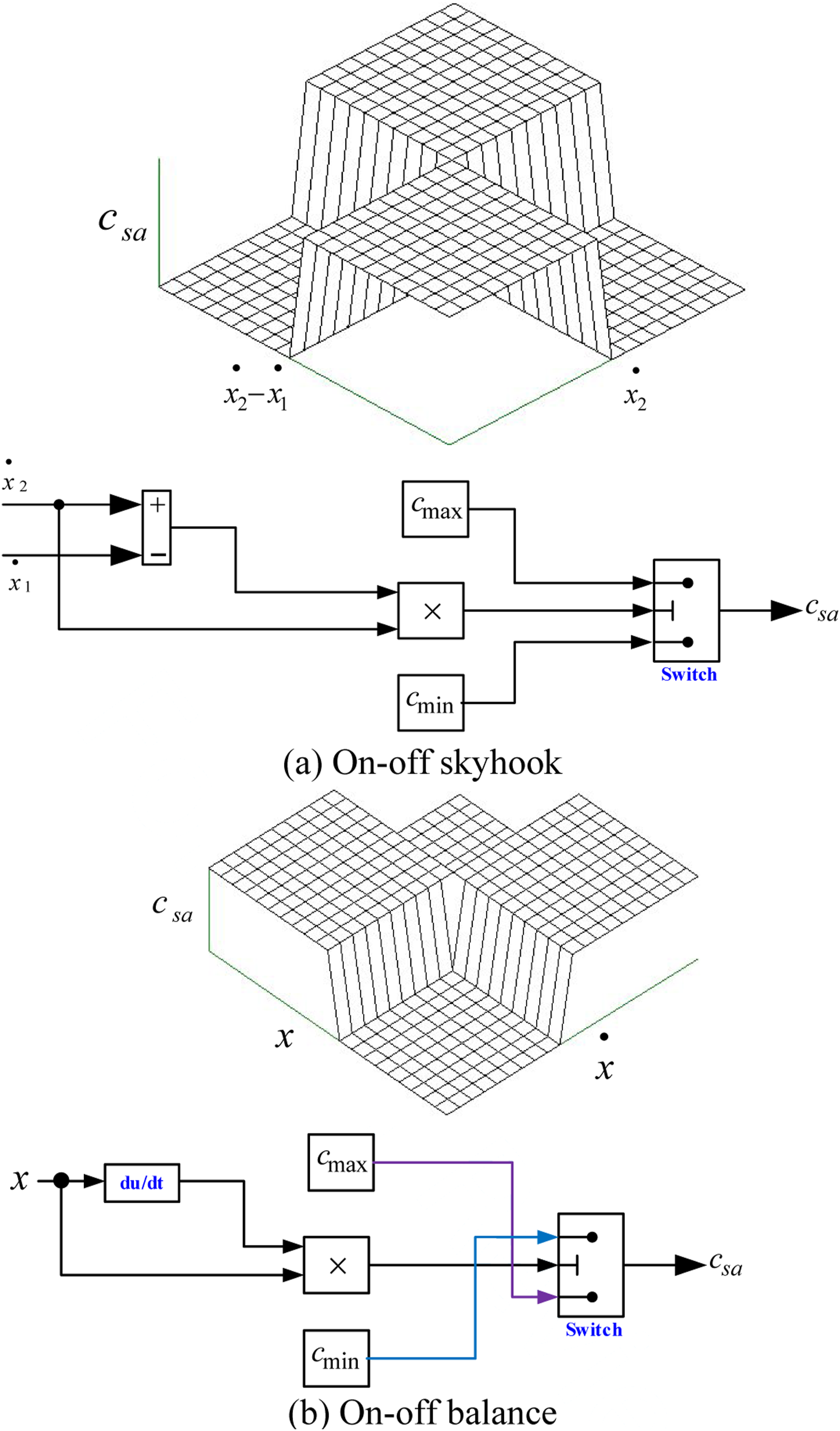
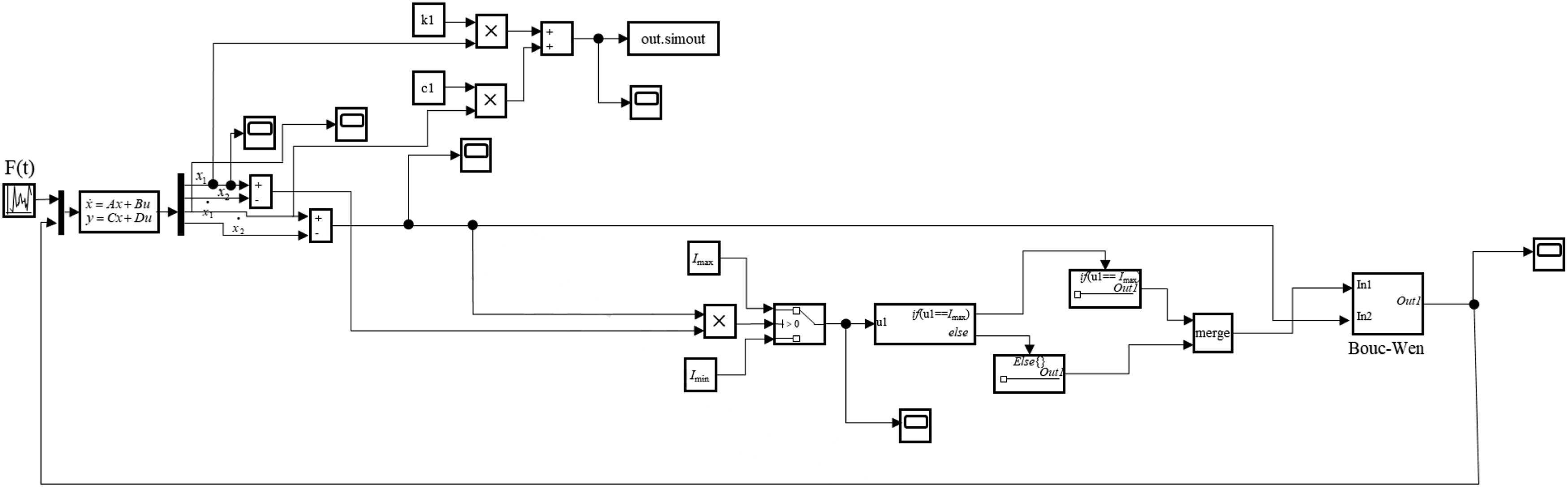
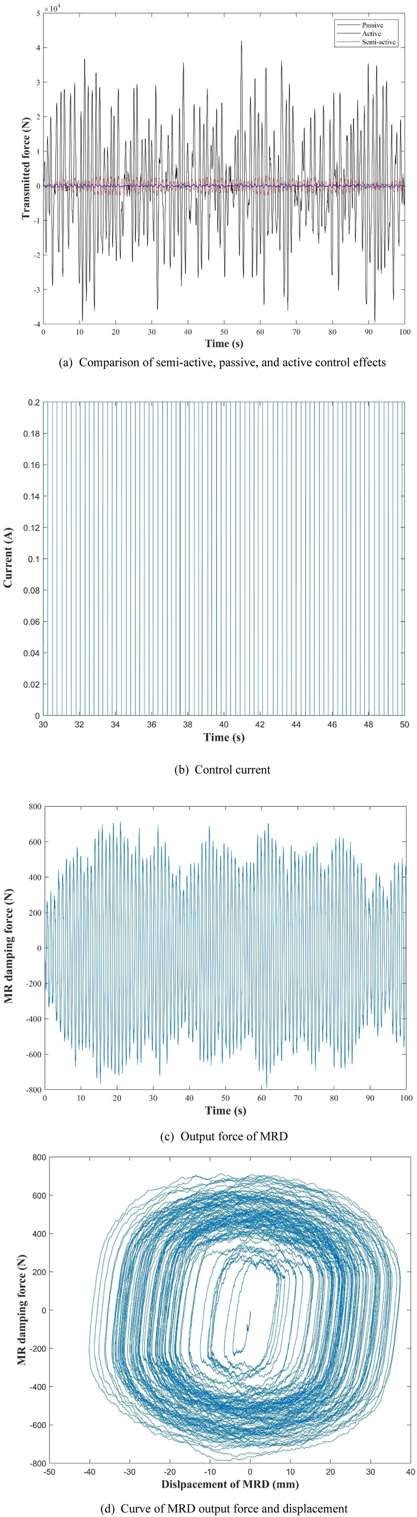
Figures 15 and 16 show the single-stage and two-stage MRD semi-active control calculation diagrams using Simulink, respectively. Figures 17 and 18, respectively, illustrate the semi-active control effects of single-stage and two-stage MRD semi-active control, alongside passive and PSO-LQR active control, offer a comparative analysis. At the same time, the control current and the relationship curves between output force and displacement of MRD are presented. Simulink calculation block diagram for MRD semi-active control (single-stage). Simulink calculation block diagram for MRD semi-active control (two-stage). Control response of single-stage system. Control response of two-stage system.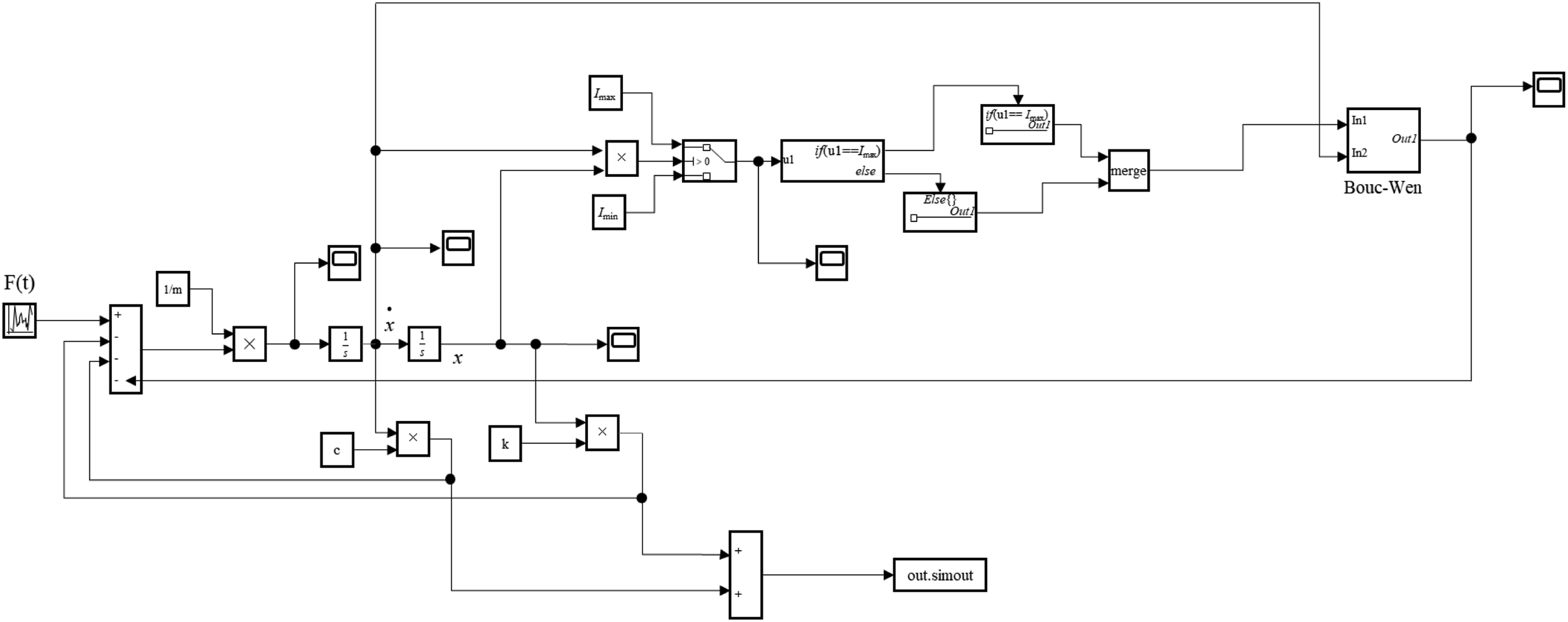
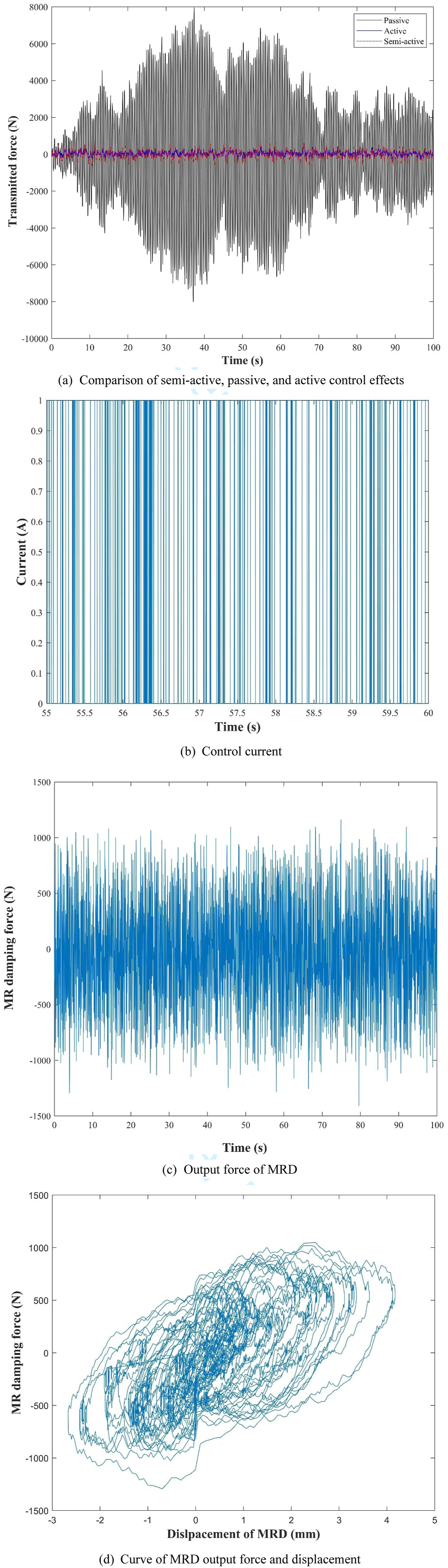
As shown in Figure 17(a), the active and semi-active control effects of a single-stage system are significantly better than passive control, and the semi-active control is slightly inferior to active control. Figure 17(b) shows the control current of the single-stage semi-active system (only results from 55s to 60s are displayed). Figure 17(c) shows the semi-active control output force of MRD, which indicates that the MRD output force is relatively uniform and reasonable. Figure 17(d) shows the relationship curve between MRD motion displacement and output force, which indicates that it is a hysteresis shape with an oblique ellipse.
According to Figure 18(a), the semi-active control effect of the two-stage system is significantly better than passive control, and it is also slightly inferior to active control, and this law is consistent with that of the single-stage system. Figure 18(b) shows the control current of a single-stage semi-active system (only results from 30s to 50s are displayed). Figure 18(c) shows the semi-active control output force of MRD, which is relatively uniform and reasonable. Figure 18(d) shows the relationship curve between MRD motion displacement and output force, which shows a slightly inclined and relatively plump elliptical hysteresis.
Conclusions
Under the condition of having no prior knowledge other than experimental data, the PSO technique was used to identify 8 unknown parameters of the Bouc-Wen model for the MRD. This study simultaneously investigated the variation law of these parameters with current and the identification results are verified. Then, single-stage and two-stage vibration control models were developed for power equipment, and the identified Bouc-Wen model was applied to establish a semi-active control system based on MRD in the vibration control of power equipment. Subsequently, a calculation program was established in MATLAB/Simulink and a comparative study was also conducted using passive and active control. The active control was a PSO-based LQR control, and the parameters of the active controller were optimized based on the PSO technique. The results showed that the adopted semi-active control can significantly reduce the transmitted force from the power equipment to the foundation and effectively decrease the disturbance of the power equipment to the environment. The effect of semi-active control was significantly better than passive control while slightly inferior to active control. This study has important guiding significance for the vibration control application of MRD in industrial engineering, laying a foundation for more in-depth research on semi-active control in modern industrial engineering.
Footnotes
Acknowledgments
The authors wish to acknowledge the Key Youth Fund of SINOMACH (Grant no. QNJJ-ZD-2022-04), research and application of key technologies for micro-nano environmental vibration control of chinese major science and technology infrastructures. The authors also wish to acknowledge Prof. Lei Xie of Chongqing University and Prof. Anzhong Zhao of SINOMACH.
Declaration of conflicting interests
The author(s) declared no potential conflicts of interest with respect to the research, authorship, and/or publication of this article.
Funding
The author(s) disclosed receipt of the following financial support for the research, authorship, and/or publication of this article: This work was supported by the the Key Youth Fund of SINOMACH; QNJJ-ZD-2022-04.