Fuel poverty and rebound effect in South Korea: An estimation for home appliances using the modified regression model

Abstract

Since the occurrence of oil shocks in the 1970s, a number of countries have introduced fuel poverty programs. However, rebound effects could be problematic even in these programs. In particular, there are two controversies surrounding rebound effects: the magnitude of rebound effects and the influence of income on these effects. This study attempts to resolve these issues by empirically estimating the rebound effects of individual home appliances for low-income households. Thereafter, it compares the rebound effects for low-income families with those for all-income families. Analyses results suggest that the magnitude of rebound effects highly depends on individual home appliances, and that these effects are usually larger for low-income households. Thus, the differences in rebound effects between all-income and low-income households also depend on individual appliances. Therefore, policy-makers should meticulously consider the rebound effects of individual home appliances when planning energy efficiency programs.

Keywords

Fuel poverty rebound effect backfire effect direct estimation concavity super conservation

Introduction: Efficiency improvement and fuel poverty

Despite the important role of energy efficiency as a climate change mitigation strategy, there have been arguments between economists and policy-makers on whether market or government intervention is necessary to induce energy efficiency. Since the occurrence of oil shocks in the 1970s, most countries have introduced various energy conservation policies to reduce the consumption of fossil fuel and electricity. Typical examples of these policies are efficiency improvement programs such as national minimum energy efficiency threshold, efficiency labeling of products, energy service companies, and Energy Efficiency Resource Standards.¹

During this period, scholars argued that although advanced and financially viable technologies to improve efficiency were available in the market, these were not actively utilized by consumers.² This phenomenon was well known as “market failure” of energy efficiency improvement, and several reasons have been put forward for the occurrence of this phenomenon.³ For example, consumers could not purchase efficient home appliances owing to incomplete information. In addition, transaction cost, adverse selection, principal–agent relationship, and hidden cost are other reasons for market failure in energy efficiency.

However, economists, in particular neo-liberalists, have opposed government intervention regarding efficiency improvement. They believe in the voluntary allocation of resources by the market, not the government. In other words, only the price solely determines the utilization of resources and energy.⁴ For example, if the price of electricity increases, consumers will purchase highly efficient appliances to reduce their expenditure. By contrast, if the price decreases, they tend to consume more electricity with inefficient appliances. In particular, some researchers argued that government intervention is nonessential for energy efficiency improvement because governments nearly do not intervene with regard to the efficiency of other resources such as steel, wood, and cement.⁵

In addition, economists have argued that “government failure” is more severe than market failure. Namely, although the market does not function properly, the cost provoked by governments’ intervention could be larger than the loss from the malfunction of market. In other words, the inefficiency of governments is worse than the inefficiency of market.⁶ Under these circumstances, fuel poverty programs could serve as a solution to overcome these controversies. This is because utilizing minimum energy is regarded as a basic human right. In other words, fuel poverty programs are beyond economic issues because these are closely related to welfare issues. In fact, some advanced countries such as the UK, the US, and Germany have attempted to provide minimum energy to the poor for decent living.⁷ This clarifies the undoubted role of the government in overcoming fuel poverty.

Despite this undebatable role of the government in the field of fuel poverty programs, the “rebound effect” is still inevitable. The rebound effect initially originated from Jevon’s Paradox, which was suggested in 1865 and well conceptualized by Khazzoom in 1987.⁸ In short, the “rebound effect” is defined as the difference between the expected energy savings and the actual energy savings owing to the actual price decrease after efficiency improvement. Although fuel poverty programs are certainly provided by the government, energy efficiency improvement resulting from this program may have a rebound effect as well. Moreover, the relationship between the rebound effect and income level is also debatable. In other words, while some researchers have insisted that rebound effects are larger for low-income households, others have found totally different empirical results.⁹

Therefore, as some fuel poverty programs aim to improve energy efficiency among low-income households, estimating the rebound effects of these programs is necessary. This study attempts to identify which groups have larger rebound effects between all-income households and low-income households. In the same context, Galvin¹⁰ suggested that a subject-oriented policy is important in the field of energy. In other words, policy-makers should target “behavers,” not behaviors for desirable energy programs. This study estimates the rebound effects for home appliances in South Korea, which is one of the fast-growing countries.

The remainder of this study is structured as follows. The next section reviews the background, definition, and typical programs of fuel poverty. The “Theoretical background: Rebound effects and low-income households” section explains the basic theory and controversies surrounding the rebound effects. The “Rebound effects of low-income households in South Korea” section presents an estimation of rebound effects for low-income households and compares the results with those for all-income households. Finally, the “Conclusion and policy implications” section concludes the study and suggests policy implications.

A brief review of fuel poverty programs

History, definition, and status of fuel poverty

The interest in fuel poverty has increased since the outbreak of oil shocks in the 1970s. So far, the concept of fuel poverty has been actively adopted in a few advanced countries such as the UK, the US, Ireland, and New Zealand.¹¹ Governments in these countries have attempted to provide basic energy service to the poor suffering from a sudden rise in fuel price. The UK government describes a household to be in the state of fuel poverty if the household spends over 10% of the annual income for heating.¹² In the case of the US, the government adopted a similar concept, “energy burden,” for which the criterion was 10.9%.¹³

Fuel poverty occurs due to several reasons. First, the deficiency of income is a basic factor. Second, the poor are unable to purchase enough fuel owing to the priority of other expenditure. Third, a rise in fuel price could be a burden for the poor. According to previous studies, if energy price increases 1%, then the proportion of households in fuel poverty augments 0.05%.¹⁴ Fourth, inefficiency of housing and appliances induces extravagant consumption of energy. Thus, fuel poverty affects human health negatively and provokes chronic diseases such as asthma and pneumonia.¹⁵

Today, fuel poverty is still a severe social problem.¹⁶ In the US, official data from the Department of Health and Human Services show that low-income families consume less energy than non-low-income families. Namely, while non-low-income families consume 52.8 mmBtu and spend US$389 per year, low-income families consume only 41.6 mmBtu and spend US$314 for natural gas and electricity.¹⁷ Similarly, fuel poverty is a serious concern in the EU. The average percentage of the population that is deprived of electricity is 6.8% for all EU countries, while the percentage in Slovenia is 15.5%. Even in the UK, the percentage is 10.6%, which is larger than the average of all EU countries.¹⁸

Fuel poverty programs in selected countries

Earlier, fuel poverty was regarded as an important issue only in a few countries. Consequently, only the UK, the US, and Ireland had introduced social programs for fuel poverty. However, after the occurrence of the most recent oil shock that lasted from 2004 to 2008, most countries launched fuel poverty programs.¹⁹

The UK is a pioneer in adopting fuel poverty programs. The country has very systematic programs in place to reduce the proportion of people living in fuel poverty.²⁰ For example, based on the “Warm Homes and Energy Conservation Act,” which was enacted in 2000, the government established a fuel poverty strategy in 2001 and has published progress report annually.²¹ Nevertheless, while the government aimed to eradicate fuel poverty by 2016, the goal was not achieved owing to economic crisis and rise in energy prices.

In this country, a typical program for fuel poverty is the “Warm Front.” This program provides funds to low-income households living in the private housing sector for house insulation, efficient heating equipment, and so on. Ultimately, the government expects the households to reduce cost and improve thermal comfort.²² Other fuel poverty programs in the UK are Decent Home Standards, Warm Zones, Community Energy Efficiency Fund, Winter Fuel payment, and “Know your rights” campaign.²³

Another leading country to introduce fuel poverty programs is the US. Based on “the Energy Conservation and Production Act,” which was established in 1976, the Department of Energy has been responsible for implementing fuel poverty programs.²⁴ In this country, two remarkable fuel poverty programs are the Weatherization Assistance Program and the Low Income Home Energy Assistance Program. The Weatherization Assistance Program aims to reduce energy cost by improving efficiency, similar to the UK’s Warm Front Program. This program is often regarded as a “low-hanging fruit” with potential to solve structural inefficiency, increase energy independence, and mitigate climate change problems.²⁵ Therefore, more than 100 thousand households receive funds annually under this program. Additional grant is provided to households having any handicapped, elder, or younger persons.²⁶ The Low Income Home Energy Assistance Program was introduced by the “Omnibus Budget Reconciliation Act” that was enacted in 1981.²⁷ The Department of Health and Human Services is in charge of implementing this program. This program aims to satisfy the immediate energy needs of the poor in fuel poverty. Furthermore, the budget for this program could be also used for the Weatherization Assistance Program.²⁸

South Korea is a latecomer with respect to fuel poverty programs. The government of South Korea declared the goal of “Energy Poverty Zero” in 2007. In addition, it founded the Korea Energy Foundation, the specialized organization for fuel poverty programs. In 2009, the government also announced that it will establish a basic human right to consume minimum energy and improve the delivery system to solve the problem of energy poverty in “the Five Years Plan for Green Growth.” Specifically, the government provides the poor with emergent energy supply, house insulation, discounted tariffs, obligatory energy supply in winter, replacement of obsolete appliances with new ones, and safety inspection. Among all fuel poverty programs, the most important one is the Korean Weatherization Assistance Program, the efficiency improvement program for house insulation.²⁹

As observed in the cases of the three countries, efficiency improvement is the most prominent measure for the eradication of fuel poverty. In other words, most policy-makers have focused on house insulation programs. Nevertheless, some researchers have paid attention to efficiency improvement programs of home appliances. For example, Langevin et al.³⁰ indicate that although low-income households in the US have a strong willingness to purchase high efficient appliances with the Energy Star mark, they cannot afford to do so in the present. They provide evidence for this preference and behavior by interviewing 50 residents living in fuel poverty. Yang and Zhao³¹ conducted a survey of 526 Chinese respondents regarding the purchase of efficient equipment. The survey result suggested that income is indirectly related to individuals’ purchase behavior for efficient appliances. They conclude that governments should provide subsidies to poor families living in fuel poverty.

In fact, most countries have adopted efficiency improvement programs of home appliances to eradicate fuel poverty. For example, the Brazilian government has replaced old inefficient refrigerators with new efficient ones based on the “Energy Efficiency Law” since 2002. The government also expanded the budget and scale of the program in 2005. At that time, 11 million refrigerators among the total 50 million refrigerators were considered obsolete, using chlorofluorocarbon, one of the strongest greenhouse gases. By replacing the old inefficient refrigerators with new efficient ones, the government could receive carbon reduction credits from the EU emission trading scheme.³² The Chinese government introduced financial subsidy programs for the purchase of efficient appliances in 2009 and expanded the programs to include eight categories of efficient equipment in 2012. In the case of South Korea, the government has replaced obsolete appliances with efficient ones such as lighting equipment, refrigerators, and boilers.³³

Therefore, this study attempts to focus on the efficiency improvement of not houses, which serve as the target of the weatherization program, but of home appliances, for which rebound effects are expected to vary widely. Before conducting the main analysis, the basic theory of rebound effects will be explained in the next section. In addition, controversies surrounding the magnitude and influence of income with regard to rebound effects will be reviewed.

Theoretical background: Rebound effects and low-income households

Definition of rebound effect

Rebound effect is a relatively well-known and articulately defined concept. Since Khazzoom conceptualized the negative results of efficiency improvement as rebound effects in 1987, most scholars have followed his definition.³⁴ After Brookes proved that rebound effects could appear in the economy widely in 1990, the theory of rebound effect was developed into the “Khazzoom Brookes Postulate.” Currently, it is believed that theoretical consensus on rebound effect has been achieved.

Basically, rebound effect is related with the economic response to engineering measures for energy efficiency improvement.³⁵ For example, when a government provides subsidy to replace inefficient light bulbs with efficient LED lamps, energy saving can be expected based on the difference of efficiency before and after improvement. In other words, if all conditions are same without efficiency improvement, the so-called ceteris paribus condition, the amount of electricity consumption could be reduced. However, consumers perceive a decline in the energy service price after efficiency improvement. In other words, they are able to receive lighting service at a lower cost owing to efficiency improvement. Consequently, this economic mechanism tends to provoke unexpected overconsumption of energy. To sum up, rebound effect is defined as the part of expected energy savings taken-back after efficiency improvement as shown in the following simple equation

Rebound effect = \frac{expected savings - actual savings}{expected savings}

(1)

There are three widely accepted categories of rebound effects: direct, indirect, and economy wide rebound effects.³⁶ The “direct rebound effect” is linked to consumers’ behavior with respect to the same appliances. Owing to a decline in energy service price, consumers tend to utilize the appliances more. The “indirect rebound effect” is related to the utilization of other appliances. The decrease in energy service price owing to energy efficiency improvement could encourage consumers to utilize other appliances as well that require more energy. The “economy wide rebound effect” is the broadest effect. The fall of energy service price induced by efficiency improvement could affect the entire market and manufacturing system. If consumers utilize other appliances, then the change of demand for the other appliances could affect prices of labors, materials, and energy.³⁷ However, this study solely focuses on the “direct rebound effect.” This is because the targets for efficiency improvement programs are appliances or equipment, and not sectors or the entire economy. In other words, other rebound effects may have weak policy implications.

Controversies surrounding the rebound effect

As observed in the “Definition of rebound effect” subsection, while the concept of rebound effect has a long history and the definition is simple, there are several controversies surrounding this effect. Among them, the most critical issue is the magnitude of rebound effect. In fact, this controversy is not new. Earlier, Greening et al.³⁸ conducted meta-analysis to summarize the size of rebound effects. They reviewed 75 estimates from previous studies on rebound effects. They concluded that all estimates were less than 100% and most of them were moderate. Thereafter, a number of researchers have cited and accepted this conclusion. For example, Grepperud and Rasmussen³⁹ estimated rebound effects in Norway using a general equilibrium assessment. They found that the estimates were weak or close to zero except for the manufacturing sectors. Decisively, Nadel argued that rebound effects tend to be modest. Specifically, after reviewing previous studies, he summarized that direct rebound effects are less than 10% and indirect rebound effects are around 11%.⁴⁰ Therefore, he suggested that policy-makers need not be concerned about these effects because even the combined effect would come up to just about 21%.

In contrast, others have revealed deep concerns regarding rebound effects. For example, Saunders⁴¹ insisted that rebound effects could be larger than 100% theoretically and this phenomenon might occur in the real world in selected cases. Recently, Galvin⁴² identified extremely high rebound effects in newer EU countries. The estimates vary from 100 to 550%. In conclusion, the magnitude of rebound effects varies depending on individual countries, sectors, and appliances. Therefore, policy-makers should meticulously consider empirical studies on rebound effects when considering energy efficiency programs.

Another interesting controversy regarding the rebound effect is the influence of income. A number of researchers agree that rebound effects depend on income. This consensus originated from the initial study by Khazzoom.⁴³ Thereafter, most researchers have accepted this hypothesis. In fact, several empirical results have proven that income is a critical determinant of the magnitude of rebound effects. Therefore, rebound effects are assumed to be larger in the situation of low income because these effects are induced by unsaturated demand. Specifically, income could influence rebound effects at two levels: international and domestic levels.

First, income is a critical factor to decide the international difference of rebound effects. While rebound effects are lower in advanced countries, these effects are higher in undeveloped and developing countries because there is enormous unmet demand for energy services in these countries. By conducting meta-analysis, Chakravarty et al.⁴⁴ demonstrated that empirical estimates were larger in developing countries than in developed countries.

Second, income could domestically determine the magnitude of rebound effects. Compared with high-income households, low-income households suffer from poverty. Therefore, they have tremendous potential demand for energy services. In Germany, Madlener and Hauertmann⁴⁵ showed that while rebound effects were 12% for house owners, they were 40% for tenants. In the same group of tenants, while the rebound effects for high-income families were 31%, those were 49% for low-income families. In Australia, Murray⁴⁶ reached a similar conclusion by analyzing official data of 6957 households. Based on the result, he suggested that policy-makers should target high-income households to reduce energy consumption and greenhouse gases emission because low-income families have higher rebound effects.

In contrast, other researchers hold a totally different opinion. Saunders⁴⁷ insisted that rebound effects were substantially different from income effects. After scrutinizing time-series data for the US from 1987 to 2002, he showed that while income has increased and efficiency has been dramatically improved, energy consumption has augmented. In addition, the lowest-income households consumed more energy in 2002 than they did in 1987. In conclusion, he affirmed that rebound effects are independent from income effects.

In the midst of this controversy, Chitnis et al.⁴⁸ showed an interesting result using expenditure data of 6000 households in 2009. They estimated rebound effects for various categories of energy efficiency improvement in UK households. Their methodology was based on expenditure elasticity. They showed that rebound effects are modest (0–32%) for measures influencing energy consumption, larger (25–65%) for measures influencing vehicle fuel consumption, and very large (66–106%) for measures focusing on reduction of food waste. Moreover, they found that programs for low-income households had the largest rebound effects.

Thus, the same conclusion regarding the first controversy can be applied to this controversy as well, namely rebound effects for low-income households also depend on countries and individual appliances. Therefore, this study attempts to estimate rebound effects for low-income families in South Korea, focusing on three major home appliances: television, refrigerator, and washing machine.

Method of estimation

In order to measure the magnitude of rebound effects, appropriate estimation methods are essential. Chakravarty et al.⁴⁴ categorized 12 types of measures including direct relative measure, elasticity parameter measure, Cobb–Douglas technology function, and computable general equilibrium model. Thus, the magnitude of rebound effects varies depending on the type of measure.

However, it is widely perceived that quantification of rebound effects is awfully difficult.⁴⁹ A number of researchers have estimated rebound effects using the elasticity parameter measure, which is a relatively simple method. Nevertheless, the estimation of rebound effects for low-income households is more difficult because their dwelling condition is highly complicated and energy consumption data for this group are insufficient.

Given this situation, this study adopts “the modified regression model” to estimate rebound effects for low-income households. This method has two remarkable merits with regard to rebound effects. First, the model is able to estimate rebound effects for home appliances, while the most frequently utilized method, the elasticity measure, usually calculates rebound effects only at the sector level. Second, this model has an advantage of separating rebound effects from income effects. As seen in the “Controversies surrounding the rebound effect” subsection, income could influence rebound effects. Therefore, this model is considerably useful because it excludes income effects from rebound effects by including an income variable in the equation.

This method was initially conceived by Haas et al.⁵⁰ to estimate rebound effects of heating in Austria. The authors investigated the difference in the linear and nonlinear relationships between energy consumption and efficiency. Then, they concluded that the gap implies a rebound effect, and the difference was referred to as “concavity,” as seen in Figure 1

Rebound effect = \frac{Expected savings - Actual savings}{Expected savings} = \frac{E_{real 2} - E_{expected}}{E_{real 1} - E_{expected}}

(2)

Figure 1.

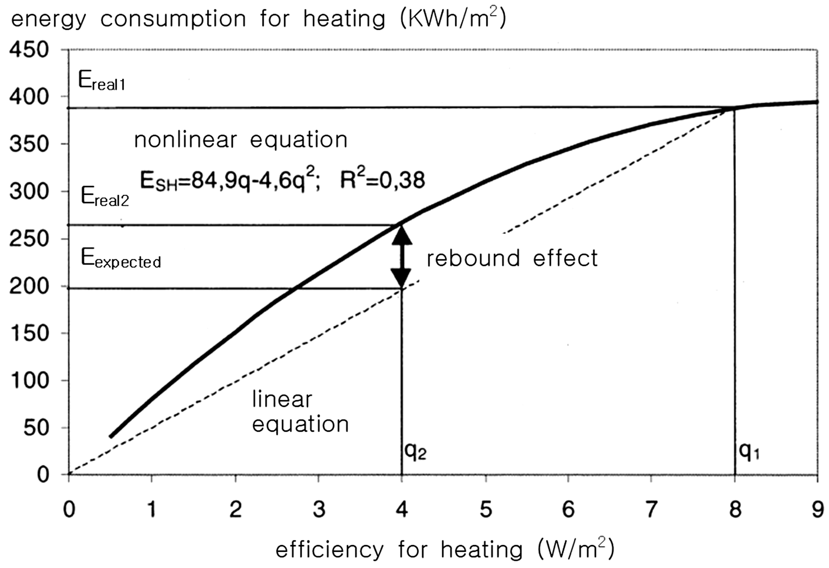
Rebound effect for the nonlinear relationship between energy consumption and efficiency. Source: Modified from Haas and Biermayr.⁵¹

E_real1: real energy consumption before efficiency improvement

E_real2: real energy consumption after efficiency improvement

E_expected: expected energy consumption after efficiency improvement

After an income variable was included in the regression model, this method was named as “the modified regression model.”⁵² As seen in equation (3), the modified regression model includes the polynomial equation of efficiency (q) and an income variable (I). This modification enables the model to separate rebound effects from the income effect. In fact, a number of studies show that there is interaction between income and rebound effects⁴⁷

Modified regression equation : E = aq + b q^{2} + c q^{3} + d q^{4} + e q^{5} + fI

(3)

E: energy consumption, I: income, q: efficiency, a, b, c, d, e, f: parameter

As Haas and Biermayr⁵¹ mentioned, the rebound effects in this model depend on a starting point. Thereafter, a standardized procedure of four steps was suggested.⁵³ In the first step, a nonlinear equation has to be decided for the relationship between energy consumption and efficiency. A stepwise method for multiple regression analysis was usually applied in previous studies to determine a polynomial equation. In the second step, the starting point should be determined. In general, the ninth grade is regarded as the low-efficient starting point.⁵⁴ In this analysis, actual efficiency data are divided into 10 grades, and the first grade means the highest efficiency while the 10th grade stands for the lowest efficiency. In the third step, target points for efficiency improvement should be specified. Usually, multi-targets are accepted from the first to the fourth grade because these grades are generally classified as high rank. Finally, in the fourth step, rebound effects can be estimated using the modified regression model.

It is necessary to identify three extraordinary cases related to rebound effect in the regression model. Figure 2(a) shows 100% rebound effect because there is no energy savings after efficiency improvement. In Figure 2(b), the rebound effect is greater than 100%, which is referred to as the “backfire effect” because efficiency improvement augments energy consumption. Lastly, Figure 2(c) is an extremely exceptional case because the rebound effects are below zero. It implies that there is “super conservation” after efficiency improvement. This paradoxical phenomenon was explained in the micro level by Galvin.⁴² The author exemplified that after replacing the old boiler with the efficient one, a consumer could reduce the energy service owing to the dearth of budget. In particular, this minus value of rebound effects could appear for the poor because they suffer from deficiency of income.

Figure 2.

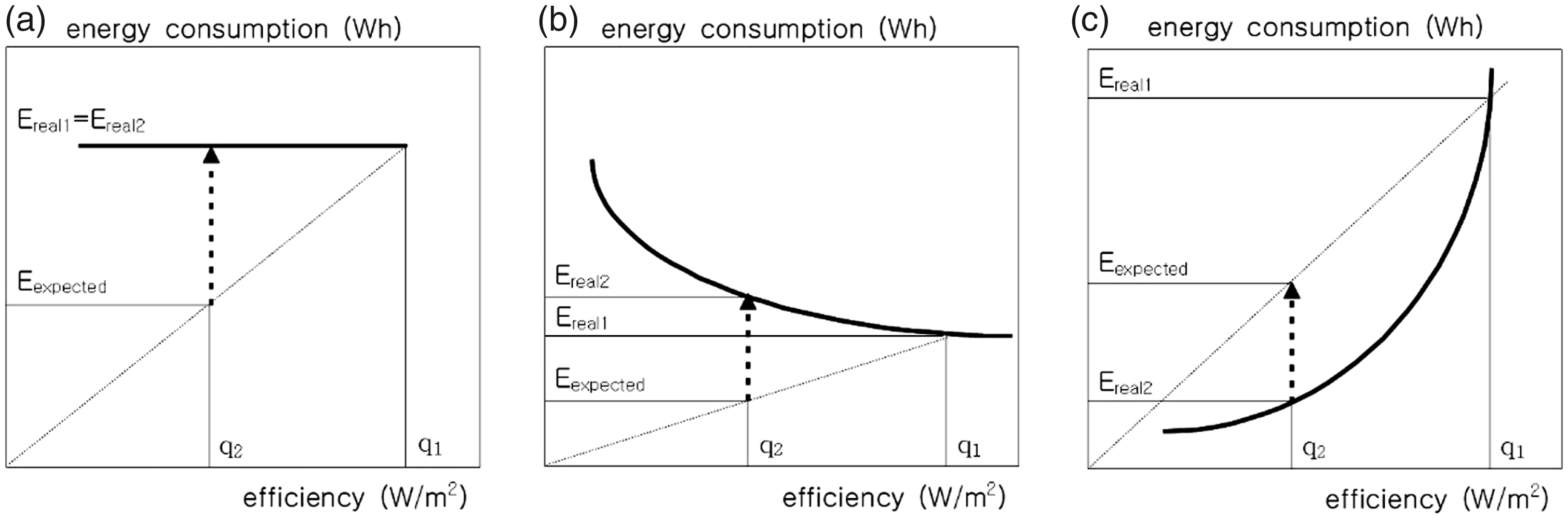
The three exceptional cases of rebound effects in the nonlinear relationship. Source: Jin.⁵² (a) (RE = 1). (b) (RE > 1). (c) (RE < 0).

Figure 3.

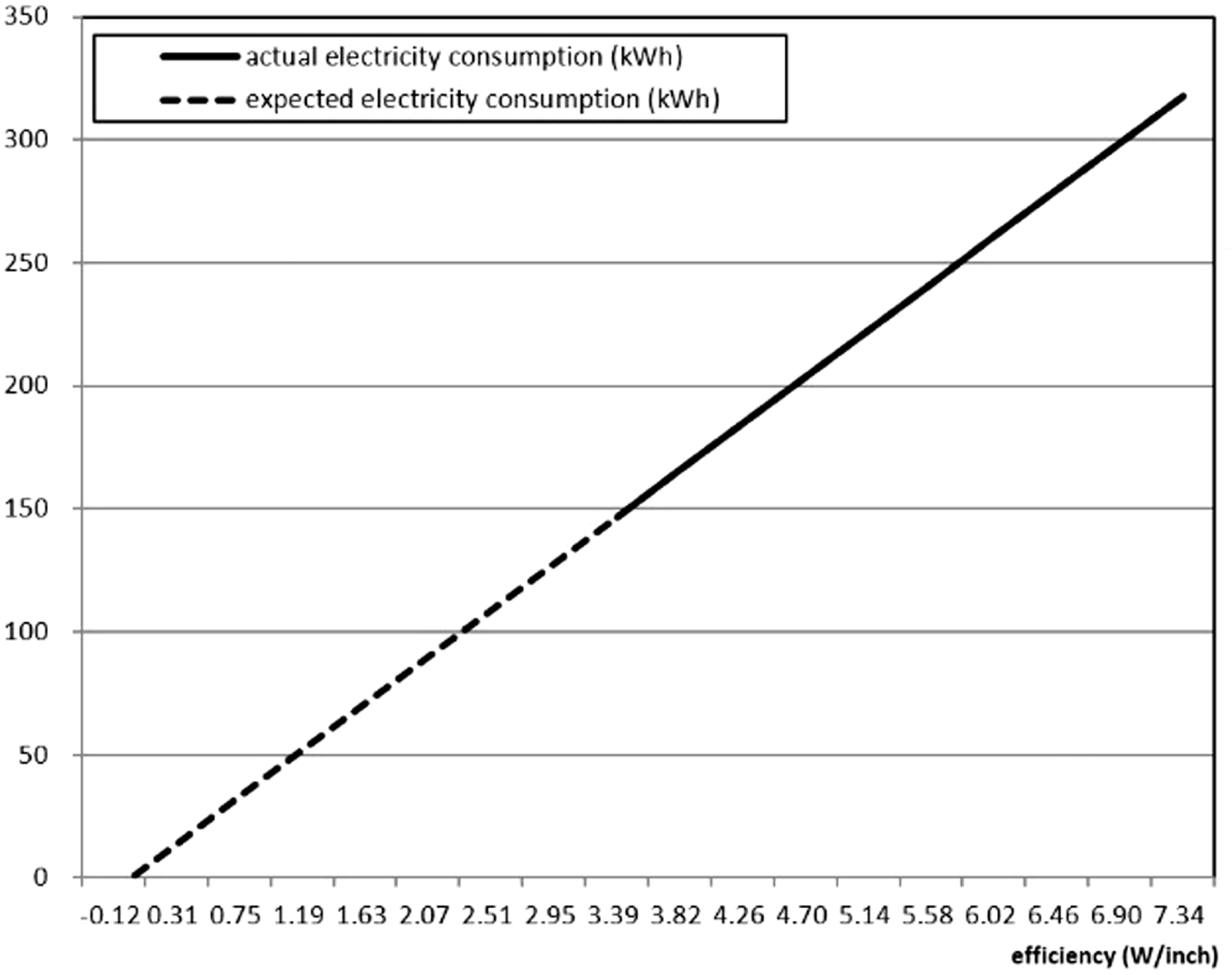
Linear relationship in televisions for all-income households. Source: Jin.⁵²

Figure 4.

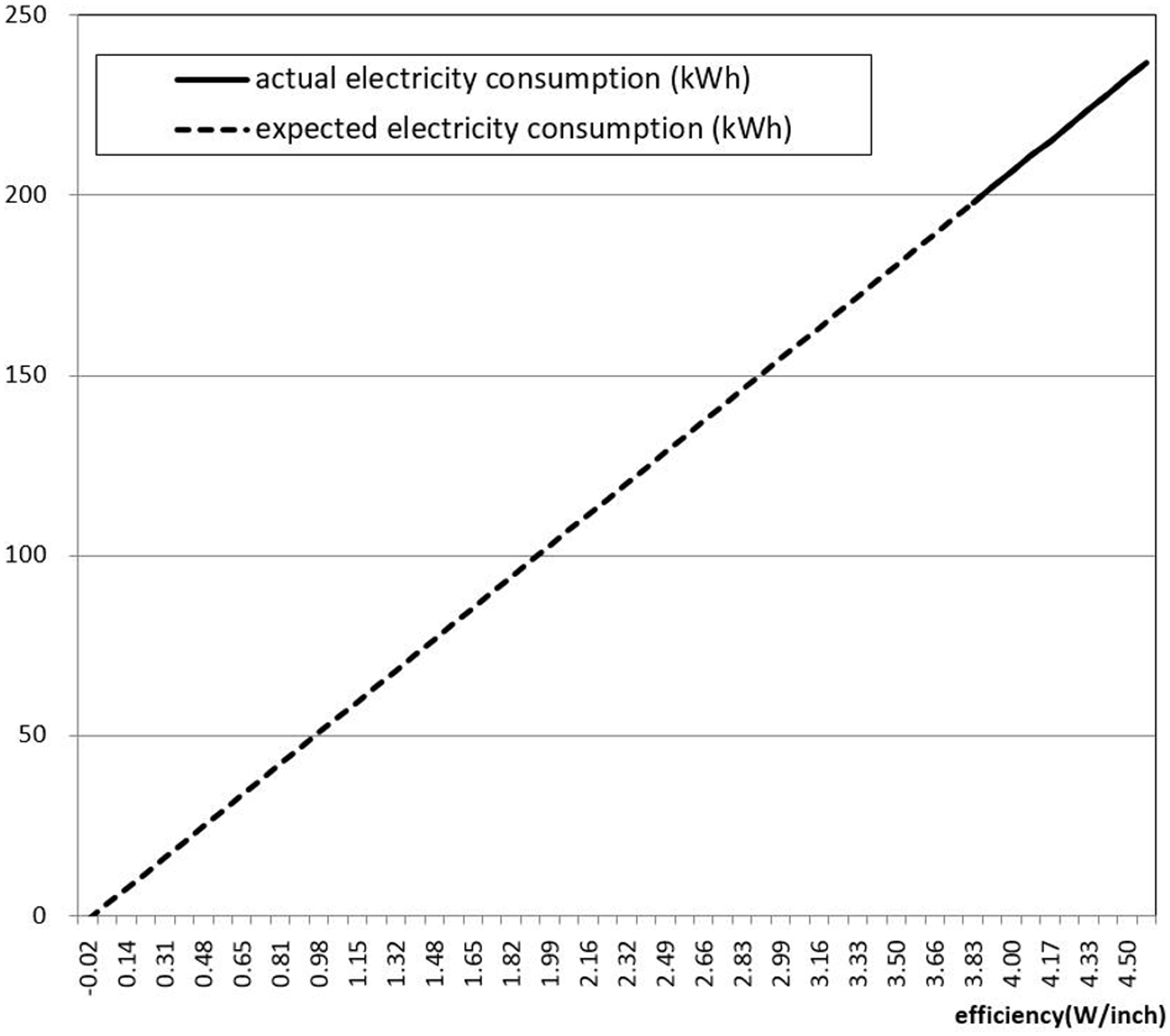
Linear relationship in televisions for low-income households.

Figure 5.

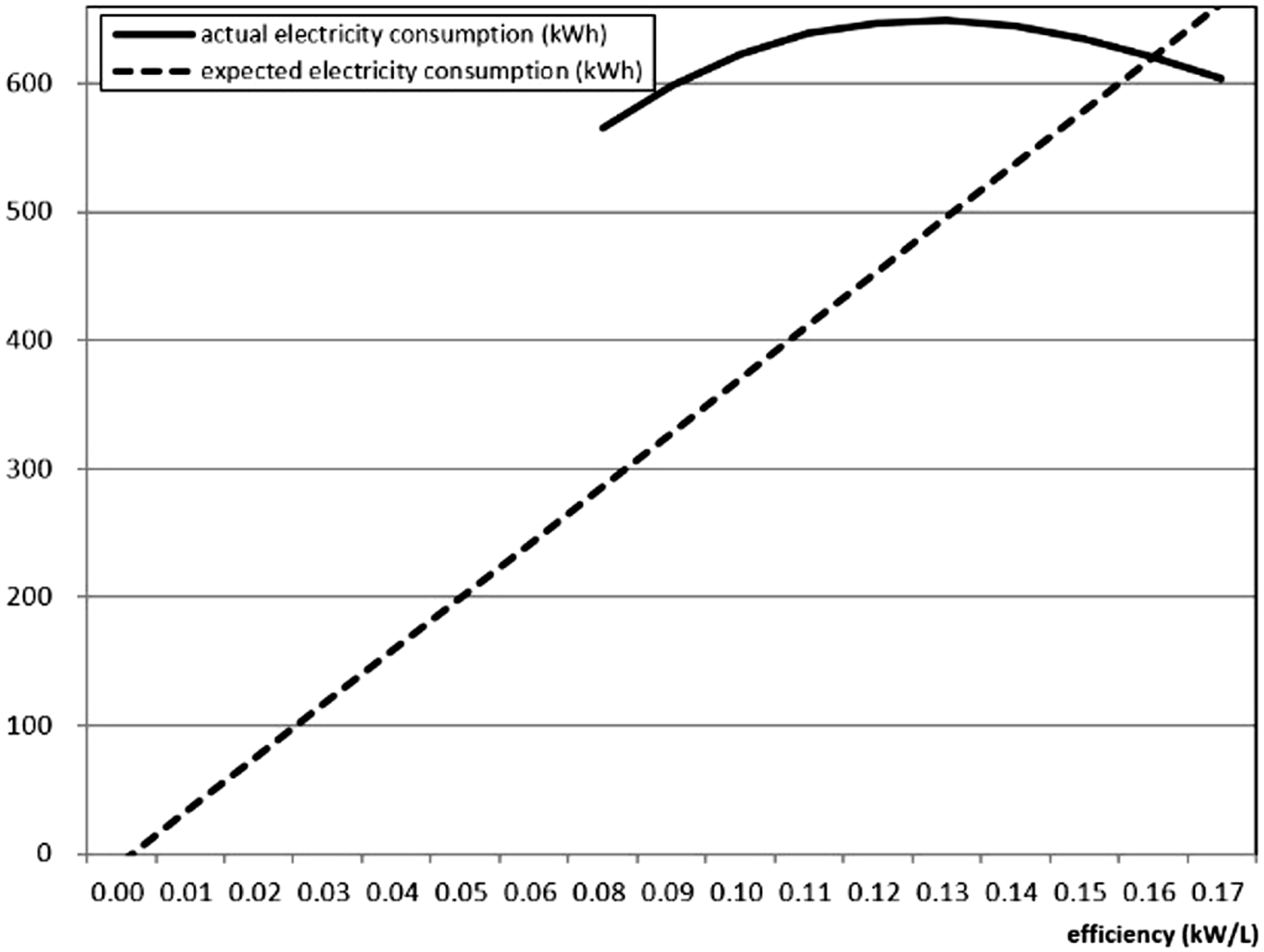
Nonlinear relationship in refrigerators for all-income households. Source: Jin.⁵²

Rebound effects of low-income households in South Korea

Data for low-income and all-income households

In order to estimate the rebound effects of low-income households, raw data from “the Research and Analysis on the Actual Condition of Energy Consumption in Low-income Households” were utilized. The survey was conducted by the Seoul Development Institute to investigate the state of the poor’s energy consumption.⁵⁵ The institute conducted face-to-face interviews of 600 households from 27 July to 7 August 2009. In the survey, the whole area of Seoul was divided into five districts. Each district was allocated 100–150 households depending on their population of low-income households. The survey has the meaning of first face-to-face interviews with low-income households in South Korea.

After the analysis, the results will be compared with those of all-income households provided in the previous study.⁵² The data from “the Survey of Electricity Consumption Characteristics of Home Appliances” were applied to this study.⁵⁶ The survey was conducted by the government-owned company, Korea Power Exchange, to collect basic information about general households’ behavior in energy consumption. The survey has been carried out biennially since 1979. In 2011, the sample size was 4000. Owing to these reasons, the survey is the most credible and official data related to residential electricity consumption. To compare rebound effects with those of low-income households, raw data on 4000 all-income households were utilized in this study.

Jin⁵² estimated rebound effects of home appliances for all-income households analyzing these data. In particular, his study has no theoretical conflict because the author adopted the same method in this study, the modified regression model. Moreover, the comparison is meaningful with regard to time because the periods of the two surveys are not so distant: 2009 and 2011. Therefore, the results from Jin’s study could serve as a proper control group to compare with rebound effects of low-income households.

In this study, three major home appliances were considered: television, refrigerator, and washing machine. These appliances account for 36.2% of electricity consumption in all-income households. The individual percentages of television, refrigerator, and washing machine are 10.4, 23.8, and 2.0%, respectively. In low-income households, these appliances account for 50.6% of electricity consumption. The ratios of television, refrigerator, and washing machine are 15.9, 33.1, and 1.6%, respectively. Overall, the percentage of these basic appliances in energy consumption except for washing machine is larger in low-income households.

Mathematical and graphical results of rebound effects in individual appliances

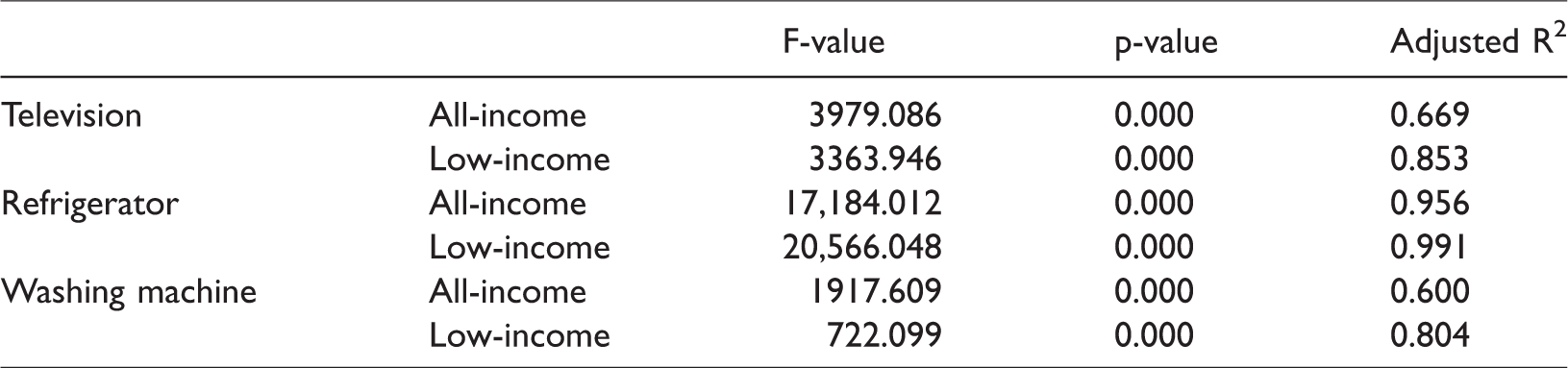
In this subsection, rebound effects for two groups, low-income and all-income households, will be compared. In order to differentiate the results for the two groups, the analyses of home appliances will be individually conducted. Table 1 shows the test statistics of multiple regression in two groups. As a result of the analysis, the F-values are large enough that the model could be validated. In addition, the R² coefficients of determination show the goodness of fit in the multiple regression models. Hereafter, graphs and equations of regression models will be provided to facilitate easy comparison.

Table 1.

Test statistics of multiple regression in two groups.

		F-value	Adjusted R²
Television	All-income	3979.086	0.669
Television	Low-income	3363.946	0.853
Refrigerator	All-income	17,184.012	0.956
Refrigerator	Low-income	20,566.048	0.991
Washing machine	All-income	1917.609	0.600
Washing machine	Low-income	722.099	0.804

First, televisions are important home appliances in everyday life. In the modern society, if it were not televisions, humans nearly could not live. Therefore, most governments have their own public broadcasting system. Equations (4) and (5) indicate that there are linear relationships between efficiency (q) and energy consumption (E_TV) for all-income and low-income households as seen in Figures 3 and 4. These results indicate that there is no rebound effect in both of the groups. Interestingly, while equation (4) for all-income households includes an income variable to control its influence, equation (5) for low-income households excludes the variable because it is not statistically significant. It could be reasonably inferred that an income variable is excluded for low-income households because they are poor

E_{TV_all} = 43 q + 0.95 i

(4)

E_{TV_low} = 51 q

(5)

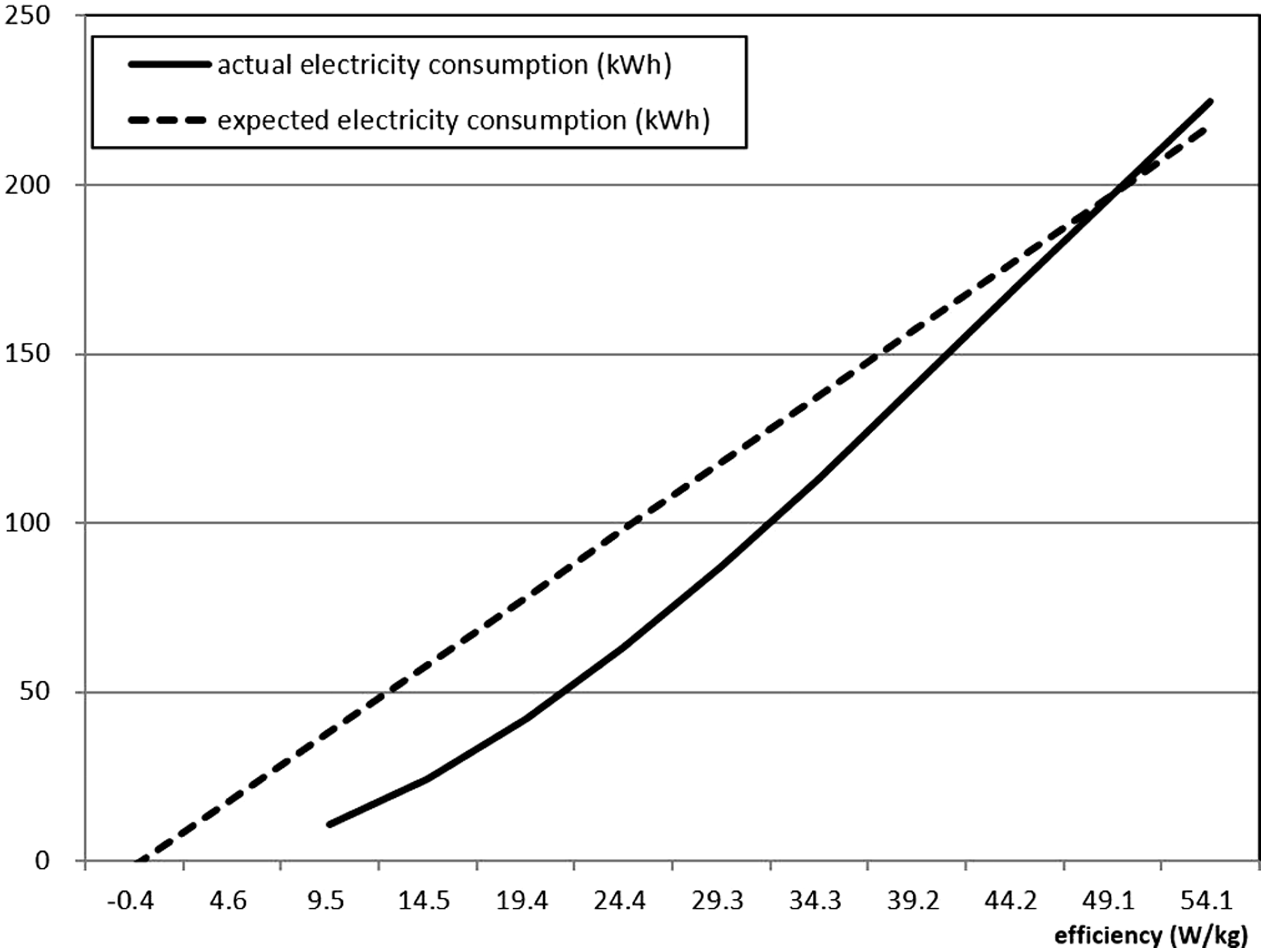
Second, refrigerators have a unique feature from the viewpoint of energy consumption: they operate throughout the year. Therefore, they account for 23.8 and 33.1% of electricity consumption for all-income and low-income households, respectively.⁵⁶ Equations (6) and (7) indicate that there are nonlinear relationships between efficiency (q) and energy consumption (E_ref) for all-income and low-income households as seen in Figures 5 and 6. Similarly to the case of televisions, an income variable is excluded in equation (7) for low-income households because they are economically in the same group

E_{ref_all} = 12143 q - 71178 q^{2} + 126232 q^{3} - 116065 q^{5} + 0.191 i

(6)

E_{ref_low} = 13 q - 0.18 q^{2} + 0.000001 q^{4}

(7)

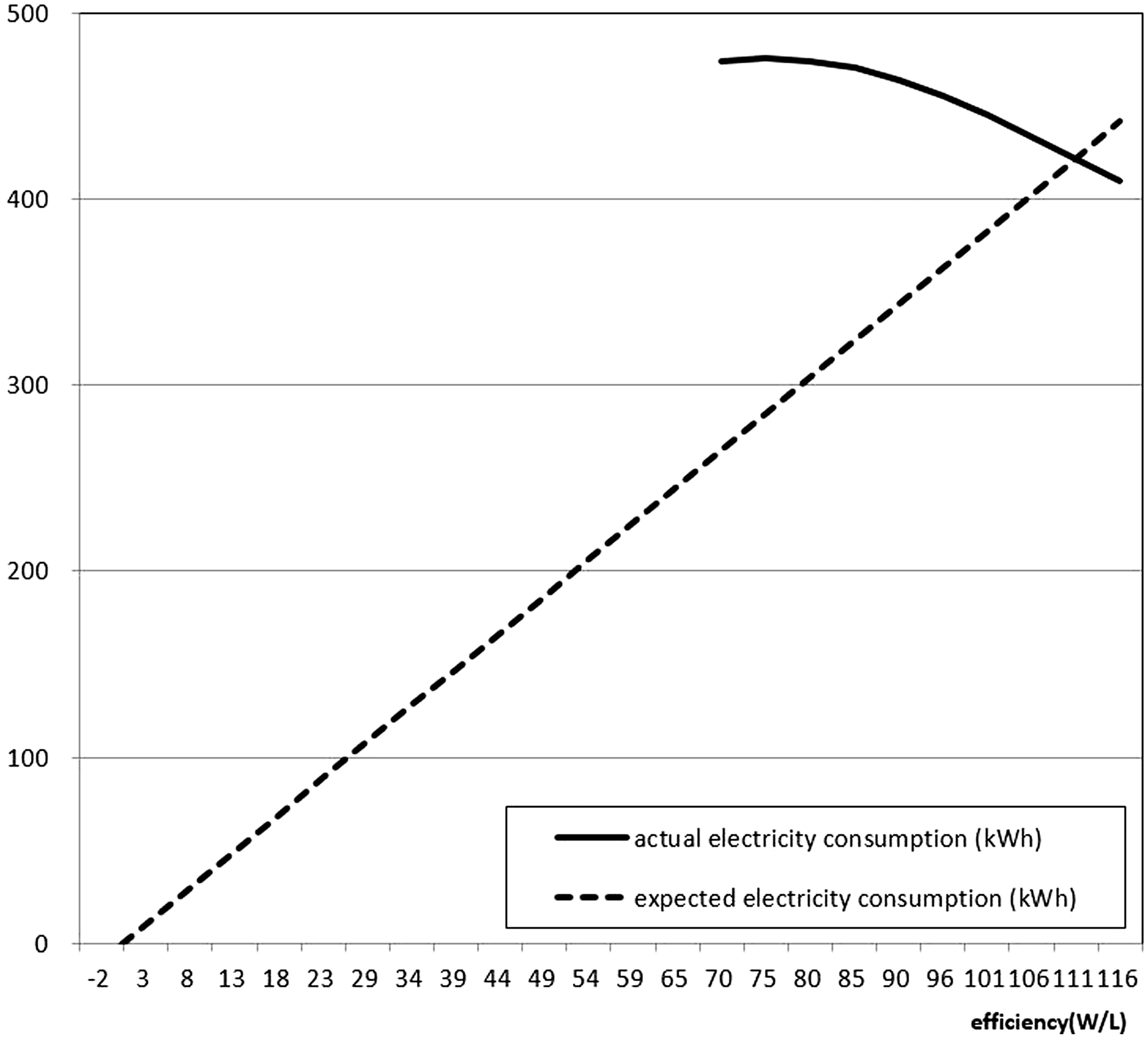
Third, washing machines are one of the necessities in today’s modern life. While only 3.4% of low-income households possess air conditioners, nearly all of them possess washing machines.⁵⁷ Equations (8) and (9) indicate that there are nonlinear relationships between efficiency (q) and energy consumption (E_wash) for all-income and low-income households as seen in Figures 7 and 8. In contrast to televisions and refrigerators, an income variable is included even in the equation for low-income households. This implies that the poor have economic differences even in the same group. In addition, two graphs differently show concave and convex shapes. The specific meaning will be explained in the next subsection

E_{wash_all} = 0.131 q^{2} - 0.001 q^{3} + 0.52 i

(8)

E_{wash_low} = 2.303 q - 1.05 q^{2} + 0.087 i

(9)

Comparison of rebound effects between all-income and low-income households

This study attempts to compare rebound effects between all-income and low-income households for individual home appliances. Two controversies regarding rebound effects were reviewed. The first controversy refers to the magnitude of rebound effects. The estimates indicate that individual home appliances have extremely different values, as observed in Table 2. While rebound effects are zero in the case of television, refrigerators show nearly backfire effects because rebound effects are not less than 100%. In addition, rebound effects for washing machines are extremely different for two groups. To sum up, the magnitude of rebound effects strongly depends on individual appliances.

Table 2.

Rebound effects between all-income and low-income households.

	Rebound effect for all-income households	Rebound effect for low-income households
Television	0%	0%
Refrigerator	83–109%	133–161%
Washing machine	−17 to −35%	211–243%

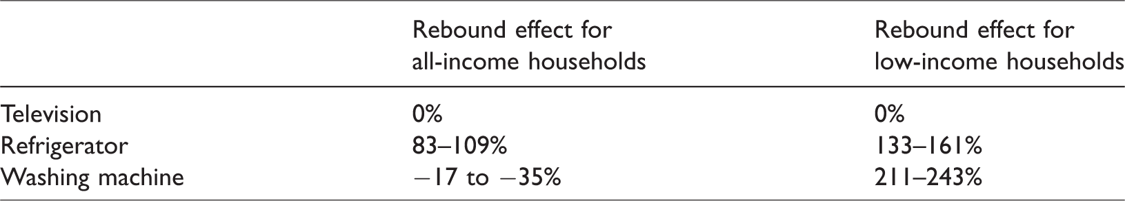
The second controversy related to the influence of income on rebound effects was reviewed. Overall, rebound effects for low-income households are same or larger than the effects for all-income households. In the case of refrigerators, rebound effects are larger for low-income households (133–161%) than for all-income households (83–109%). Finally, while rebound effects of washing machines are negative for all-income households, the estimates for low-income households are tremendous because the effects are more than 200%. Exceptionally, televisions equally have no rebound effect in both groups. Then policy-makers need to introduce efficiency improvement programs of television for low-income households without concerning rebound effects. In particular, these programs could be highly desirable for disabled persons because they spend most of their time watching television. In sum, the differences in rebound effects between all-income and low-income households also depend on individual appliances.

Conclusion and policy implications

The aim of this study was to empirically review the controversies related to rebound effects. Based on the analyses results, three reasonable conclusions were derived. First, rebound effects should be estimated at the micro level. A number of previous studies adopted the elasticity parameter measure to estimate rebound effects. However, this method only shows rebound effects at the macro level, such as private, transportation, and manufacturing sectors. This broad estimation could be useful to understand the basic features of rebound effects in these sectors. However, this estimation is meaningless to policy-makers because governments provide subsidies for individual “equipment,” not for sectors. Therefore, estimation measures at the micro level, such as the regression model, could be helpful to policy-makers.

Second, it is necessary to consider the rebound effects when governments introduce fuel poverty programs because these effects are usually larger for low-income households. This conclusion coincides with most previous studies.⁴⁵ However, policy-makers should also consider the individual differences among home appliances. For example, they do not need to consider the rebound effects of televisions. In contrast, washing machines show totally different rebound effects between all-income households and low-income households. After all, rebound effects of individual appliances are also important even in fuel poverty programs.

Third, rebound effects could have different meanings in fuel poverty programs. Although rebound effects are larger for low-income households, the increase of energy consumption may not be a net loss. When the poor consume more energy after efficiency improvement, these large rebound effects contribute to increasing their amenities. In the real world, most policies have not a single goal, but multiple goals. In the same way, fuel poverty programs have several goals such as energy conservation, greenhouse gases reduction, increase in amenities, and health improvement. While large rebound effects are not desirable from the viewpoint of energy conservation, they are worthwhile with regard to amenity increase. Hence, policy-makers should decide the priority of goals.

Figure 6.

Nonlinear relationship in refrigerators for low-income households.

Figure 7.

Nonlinear relationship in washing machines for all-income households. Source: Jin.⁵²

Figure 8.

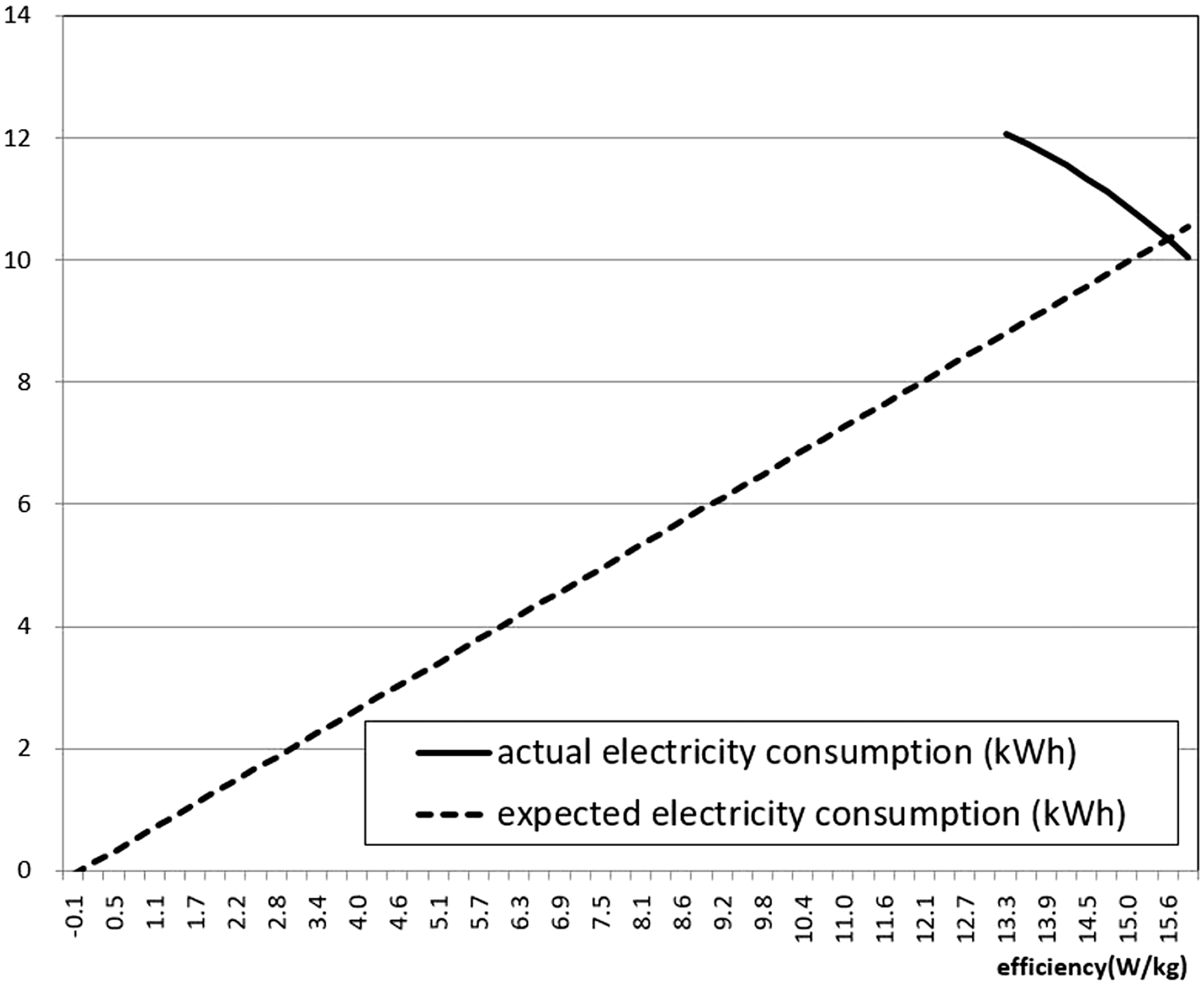
Nonlinear relationship in washing machines for low-income households.

The interest in rebound effects from policy-makers had reached the climax in 2011.⁵⁸ Thereafter, however, the interest has been unfortunately decreased. Partially, insufficient empirical evidence has induced policy-makers’ inaction. The detailed estimates of rebound effects in this study could be useful for policy-makers to introduce efficiency improvement programs as a part of fuel poverty policy.

Nevertheless, this study has six methodological limitations. First, multiple regression analysis, which is critical for the model, is not perfect. Although the values of adjusted R² are relatively high, the analysis still has residuals, that is unexplained parts. In particular, recent studies have revealed that the “intention” for conservation and “behavior” for pro-environmentalism are critical in energy policy.^19,59 In fact, the modified regression model utilizes only two independent variables: efficiency and income. It is necessary to include more various explanatory variables and improve the regression model.

Second, negative values of rebound effects should be illustrated more accurately and evidently. Even the previous studies exemplified super conservation just at the micro level to illustrate this extraordinary phenomenon. Hereafter, theoretical and empirical supports should be supplemented.

Third, the efficiency is difficult to conceptualize. The definition of intensity was used as a substitute for efficiency in this study. However, it is not problematic because intensity of energy is exactly reverse to the concept of efficiency. Therefore, they are compatible with each other. Nevertheless, details of intensity could be debatable. For example, although “watt per inch” was adopted to measure intensity in this study and others, this conceptualization has some flaws because exact intensity means “energy consumption per specific service.” In contrast to refrigerators and washing machines, additional attempts to conceptualize the efficiency or intensity of televisions would be necessary. Likewise, previous studies also have the same problem.⁵⁰

Fourth, cross-sectional data were utilized in this study. However, other studies have made use of time-series data. These data have their own pros and cons. For example, time-series data are good to easily estimate rebound effects using price elasticity. In contrast, they are not proper for individual efficiency improvement programs because their time range is too wide. In spite of this problem, it could be meaningful to apply time-series data for estimation of rebound effects because these data could compensate for the defect of cross-sectional data.

Fifth, the estimated rebound effects are dependent on the points of choice where energy consumption is measured. In order to solve this problem of dependency on the selective choice, rebound effects were suggested in the range. For example, rebound effects were 133–161% in the case of refrigerator for low-income households. Nevertheless, this problem was inevitable because this study adopted the same method with the previous study (Jin, 2019). However, an alternative to solve this problem could be to calculate rebound effects from the area between two graphs: actual electricity consumption and expected consumption.

Sixth, extremely high backfire effects were identified in this study. Particularly, low-income households show highly severe rebound effects as 133–161 and 211–243% for refrigerators and washing machines, respectively. This result is quite exceptional in comparison with the ones from previous studies. Therefore, improvement in methodology would be necessary for identifying the reasons of these severe backfire effects.

Despite these limitations, this study properly conducted the analysis and estimated rebound effects for home appliances. In addition, the study was able to compare rebound effects between all-income and low-income households. Future research should attempt to overcome the limitations by consecutive studies in other countries and in other appliances using different data and methodologies.

Footnotes

Declaration of conflicting interests

The author declared no potential conflicts of interest with respect to the research, authorship, and/or publication of this article.

Funding

The author disclosed receipt of the following financial support for the research, authorship, and/or publication of this article: This work was supported by the Ministry of Education of the Republic of Korea and the National Research Foundation of Korea (NRF-2015S1A2A1A01025901).

Sang-Hyeon Jin is an Associate Professor at School of Public Administration, Kyungpook National University. He worked as researcher at the Seoul Development Institute. He was a visiting scholar at the Center for Energy and Environmental Policy in the College of Arts and Sciences at the University of Delaware. He was also a representative expert of South Korea in the Intergovernmental Panel on Climate Change conference. He specialized in energy policy and climate change policy with a focus on rebound effects.

References

Morvaj

Bukarica

Energy efficiency policy. In: J

Palm

(ed.) Energy efficiency. London, InTech, 2010, pp.1–25.

Thollander

Palm

Rohdin

Categorizing barriers to energy efficiency: an interdisciplinary perspective. In: J

Palm

(ed.) Energy efficiency. London: InTech, 2010, pp.49–62.

Clinch

Healy

Domestic energy efficiency in Ireland: correcting market failure. Energy Policy 2000; 28: 1–8.

Birol

Keppler

JH.

Prices, technology development and the rebound effect. Energy Policy 2000; 28: 457–469.

Brookes

Energy efficiency fallacies revisited. Energy Policy 2000; 28: 355–366.

Loughran

Kulick

Demand-side management and energy efficiency in the United States. Energy J 2004; 25: 19–45.

Heffner

Campbell

Evaluating the co-benefits of low-income energy-efficiency programmes. Paris: International Energy Agency (IEA), 2011.

Missemer

William Stanley Jevons’ The Coal Question (1865), beyond the rebound effect. Ecol Econ 2012; 82: 97–103.

Galvin

The rebound effect, gender and social justice: a case study in Germany. Energy Policy 2015; 86: 759–769.

10.

Galvin

Targeting ‘behavers’ rather than behaviours: a ‘subject-oriented’ approach for reducing space heating rebound effects in low energy dwellings. Energy Build 2013; 67: 596–607.

11.

Greater London Authority (GLA). Fuel poverty in London: Figures and tables illustrating the challenge of tackling fuel poverty. London, UK: The Greater London Authority, 2008.

12.

Department of Environment, Food and Rural Affairs (UK DEFRA). Fuel poverty methodology documentation. London, UK: UK DEFRA, 2006.

13.

Department of Health and Human Services (US DHHS). LIHEAP energy burden evaluation study. New Jersey, US: US DHHS, 2005.

14.

The City of Liverpool. Fuel poverty & warm homes: a strategy for Liverpool. Liverpool, UK: The City of Liverpool, 2007.

15.

Sustainable Energy Ireland (SEI). A review of fuel poverty and low income housing. Dublin, Ireland: Sustainable Energy Ireland, 2003.

16.

Thondhlana

Kua

HW.

Promoting household energy conservation in low-income households through tailored interventions in Grahamstown, South Africa. J Cleaner Prod 2016; 131: 327–340.

17.

Colton

RD.

Energy consumption and expenditures by low-income customers. Electr J. 2002; 15: 70–75. DOI: 10.1016/S1040-6190(02)00279-8.

18.

Kolokotsa

Santamouris

Review of the indoor environmental quality and energy consumption studies for low income households in Europe. Sci Total Environ 2015; 536: 316–330.

19.

James

Ambrose

Retrofit or behaviour change? Which has the greater impact on energy consumption in low income households?

Procedia Eng 2017; 180: 1558–1567.

20.

Jenkins

DP.

The value of retrofitting carbon-saving measures into fuel poor social housing. Energy Policy 2010; 38: 832–839.

21.

Energie-Cities. Action on fuel poverty in social housing. Besançon, France: Energie-Cities, 2007.

22.

Hong

Gilbertson

Oreszczyn

, et al. Ridley I and the Warm Front Study Group. A field study of thermal comfort in low-income dwellings in England before and after energy efficient refurbishment. Build Environ 2009; 44: 1228–1236.

23.

Scott S, Lyons S, Keane C, McCarthy D, , et al. Fuel poverty in Ireland: extent, affected groups and policy issues. ESRI Working Paper No. 262, 2008.

24.

Department of Energy (US DOE). Weatherization assistance program briefing book. Washington DC, US: US DOE, 2008.

25.

Hernandez

Phillips

Benefit or burden? Perceptions of energy efficiency efforts among low-income housing residents in New York City. Energy Res Soc Sci 2015; 8: 52–59.

26.

Bird

Hernandez

Policy options for the split incentive: increasing energy efficiency for low-income renters. Energy Policy 2012; 48: 506–514.

27.

Kaiser

Pulsipher

AG.

The impact of the hold-harmless and give-back provisions on the Low-Income Home Energy Assistance Program allocation mechanism. Energy 2003; 28: 1615–1654.

28.

National Association for State Community Services Programs (NASCSP). Weatherization Assistance Program PY2008 Funding Survey. Washington, DC, US: NASCSP, 2008.

29.

Korea Energy Foundation (KEF). Korea Energy Foundation English Brochure. Seoul, South Korea: KEF, 2010.

30.

Langevin

Gurian

Wen

Reducing energy consumption in low income public housing: interviewing residents about energy behaviors. Appl Energy 2013; 102: 1358–1370.

31.

Yang

Zhao

Do subsidies work better in low-income than in high-income families? Survey on domestic energy-efficient and renewable energy equipment purchase in China. J Cleaner Prod 2015; 108: 841–851.

32.

Agency for International Development (US AID). Proceedings of the workshop: improving electricity service for the urban poor. Washington. DC, US: US AID, 2007.

33.

Korea Energy Foundation (KEF). The web site of the Korea Energy Foundation, www.energylove.org (accessed 14 July 2018).

34.

Gonzalez

JF.

Empirical evidence of direct rebound effect in Catalonia. Energy Policy 2010; 38: 2309–2314.

35.

Sorrell

Improving the evidence base for energy policy: the role of systematic reviews. Energy Policy 2007; 35: 1858–1871.

36.

Dimitropoulos

Energy productivity improvements and the rebound effect: an overview of the state of knowledge. Energy Policy 2007; 35: 6354–6363.

37.

Sorrell

Dimitropoulos

The rebound effect: microeconomic definitions, limitations and extensions. Ecol Econ 2008; 65: 636–649.

38.

Greening

Greene

Difiglio

Energy efficiency and consumption – the rebound effect – a survey. Energy Policy 2000; 28: 389–401.

39.

Grepperud

Rasmussen

A general equilibrium assessment of rebound effects. Energy Econ 2004; 26: 261–282.

40.

Nadel

The rebound effect: large or small. An ACEEE White Paper. Washington, DC: American Council for an Energy-Efficient Economy (ACEEE), 2012.

41.

Saunders

HD.

A view from the macro side: rebound, backfire, and Khazzoom-Brookes. Energy Policy 2000; 28: 439–449.

42.

Galvin

Estimating broad-brush rebound effects for household energy consumption in the EU 28 countries and Norway: some policy implications of Odyssee data. Energy Policy 2014; 73: 323–332.

43.

Khazzoom

JD.

Economic implications for mandated efficiency in standards for household appliances. Energy J 1980; 1: 21–40.

44.

Chakravarty

Dasgupta

Roy

Rebound effect: how much to worry?

Curr Opin Environ Sustain 2013; 5: 216–228.

45.

Madlener

Hauertmann

Rebound effects in German residential heating: do ownership and income matter. FCN Working Paper No. 2/211. Aachen: Institute for Future Energy Consumer Needs and Behavior (FCN), E.ON Energy Research Center, 2011.

46.

Murray

What if consumers decided to all go green? Environmental rebound effects from consumption decisions. Energy Policy 2013; 54: 240–256.

47.

Saunders

HD.

Is what we think of as rebound really just income effects in disguise?

Energy Policy 2013; 57: 308–317.

48.

Chitnis

Sorrell

Druckman

, et al. Who rebounds most? Estimating direct and indirect rebound effects for different UK socioeconomic groups. Ecol Econ 2014; 106: 12–32.

49.

Galvin

Sunikka-Blank

Quantification of (p)rebound effects in retrofit policies – why does it matter?

Energy 2016; 95: 415–424.

50.

Haas

Auer

Biermayr

The impact of consumer behavior on residential energy demand for space heating. Energy Build 1998; 27: 195–205.

51.

Haas

Biermayr

The rebound effect for space heating empirical evidence from Austria. Energy Policy 2000; 28: 403–410.

52.

Jin

SH.

Home appliances’ rebound effects estimated by a modified nonlinear model: an empirical study in South Korea. Energy Efficiency 2019; 12: 2187–2199. DOI: 10.1007/s12053-019-09795-x

53.

Jin

SH.

The effectiveness of energy efficiency improvement in a developing country: rebound effect of residential electricity use in South Korea. Energy Policy 2007; 35: 5622–5629.

54.

Jin

SH.

The effectiveness of energy efficiency improvement program: an analysis of rebound effect in Seoul's low-income household. Korean Policy Sci Rev 2013; 17: 55–77.

55.

Jin

SH.

Dilemma of energy efficiency improvement: market failure, government failure and rebound Effect. In: Jacobs

(ed.) Energy policy: economic effects, security aspects and environmental issues. New York: Nova Science Publisher, 2009, pp.297–308.

56.

Korea Power Exchange (KPX). Survey of electricity consumption characteristics of home appliances. Seoul, South Korea: KPX, 2011.

57.

Jin

SH.

Research and analysis on the actual condition of energy consumption in low-income households. Seoul: Seoul Development Institute, 2009.

58.

Vivanco

Kemp

Voet

How to deal with the rebound effect? A policy-oriented approach. Energy Policy 2016; 94: 114–125.

59.

Chen

Day

JK.

Thermal comfort or money saving? Exploring intentions to conserve energy among low-income households in the United States. Energy Res Soc Sci 2017; 26: 61–71.