Enhancing solar energy integration for hydrogen refueling stations: A novel hybrid forecasting model for accurate DNI prediction in Jiangsu Province

Abstract

Accurate prediction of direct normal irradiance (DNI) is critical for optimizing solar energy integration in hydrogen production systems. This study proposes a novel hybrid forecasting model that integrates variational mode decomposition (VMD), sample entropy (SE), biogeography-based optimization (BBO), and histogram gradient boosting regression (HGBR) to enhance the accuracy of DNI prediction. VMD is used to decompose the nonlinear solar radiation signals, while SE clusters the resulting modes based on complexity. BBO fine-tunes the hyperparameters of HGBR, which serves as the core prediction engine. Applied to a case study in Jiangsu Province, China, the model demonstrates superior forecasting performance compared to conventional models. The proposed hybrid model achieves a coefficient of determination of 0.98 and a root mean square error of 39.69 W/m². The predicted DNI values are used to optimize the design and operation of a solar-powered hydrogen refueling station (HRS), comprising the 1148-kW photovoltaic arrays, a 1000-kW proton exchange membrane, a 204-kWh battery storage system, and a 2000-kg hydrogen storage tank. These forecasts enable dynamic alignment between solar generation and hydrogen production, ensuring energy-efficient scheduling and load management. The techno-economic analysis confirms the system's feasibility, yielding a levelized cost of hydrogen of 3.20$/kg and a net present cost of 2,143,512$. The proposed hybrid model advances forecasting accuracy and can provide a scalable and cost-effective pathway for deploying sustainable hydrogen infrastructure in support of clean transportation.

Keywords

Solar irradiance prediction histogram gradient boosting regression hydrogen refueling station techno-economic analysis Jiangsu Province

Introduction

Growing concerns about climate change, the depletion of fossil fuels, and the negative environmental effects of greenhouse gas (GHG) emissions are causing a significant shift in the global energy landscape.¹ The exponential increase in global energy demand brought on by population growth and industrialization, which severely strains conventional energy sources, adds to this urgency. Unless significant changes are made, the consumption of fossil fuels, in particular, is predicted to increase by about 1.1 million barrels per day by 2025, indicating a continued reliance on carbon-intensive energy sources.² Because internal combustion engine (ICE) vehicles continue to dominate the market despite their substantial contribution to carbon emissions and air pollution, the transportation sector continues to play a significant role in this trend. Clean energy alternatives like battery electric vehicles (BEVs) and, more significantly, fuel cell electric vehicles (FCEVs), which run on hydrogen fuel and only emit water vapor, are becoming more and more popular in response.^3,4

Hydrogen refueling stations (HRSs), which are essential infrastructures for storing and delivering hydrogen fuel to vehicles, are a major requirement for FCEVs.^5,6 Despite their significance, there is still a lack of global HRS deployment, which prevents FCEVs from being widely adopted.^7,8 Governments all around have taken strong action to hasten the development of hydrogen infrastructure in recognition of this. This global change is exemplified by the U.S. H2@Scale program, Japan's H2 Mobility initiative, and China's hydrogen development roadmap, which aims to produce over 50,000 hydrogen vehicles.^9–11 The on-site production of green hydrogen using renewable energy, especially solar photovoltaics (PV), is one of the most promising innovations in this field. It improves sustainability and lessens dependency on grid electricity.¹² However, this integration adds new technical and financial challenges because solar energy is intermittent, and FCEV users’ refueling habits are unpredic table.¹³

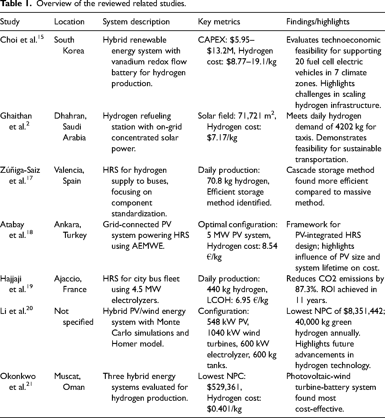
With the development of techno-economically optimized HRSs driven by hybrid renewable energy systems, recent studies have made notable progress in tackling these issues.^14–21 Key performance metrics like CAPEX, levelized cost of hydrogen (LCOH), and hydrogen production efficiency are highlighted in these works, which use a variety of techniques, including mixed-integer linear programming models, multi-objective optimizations, and HOMER simulations. Although Table 1 summarizes a significant drawback that most of these studies have in common is the lack of a reliable, accurate method for predicting direct normal irradiance (DNI), a critical parameter for solar hydrogen production.

Table 1.

Overview of the reviewed related studies.

Study	Location	System description	Key metrics	Findings/highlights
Choi et al.¹⁵	South Korea	Hybrid renewable energy system with vanadium redox flow battery for hydrogen production.	CAPEX: $5.95–$13.2M, Hydrogen cost: $8.77–19.1/kg	Evaluates technoeconomic feasibility for supporting 20 fuel cell electric vehicles in 7 climate zones. Highlights challenges in scaling hydrogen infrastructure.
Ghaithan et al.²	Dhahran, Saudi Arabia	Hydrogen refueling station with on-grid concentrated solar power.	Solar field: 71,721 m², Hydrogen cost: $7.17/kg	Meets daily hydrogen demand of 4202 kg for taxis. Demonstrates feasibility for sustainable transportation.
Zúñiga-Saiz et al.¹⁷	Valencia, Spain	HRS for hydrogen supply to buses, focusing on component standardization.	Daily production: 70.8 kg hydrogen, Efficient storage method identified.	Cascade storage method found more efficient compared to massive method.
Atabay et al.¹⁸	Ankara, Turkey	Grid-connected PV system powering HRS using AEMWE.	Optimal configuration: 5 MW PV system, Hydrogen cost: 8.54 €/kg	Framework for PV-integrated HRS design; highlights influence of PV size and system lifetime on cost.
Hajjaji et al.¹⁹	Ajaccio, France	HRS for city bus fleet using 4.5 MW electrolyzers.	Daily production: 440 kg hydrogen, LCOH: 6.95 €/kg	Reduces CO2 emissions by 87.3%. ROI achieved in 11 years.
Li et al.²⁰	Not specified	Hybrid PV/wind energy system with Monte Carlo simulations and Homer model.	Configuration: 548 kW PV, 1040 kW wind turbines, 600 kW electrolyzer, 600 kg tanks.	Lowest NPC of $8,351,442; 40,000 kg green hydrogen annually. Highlights future advancements in hydrogen technology.
Okonkwo et al.²¹	Muscat, Oman	Three hybrid energy systems evaluated for hydrogen production.	Lowest NPC: $529,361, Hydrogen cost: $0.401/kg	Photovoltaic-wind turbine-battery system found most cost-effective.

For solar-powered HRSs to be designed and operated dependably, accurate DNI forecasting is necessary.^22,23 Without it, the demand for hydrogen is not met by energy production, which can result in supply shortages, energy waste, or operational inefficiencies.^24,25 Machine learning (ML) and deep learning (DL) approaches like artificial neural networks (ANNs),²⁶ long short-term memory networks (LSTMs),²⁷ gated recurrent units (GRUs),²⁸ and hybrid combinations involving genetic algorithms or reinforcement learning^29–33 are the main methods used in current research in solar irradiance forecasting. Even though these models are better than conventional statistical models, they frequently undervalue the significance of data preprocessing methods that can deal with the non-linearity and non-stationarity that are inherent in data on solar radiation. Furthermore, there is a significant research gap because few studies directly connect their forecasting models to real-world energy applications like HRS design.

The potential of hybrid models that combine optimization and decomposition with sophisticated regressors has been demonstrated by some recent attempts. For instance, Jacques Molu et al.³³ proposes a new method for short-term solar irradiance forecasting, combining Bayesian optimized attention-dilated LSTM with Savitzky–Golay filtering. Applied to data from Douala, Cameroon, the approach enhances data quality and forecasts accuracy. Among several models, the proposed method, integrating attention mechanisms and dilated convolutional layers, showed the best performance with a symmetric mean absolute percentage error of 0.6564. This work introduces novel data processing techniques and a hybrid deep learning model, improving solar irradiance forecasting for researchers and solar plant managers. Gao et al.³⁴ suggest a deep forecasting strategy that utilizes a convolutional neural network (CNN) and LSTM to accurately estimate solar irradiance in a variety of locations. It is underscored that the precision of forecasts can be improved by decomposing the data. Puah et al.³⁵ employ an artificial neural network and exponential smoothing to estimate solar irradiance, utilizing the long-term recording data and timestamp. It is believed that the problem can be considerably simplified by decomposing solar data based on its relevance to trends. Lee et al.³⁶ propose four joint models to mitigate the variability of the solar irradiance prediction error.

Although forecasting solar radiation using individual ML or DL models has advanced significantly in the literature, a major drawback is the fragmentation of approaches. The majority of earlier research on solar irradiance prediction used separate parts, like regressors, optimization algorithms, or decomposition techniques, without integrating them into a cohesive, cooperative pipeline that captures the intricacy and dynamic nature of actual energy systems. This disparity is particularly important for solar-to-hydrogen applications, where cost-effectiveness, operational efficiency, and optimal system design depend on accurate and flexible forecasting. The incorporation of sophisticated computational methods is still mainly unexplored in this field. A forecasting architecture that not only increases accuracy but also fits the financial and practical limitations of hydrogen refueling infrastructure is vitally required. In order to bridge this gap, this study suggests a brand-new hybrid forecasting model, which is a coherent fusion of four different but complementary approaches: ensemble regression learning, entropy-based clustering, signal decomposition, and metaheuristic optimization. Each of these methods addresses a distinct problem related to the prediction of solar irradiance by adding a specific function to the model.

The first preprocessing approach is variational mode decomposition (VMD), which addresses the inherent nonlinearity and non-stationarity of solar radiation data by decomposing the original time series into a finite number of intrinsic mode functions (IMFs). By removing high-frequency noise and isolating oscillatory components, VMD reveals meaningful patterns in both the temporal and frequency domains.^37,38 In contrast to traditional decomposition methods, VMD offers better control over the number of components extracted, reduced mode mixing, and improved stability^39–41—all of which are crucial when dealing with highly variable atmospheric conditions that affect DNI readings. As a result, VMD improves the interpretability and tractability of the raw input data. The model uses sample entropy (SE) after decomposition to measure each IMF's complexity. This stage is essential for separating signal components with significant patterns from those that are primarily random or redundant. SE facilitates dimensionality reduction while maintaining the most informative features by grouping components with comparable entropy value.^42,43 This step sharpens the downstream predictive model's learning focus while simultaneously enhancing computational efficiency. Crucially, this complexity-aware feature selection prevents the forecasting model from overfitting to trivial fluctuations or noise.

Biogeography-based optimization (BBO), a metaheuristic algorithm influenced by the migration and distribution patterns of biological species across ecosystems, is incorporated into the model to further improve predictive performance. By balancing exploration and exploitation throughout the search space to prevent local minima, BBO is used to adjust the learning model's hyperparameters. BBO optimizes the histogram gradient boosting regressor (HGBR) parameters in this study, including learning rate, number of estimators, and tree depth. BBO offers a more flexible and biologically inspired exploration mechanism than grid search or random search techniques,^44–46 making it ideal for intricate, multimodal optimization issues like solar forecasting. Through its integration, the regression model is ensured to function with optimal accuracy, customized to the unique features of the dataset.

The HGBR, a powerful ensemble learning algorithm known for its effectiveness with large data sets, noise tolerance, and potent generalization powers, is at the core of the model.^47,48 In a sequential fashion, HGBR builds several decision trees, each of which fixes the mistakes of the one before it.⁴⁹ In contrast to conventional gradient boosting, HGBR uses histogram-based binning, which reduces computation time without sacrificing accuracy. Because speed and accuracy are essential in energy systems, it is perfect for real-time or near-real-time forecasting applications. The final model achieves a high degree of predictive power with low overfitting risk by optimizing it with BBO and applying HGBR to the entropy-filtered VMD components.

The methodologically cohesive integration of VMD, SE, BBO, and HGBR into a single, fully optimized forecasting pipeline, rather than their separate application—all of which have been used in previous works—is what sets this study apart. In the context of DNI forecasting for solar-powered hydrogen refueling stations, this study is the first to combine these four methods. The strength of the model is its modular design, in which every component strengthens a particular shortcoming of conventional models, compounding the improvement in overall performance. Furthermore, this model has been meticulously developed with practical application in mind, making it more than just theoretical in nature. In particular, it is incorporated into the planning and design of a hydrogen refueling station (HRS) in Jiangsu Province, China, an area with a variety of climates and a rising need for transportation options powered by renewable energy. The VMD-SE-BBO-HGBR model's predicted DNI values are crucial in this scenario because they inform the HRS's operational strategy, which consists of a battery energy storage system to balance load variability, a PV power generation system, and a proton exchange membrane (PEM) electrolyzer for hydrogen production. In order to optimize energy conversion efficiency and ensure a more stable and responsive hydrogen supply chain, the station can dynamically modify hydrogen production schedules to correspond with real-time solar availability by integrating precise solar irradiance forecasting into the core of system management. The integration of advanced hybrid models with renewable infrastructure to improve the responsiveness, flexibility, and sustainability of hydrogen energy systems is an example of a larger systems-level innovation that goes beyond predictive accuracy. In order to reduce the risks associated with intermittency and demand fluctuations, the forecasting model also aids in strategic decision-making regarding energy dispatching, component sizing, and storage utilization. The HRS case study provides a concrete illustration of how forecasting tools can enable new performance and resilience levels in clean energy applications when they are properly customized and integrated into system architecture. By doing this, the research can establish the foundation for wider replication in other technical and geographic contexts where hydrogen infrastructure is being investigated or developed. Thus, this work offers the following dual contributions to the field:

Through the methodical integration of decomposition, clustering, optimization, and ensemble regression, this study presents a unified and modular hybrid model that addresses significant shortcomings of current forecasting techniques.

The model is implemented and validated within a fully designed, renewable-powered HRS, addressing the gap between algorithmic development and real-world energy systems from the standpoint of practical application.

Together, these contributions represent a significant advancement in both the theory and practice of solar energy integration, which can offer a replicable framework for optimizing renewable hydrogen infrastructure worldwide. The study's remaining portions are as follows: The dataset and case study description are given in Section “Case study.” The methodology is presented in Section “Methodology.” Results and discussions are provided in Section “Results and discussions.” The conclusion is offered in Section “Conclusions.”

Case study

Study area and data description

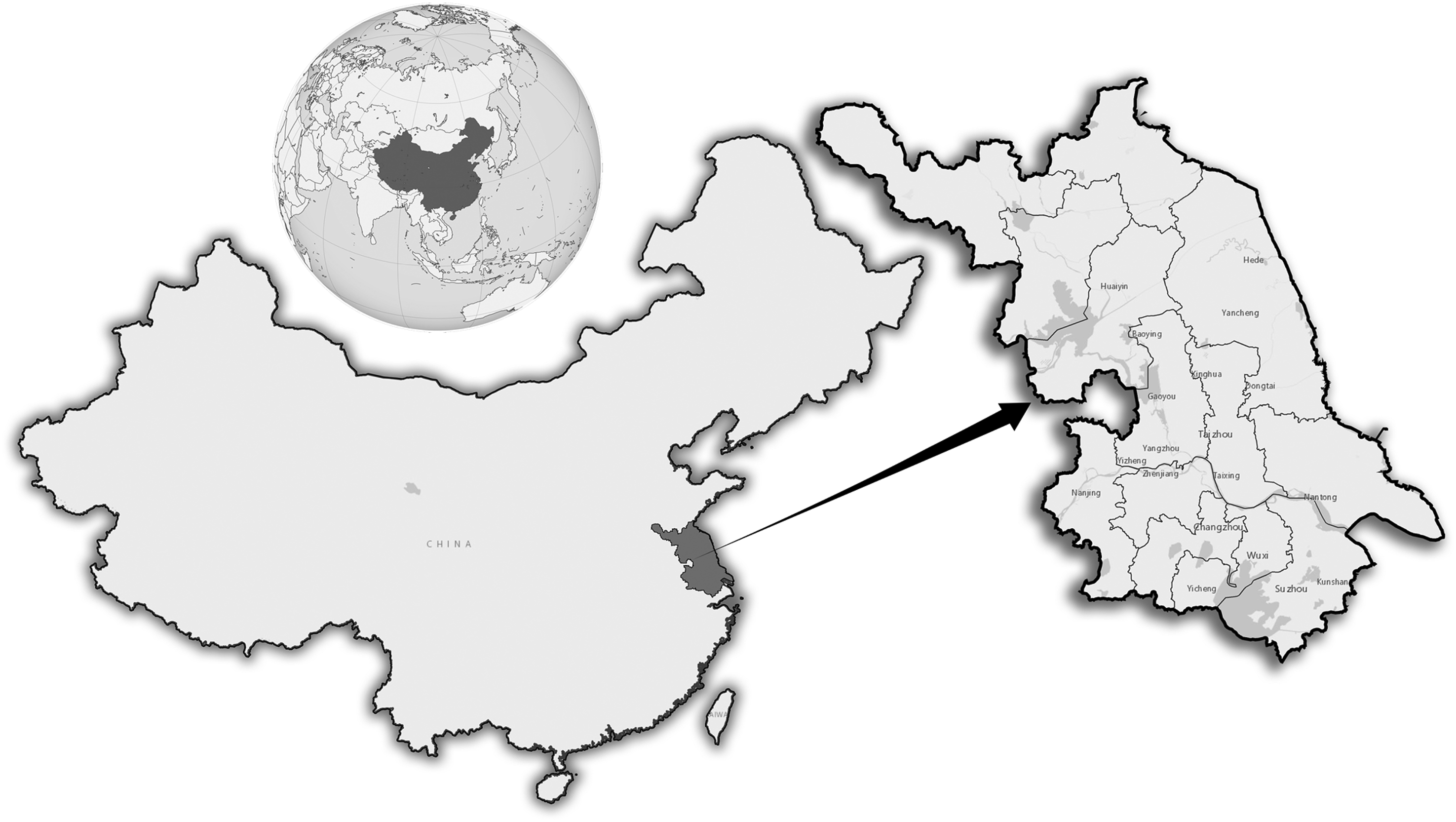
Jiangsu is a province located on the east coast of China which has illustrated in Figure 1. The location's latitude and longitude are $32.6865 \circ N$ and $119.9041 \circ E$ . The climate of Jiangsu is generally known as a subtropical monsoon climate with four seasons. Jiangsu's summer from June to August is typically hot and muggy, with temperatures between 25 °C and 35 °C. At this time, there is a chance of rain and cloudy weather. The weather in Jiangsu in autumn is mild and pleasant. The temperature gradually decreases. The temperature ranges from 15 °C to 25 °C. Winter in Jiangsu ranges from 0 to 10 °C. Snowfall is not common, but sometimes it may occur in the northern areas of this province. Spring starts from March to May in Jiangsu with mild temperatures ranging from 10 °C to 20 °C. More rain can be seen in this season.⁵⁰

Figure 1.

Illustration of the Jiangsu map.

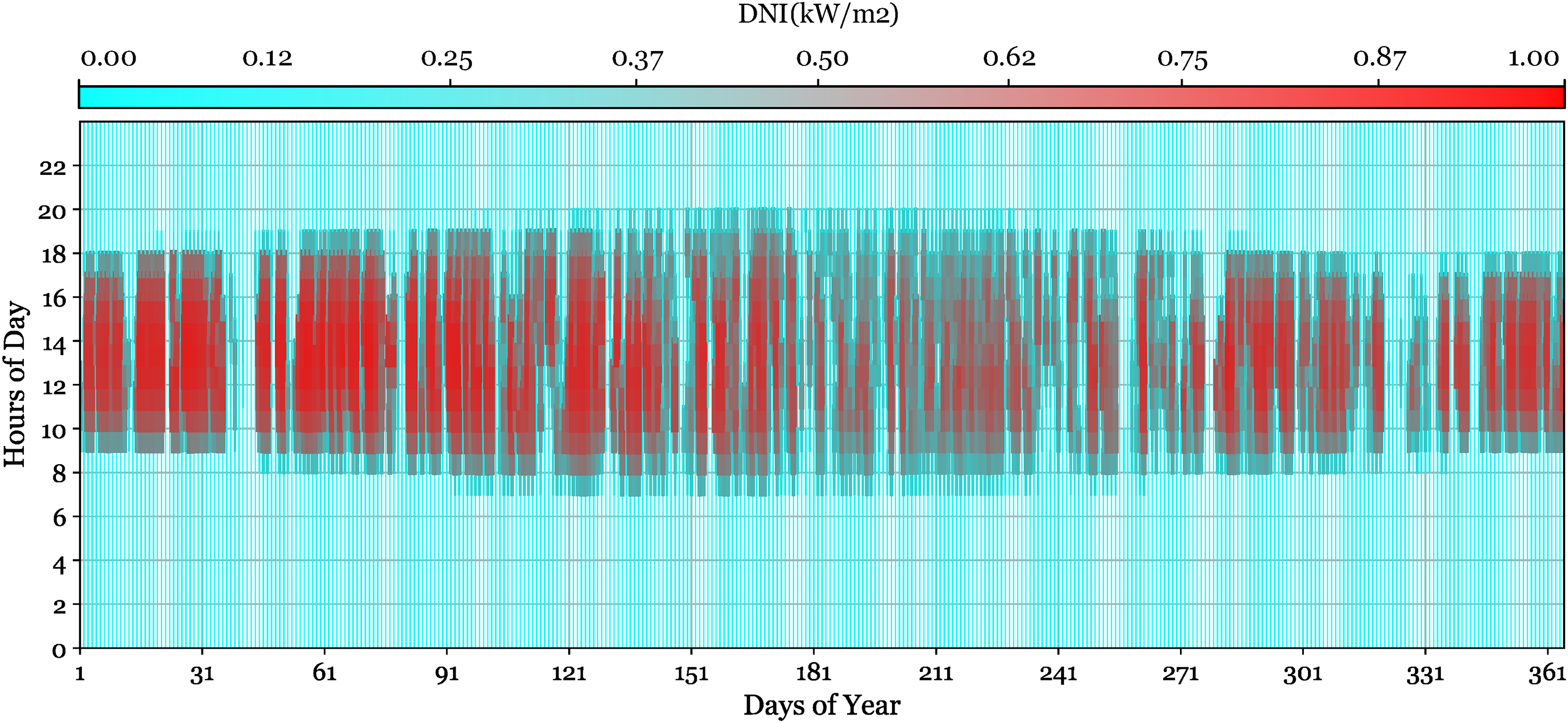
Table 2 provides an overview of the key meteorological variables collected from Jiangsu City, which are critical for developing accurate solar irradiance forecasting models. These variables include temperature, relative humidity, dew point, precipitation, cloud cover, diffuse radiation, wind speed, wind direction, wind gusts, and DNI. The DNI is a vital metric for solar forecasting, is measured in $(W / m^{2})$ and serves as the primary target variable for prediction in this study. Other meteorological parameters, such as temperature $(\circ C)$ , relative humidity $(%)$ , and cloud cover $(%)$ , act as influential predictors, capturing the dynamic and multifactorial nature of weather conditions in Jiangsu's subtropical monsoon climate. The data were collected over diverse seasonal conditions in Jiangsu City, characterized by its four distinct seasons. The inclusion of such comprehensive and diverse variables facilitates the development of a robust forecasting model.

Table 2.

Overview of variable data obtained from Jiangsu City.

Feature	Abbreviation	Units
Temperature	Temp	$(\circ C)$
Relative Humidity	RH	$(%)$
Dew Point	Dew	$(\circ C)$
Precipitation	PRC	$(mm)$
Cloud Cover	CC	$(%)$
Diffuse Radiation	DHI	$(W / m^{2})$
Wind Speed	WS	$(km / h)$
Wind Direction	WD	$(\circ N)$
Wind Gusts	WSG	$(km / h)$
Direct Normal Irradiance	DNI	$(W / m^{2})$

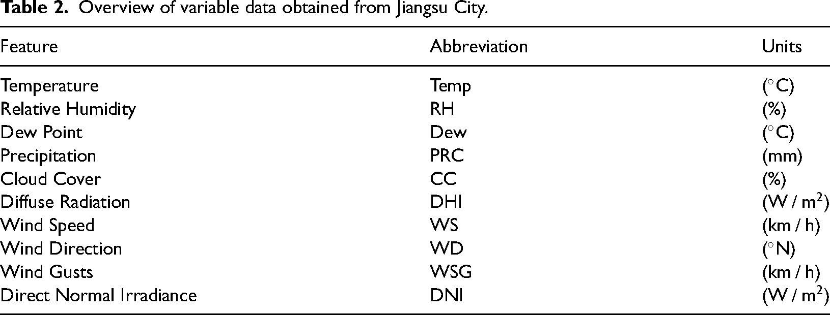
The solar irradiance dataset evaluated in this study gives a complete perspective of the region's DNI across a year, as depicted in Figure 2. The data provide hourly DNI measurements, an important metric for creating solar forecasting models. As demonstrated in Figure 2, the yearly fluctuation in DNI is displayed against the days of the year and hours of the day. The visualization of DNI demonstrates Jiangsu's distinctive climatic dynamics, including the fluctuation owing to seasonal variations in temperature, cloud cover, and precipitation.

Figure 2.

Hourly direct normal irradiance data for the site location over a year.

Feature selection

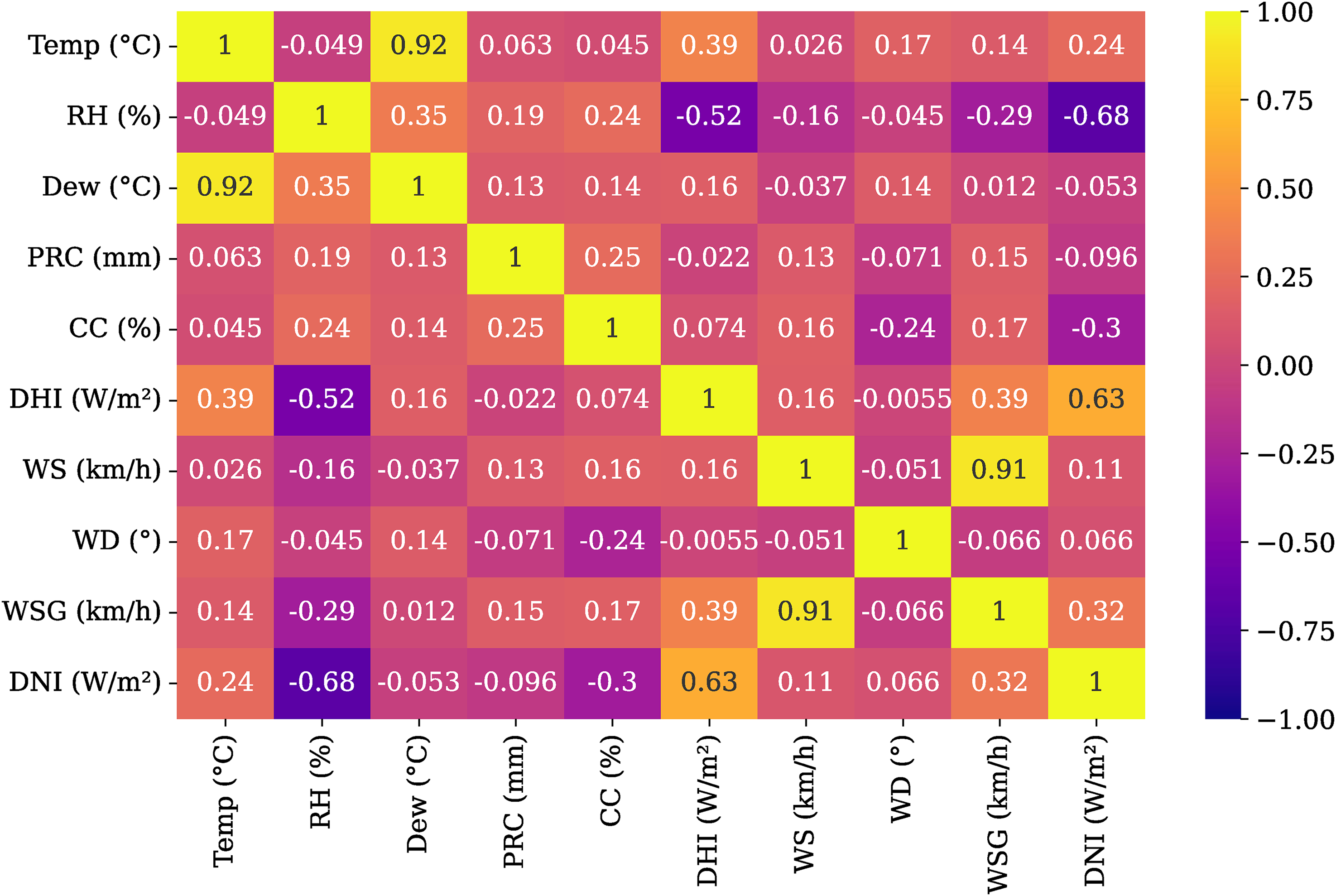
The correlation of DNI with the variables RH, Dew, RRC, CC, DHI, WS, WD, WSG, DNI, and Temp was investigated with the Pearson correlation test and illustrated by Figures 3 and 4. Variables that exhibited no significant correlation were excluded, while those demonstrating a significant correlation were retained for inclusion as input variables. Variables with correlation values ranging from −0.2 to 0.2 were considered to have a negligible relationship with DNI and were consequently removed. Specifically, Dew, WS, PRC, and WD were excluded due to their relatively weak correlation with DNI.

Figure 3.

Heat map illustration showing variable correlation.

Figure 4.

The correlations and distribution of the data.

A statistical metric that assesses the linear relationship among two variables that are continuous is the Pearson correlation, frequently referred to as Pearson's correlation coefficient or Pearson's r. This measure is represented by a numeric value between −1 and 1, where the magnitude and direction of the correlation between the variables are indicated. The proportional connection among the two variables is measured by the Pearson correlation coefficient. When the coefficient is close to 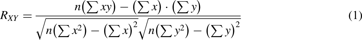$+ 1$ , it indicates a strong positive correlation, meaning that as one variable increases, the other variable also tends to increase in direct proportion. Conversely, a coefficient closes to $- 1$ indicates a significant negative correlation, suggesting that as one variable increases, the other variable typically decreases in proportion. When the value of the coefficient is close to 0, the linear connection between the two variables is insufficient or absent, which means that modifications in one variable do not always coincide with changes in the other. The Pearson's correlation coefficient (R) of two supplied variables X and Y is calculated using the following equation⁵¹

R_{X Y} = \frac{n (\sum x y) - (\sum x) \cdot (\sum y)}{\sqrt{n (\sum x^{2}) - {(\sum x)}^{2}} \sqrt{n (\sum y^{2}) - {(\sum y)}^{2}}}

(1)

Figure 3 presents a heat map that visually illustrates the Pearson correlation coefficients among the variables under investigation, including Temp, RH, Dew, PRC, CC, DHI, WS, WD, WSG, and DNI. The heat map represents the strength and direction of the correlations, with yellow shades denoting strong positive correlations and purple shades indicating strong negative correlations. Several key relationships, such as the strong positive correlation between DNI and Temp (R = 0.63) and the notable negative correlation between DNI and RH (R = −0.68) are highlighted. Conversely, variables such as Dew, PRC, WS, and WD exhibit negligible correlations with DNI (R values ranging from −0.2 to 0.2), indicating a lack of significant linear relationships. These weaker correlations informed the feature selection process, leading to the exclusion of these variables from further modeling efforts.

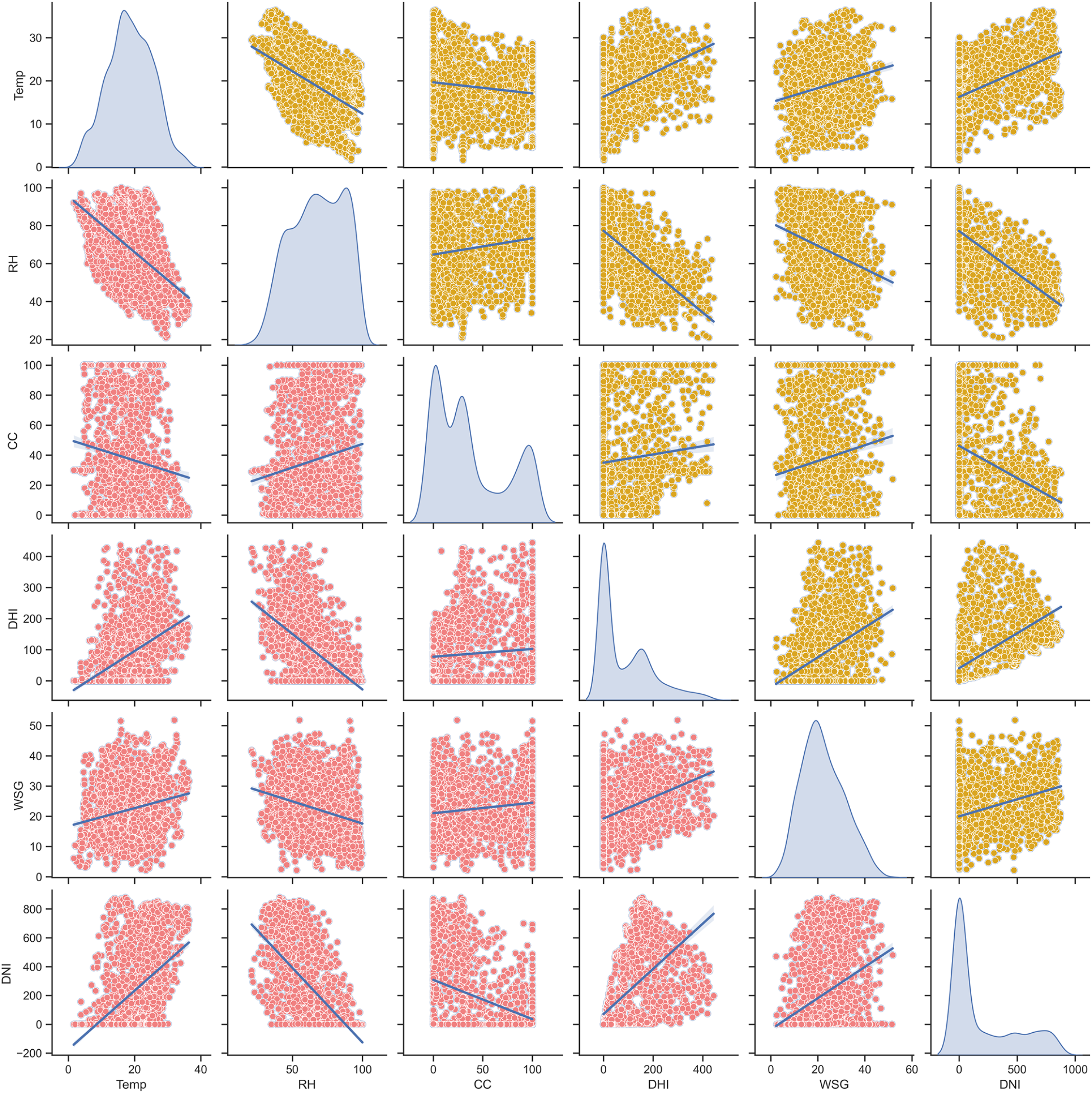
Figure 4 displays a matrix of scatterplots and histograms, providing a comprehensive view of the pairwise relationships and distributions of the selected variables. Each scatterplot visually demonstrates the linear relationship between two variables, complemented by a regression line to indicate the trend. Diagonal elements of the matrix represent the univariate distributions of each variable through kernel density plots, offering insights into the spread and central tendency of the data. Figures 3 and 4 provide a robust framework for analyzing variable correlations and distributions, facilitating informed decisions during the feature selection process for the DNI forecasting model.

Electric and hydrogen demand load

Jiangsu Province served as the research location. Consequently, a crucial component of this study has been estimating the demand for electricity and hydrogen in order to evaluate the operational needs of the suggested HRS. Reports from the regional government and anticipated FCV deployment scenarios in Jiangsu were used to calculate the hydrogen demand numbers. With a fleet of roughly 40–50 light-duty FCVs, each requiring 2–2.5 kg of hydrogen per day, the assumed average daily hydrogen consumption of 100 kg is equivalent. A high-throughput refueling scenario is reflected in the peak hydrogen load of 18.04 kg/hr, ensuring that the station design can handle surge demand during periods of peak operation. In keeping with Jiangsu's roadmap for the development of hydrogen energy, this estimate creates a realistic and scalable demand profile. The electrical consumption of different components, such as compressors and auxiliary equipment necessary for the station's operation, is also included in the hydrogen load profile. The load factor, which is the ratio of average to peak load, is 0.23, indicating moderate variability in hydrogen use, and the average hydrogen demand of 100 kg/day is equivalent to 4.17 kg/hr. The majority of the electrical load comes from auxiliary systems used in the compression and distribution of hydrogen. A variety of subsystems rely on the conversion of AC power into DC. With an hourly average of 3.16 kW, the average daily electric demand is 75.9 kWh. With an electric load factor of 0.25 and a maximum electric load of 12.46 kW during peak refueling activity, the energy consumption appears to be comparatively stable with sporadic spikes. The station's overall design incorporates these demand profiles to support scalability for projected increases in hydrogen consumption and ensure dependable operation in both average and peak operations. The larger objective of facilitating the development of sustainable hydrogen infrastructure in Jiangsu Province is supported by this thorough energy assessment.

Methodology

SARIMAX

SARIMAX is an extended version of the ARIMA model, considering that the seasonality in the time series data may be influenced by other external factors. It is now extensively used and integrates all the major properties of autoregression with moving averages, with the possibility of incorporating exogenous variables for greater precision.⁵² Fundamentally, the SARIMAX accounts for both internal patterns of the time series data and external causes of variation. The autoregressive part models the relation of the current observation and past data points, while the moving average component focuses on the dependency from the previous errors or shocks that the current value depends upon. The time series data needs to be stationary; hence, the integration part of the model applies differencing.⁵³ It includes the basic SARIMA model and adds to it the possibility of inclusion of external factors. This model, by including such additional variables, allows taking care of the problems of autocorrelation, thus making the model even better with respect to forecasts and forecast errors. By allowing the addition of these exogenous variables, greater sophistication is allowed; this permits a more accurate reflection of the real underlying pattern of the data. These exogenous variables can represent a variety of factors that influence the data but are not part of the primary time series itself. For example, they may include external time series data that are related to the primary series, such as weather conditions. It is crucial to accurately predict these external factors in advance, as they play a significant role in the model's performance. The SARIMAX model effectively integrates those additional exogenous inputs into the refinement of its predictions. Considering exogenous variables, it enhances the model to capture complex patterns or improves forecasting accuracy. Therefore, the SARIMAX can very well turn out to be an important tool for the prediction of seasonal temporal data resulting from external influences.⁵³

Gated recurrent unit

The GRU is a type of RNN architecture used primarily for sequence modeling and prediction tasks. The main objective behind developing the GRU was to address some of the limitations posed by the vanishing gradient problem, which can hinder the performance of traditional RNNs.^54,55 However, the GRU model, despite its merits, did not always turn in performances as expected in some applications, while in contrast, the HGBR model has proved to give more positive and acceptable results in certain scenarios. GRU was hence introduced by Kyunghyun Cho as a solution to computational load issues that could lead to delays when using LSTM networks. Unlike LSTMs, which have three gates (input, forget, and output), a standard GRU combines the forget and input gates into two simplified gates: the reset gate and the update gate.⁵⁶ This simplification reduces the model's complexity; hence, GRUs are faster and less computationally intensive compared to LSTMs. However, this means GRUs might not be that powerful and effective in solving certain complex problems because of their simpler structure. The GRU is represented by two key gates: the reset gate, which helps in deciding how much of the previous hidden state to forget, and the update gate, which will determine how much of the new information should be passed forward.⁵⁶ These gates work together to update the network's state in a more efficient manner than traditional RNNs, though they are not always the best fit for every task. Despite its computational efficiency, the GRU-based systems are not suitable for all types of problems. The simplicity of the architecture, while beneficial in terms of speed, may limit the model's ability to capture the complexity of certain data patterns, leading to suboptimal performance in some use cases.

Histogram gradient boosting regressor

HGBR refers to a machine learning technology that combines the ideas of gradient boosting with a histogram-based approach for feature division and orients it to perform regression tasks. It is an adaptation of the well-known method known as the gradient boosting machine. Gradient boosting is a particular class of the most powerful machine learning algorithms; these have been used to solve tasks such as regression and classification.⁵⁷ Unlike some other methods, HGBR is designed to address more complex and large-scale problems, making it suitable for tasks that require high levels of computational efficiency.⁵⁸ The HGBR approach is mainly effective for handling regression challenges, particularly those problems characterized by high-dimensional datasets. Included among the strengths of this approach are strengths to handle high-dimensional features while maintaining efficiency. This histogram-based approach greatly improves performance for decision trees by reducing computational resources required and is, therefore, much more efficient compared to traditional methods of decision trees.⁵⁹ By discretizing the input features, HGBR creates a set of bins that represent the feature values. This division improves the speed of the learning process, particularly when handling large datasets with numerous variables. The HGBR method has found applications in various fields, including solar radiation forecasting, due to its ability to process large, complex datasets with minimal computational overhead. Its advantage lies in its efficient handling of high-dimensional data, which is particularly useful when dealing with vast amounts of information.⁶⁰ As illustrated in Figure 5, the histogram-based approach involves dividing the feature ranges into smaller bins. This process allows for a more efficient training process, as it reduces the need to evaluate the entire range of feature values during decision tree learning. These bins are used to create histograms that capture the variation in feature values, allowing for basic statistics like data counts and gradient totals within each bin. The decision tree would analyze these statistics to identify optimum break points for base learners. This histogram-based technique has massive computational advantages because the amount of data being processed at each step decreases, which also means that memory and computational needs are smaller. Another big plus is lesser sensitivity to noise, hence improving generalization capability for the model.⁶¹

Figure 5.

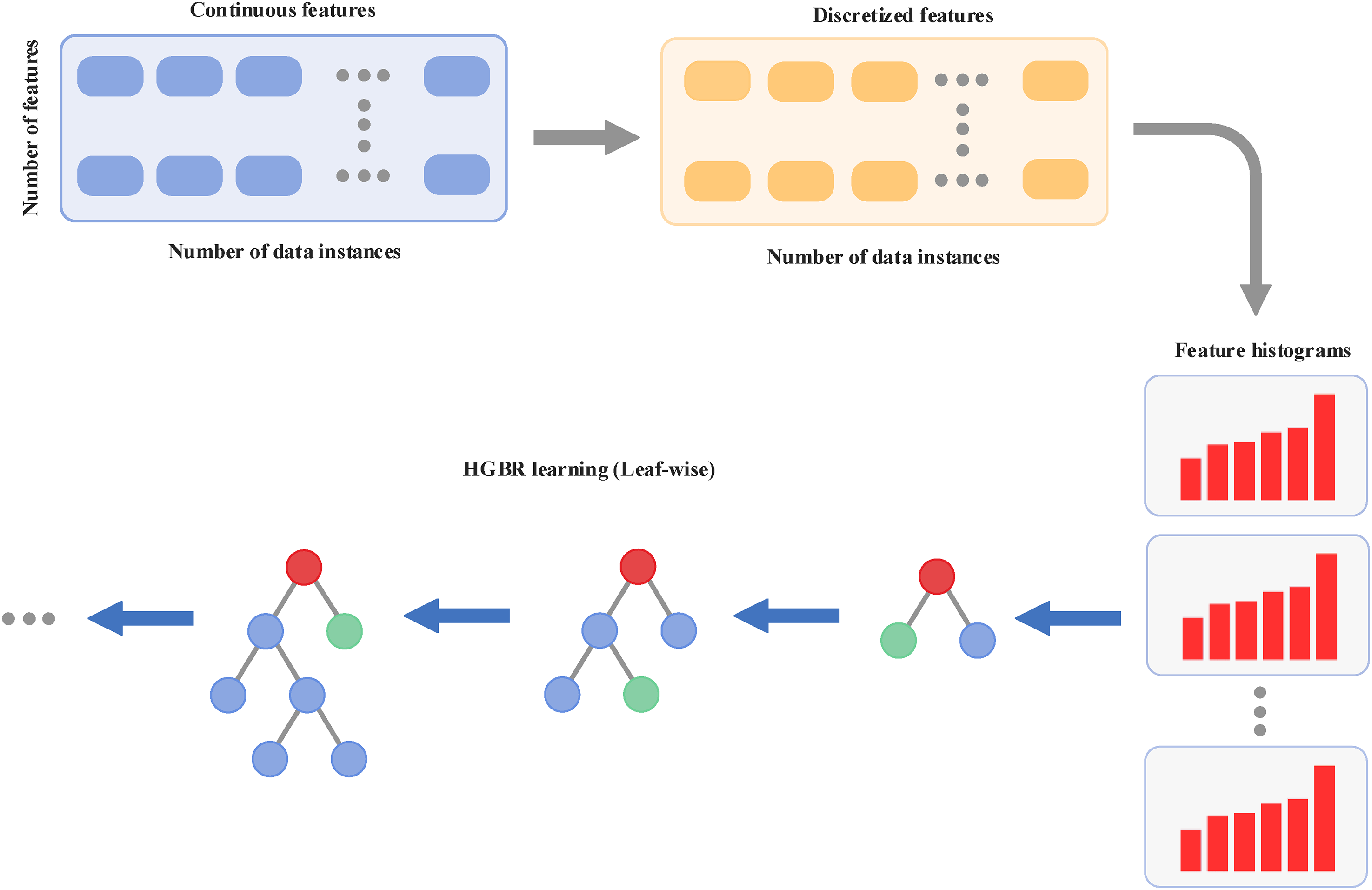
The histogram-based approach structure.

Decomposition method

The VMD model or variable mode decomposition is basically a technique of data decomposing. VMD in signal processing utilizes signals of time series with intrinsic IMF, inherent functions set. Each of these IMFs is expected to characterize only one underlying the original signal detailed oscillatory mode or portion.⁶² The VMD method plays a key role in breaking down complex signals into small interpretable signals. The use of VMD was found to simplify the understanding and interpretation of difficult and complex signals, and, ultimately, more accurate predictions could be provided through this analysis method.⁶³

The advantages that VMD has over other methods are that VMD is a data-driven method and requires no prior knowledge and assumptions. VMD can help in predicting solar radiation by analyzing and then identifying and characterizing the patterns of solar radiation. This decomposition technique will be a very useful signal analyzing tool and thereafter for solar radiation prediction. An important point to note is that VMD can be influenced by various factors, some of which are environmental characteristics and solar radiation data.⁶⁴ On begin, the Hilbert transform is applied to each IMF to produce the one-sided spectra. In the second step, the IMF spectrum is transferred to the baseline area by combining it with a measure adjusted to the predicted center frequencies. Furthermore, the range of each IMF is determined utilizing the demodulated signal's Normal smoothness, that is, the square of the gradients L2 parameter. After the main signal was decomposed into several smaller signals using the VMD method, several IMFs were provided. Subsequently, after each IMF was predicted, its estimated bandwidth was summed. 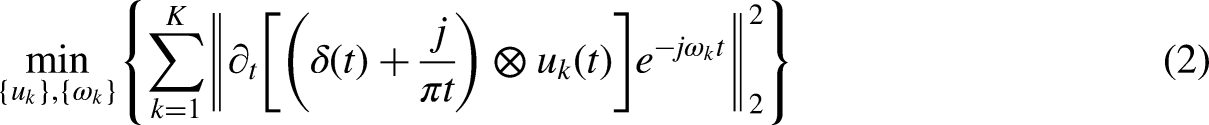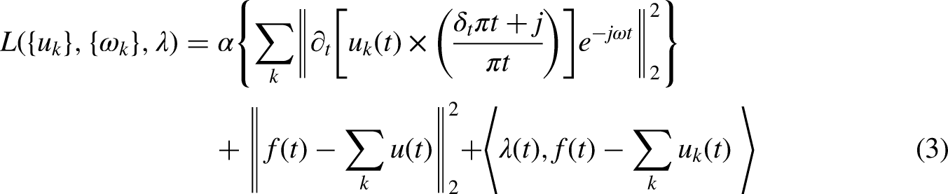In addition, the accumulation of each of the IMFs must be with the input signal $f (t)$ which has a limit. The restricted variational issue is therefore provided as follows:

min_{{u_{k}}, {ω_{k}}} {\sum_{k = 1}^{K} {‖ \partial_{t} [(δ (t) + \frac{j}{π t}) \otimes u_{k} (t)] e^{- j ω_{k} t} ‖}_{2}^{2}}

(2)

Where

{u_{k}}

and

{ω_{k}}

represent the modal element and center frequency ranges, correspondingly. The addition of the cubic punishment and Lagrange multiplier converts the restricted issue to the following unrestrained form:

L ({u_{k}}, {ω_{k}}, λ) = α {\sum_{k} {‖ \partial_{t} [u_{k} (t) \times (\frac{δ_{t} π t + j}{π t})] e^{- j ω t} ‖}_{2}^{2}} + {‖ f (t) - \sum_{k} u (t) ‖}_{2}^{2} + ⟨ λ (t), f (t) - \sum_{k} u_{k} (t) ⟩

(3)

The combination of the quantitative penalization and Lagrangian multipliers gives the benefits of the quadratic penalty's superior convergence skills and the rapid implementation of the constraint by the Lagrangian multiplier. The alternate directions technique of multiplies can be used to solve the equation (3). The two main stages of equation (3) are as follows:

u_k minimization

{\hat{u}}_{k}^{n + 1} (ω) = \frac{\hat{f} (ω) - \sum_{i \neq k} \hat{u} (ω) + (\hat{λ} (ω) / 2)}{1 + 2 α {(ω - ω_{k})}^{2}}

(4)

$ω_{k}$ minimization

ω_{k}^{n + 1} = \frac{\int_{0}^{\infty} ω {| {\hat{u}}_{k} (ω) |}^{2} d ω}{\int_{0}^{\infty} {| {\hat{u}}_{k} (ω) |}^{2} d ω}

(5)

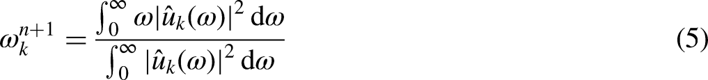
In which n is the total amount of iterations, and the Fourier transform of $λ (ω), u_{k}^{n + 1}, f (ω), u_{i} (ω)$ are represented by $\hat{λ} (ω), {\hat{u}}_{k}^{n + 1}, \hat{f} (ω), {\hat{u}}_{i} (ω)$ , respectively.

Sample entropy

By applying decomposition techniques, a specific time series can be separated into multiple modes. When the algorithm is applied directly, the computational complexity of the forecasting method increases. Taking into account the disaggregated and fragmented components, the SE technique selects and reconstructs patterns to reduce the required computational effort, enabling the analysis of the detail level of the separated elements. Higher SE values indicate stronger autocorrelation, while lower SE values suggest weaker autocorrelation. The following terms can be used to explain the operation of the SE technique.^65,66

Step 1: The following is the definition of the reported time period F with N sample items⁶⁶:

f (1), f (2), f (3), \dots, f (N)

(6)

Step 2: The aforementioned formula can be expressed in m-dimensions as follows:

S_{m} (i) = [f (i), f (i + 1), f (i + 2), \dots, f (i + m - 1)]

(7)

Step 3: Determine and calculate the distances that existed between $F_{i} (i) and F_{m} (j) ([F_{m} (i), F_{m} (j)])$ in the form of ⁶⁶:

d [f_{m} (i)], F_{m} (j) = \max_{k = 0, m - 1} (| u (i + k) - u (j + k) |)

(8)

Step 4: Compute the following $B^{m} (i)$ number utilizing a mean of $B_{i}^{m} (r)$ as:

B^{m} (r) = \frac{\sum_{i = 1}^{N - m + 1} B_{i}^{m} (r)}{N - m + 1}

(9)

$B_{i}$ stands for potential vectors, while $r$ indicates the likelihood for m endpoints within the same tolerance.

Step 5: After repeating steps (2) through (4), get $B^{m + 1} (r)$ as follows⁶⁵:

SE (m, r) = \underset{N \to \infty}{l} [- \ln \frac{B^{m + 1} (r)}{B^{m} (r)}]

(10)

Step 6: The formula above becomes the following when N is assumed to be finite⁶⁵:

SE (m, r, N) = \underset{N \to \infty}{l} [- \ln \frac{B^{m + 1} (r)}{B^{m} (r)}]

(11)

Where r denotes the requirement limit and m represents the way it embeds dimension.

Biogeography-based optimization

Biogeography is the study of the spatial distribution of biological organisms. The development and formulation of mathematical equations governing the dispersal of organisms began in the 1960s.⁶⁷ The concept of nature serving as a source of inspiration for human knowledge has led to the creation of an adaptive algorithm and metaheuristic known as BBO. This method draws upon biogeographic principles such as speciation (the formation of new species), species movement between islands, and species extinction. Initially proposed by Dan Simon in 2008,⁶⁸ BBO utilizes a mathematical framework to model species movement across habitats, characterized by emigration from less favorable habitats and immigration into more suitable ones.

The suitability of habitats is quantified and stored as the habitat suitability index, which is determined by the objective function of the optimization problem being addressed. As one of the most well-known evolutionary algorithms (EAs), BBO optimizes a function by repeatedly and randomly improving the best solutions based on a defined quality or fitness function.⁶⁸ Figure 6 provides a visual representation of the structure of BBO. Figure 7 illustrates the general flowchart of the BBO method, outlining the necessary steps to achieve the optimal solution.

Figure 6.

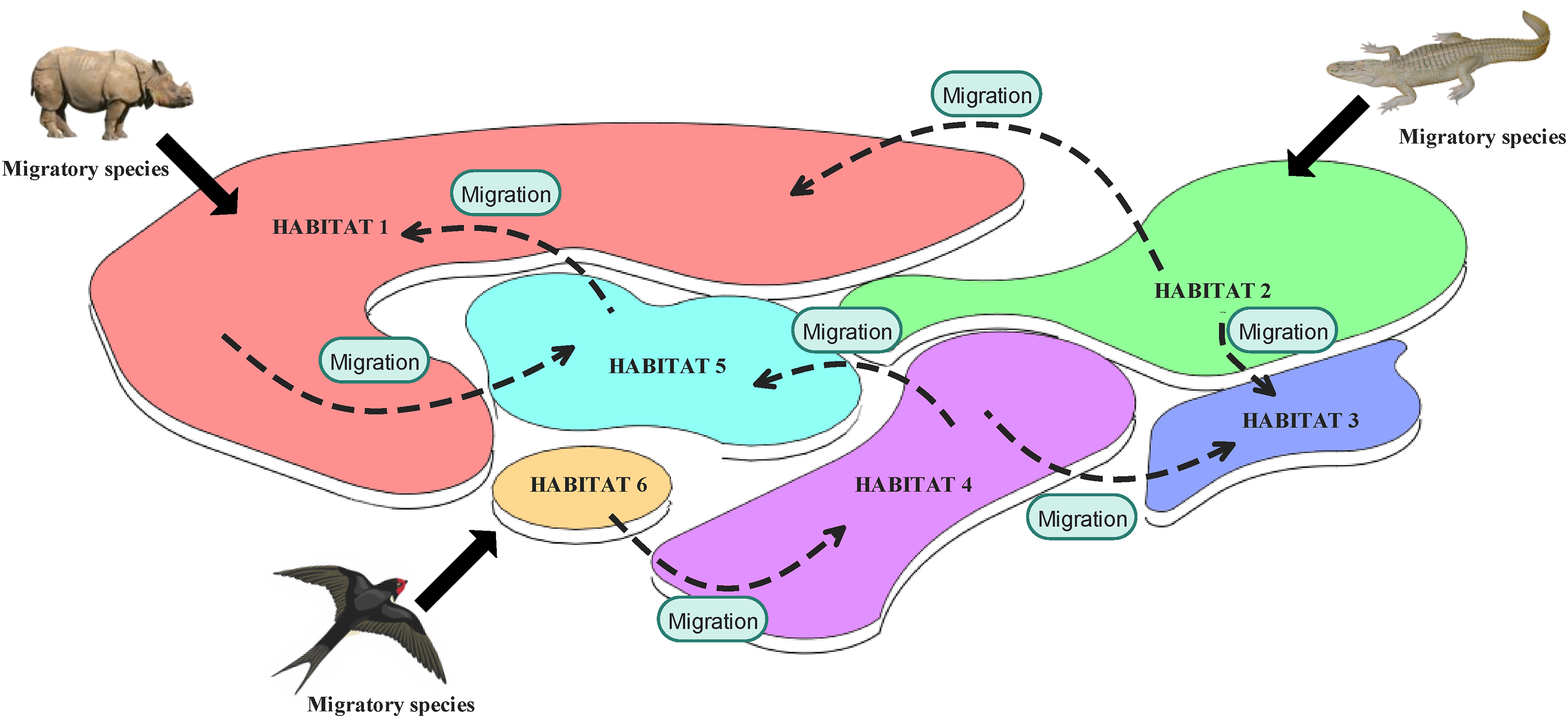
An illustration of biogeography-based optimization.

Figure 7.

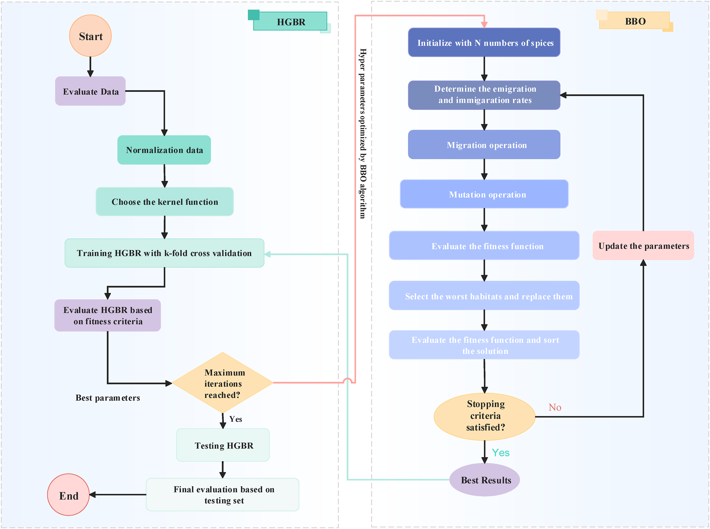
Flowchart of DNI prediction based on BBO-HGBR.

Evaluation metrics

To evaluate the forecasting performance of the two established models, this study employed several key metrics, including root mean square error (RMSE), mean absolute error (MAE), mean absolute percentage error (MAPE), and the coefficient of determination (R²).⁶⁰ Among these, R² is a commonly used metric for assessing the effectiveness of regression models.⁶⁹ It provides valuable insight into how well the model's independent variables (predictors) explain the variation in the dependent variable. The following mathematical formulas describe applied metrics^70,71:

RMSE = \sqrt{\frac{\sum_{i = 1}^{n} {(y_{i} - {\hat{y}}_{i})}^{2}}{n}}

(12)

MAPE = \frac{1}{n} \sum_{i = 1}^{n} | \frac{y_{i} - {\hat{y}}_{i}}{y_{i}} |

(13)

MAE = \frac{\sum_{i = 1}^{n} | y_{i} - {\hat{y}}_{i} |}{n}

(14)

R^{2} = 1 - \frac{\sum_{i = 1}^{n} {(y_{i} - {\hat{y}}_{i})}^{2}}{\sum_{i = 1}^{n} {(y_{i} - \bar{y})}^{2}}

(15)

Applied configuration

The suggested HRS, as shown in Figure 8, offers a scalable and modular design for combining solar power with technologies for hydrogen production and storage. The basic goal of this system's design is to optimize the use of renewable energy sources while preserving operational responsiveness and dependability in the face of fluctuating demand and generation circumstances. PV output scheduling and downstream component operation more precise control. PV arrays produce electricity; irradiance, panel temperature, and environmental losses like dust and aging all affect how well they work. Direct current (DC) electricity produced by the PV modules is sent to both DC and AC loads via a high-efficiency bidirectional inverter. This inverter is essential to the power balance and flexibility of the system because it ensures smooth energy transfer between AC and DC busbars with little loss.

Figure 8.

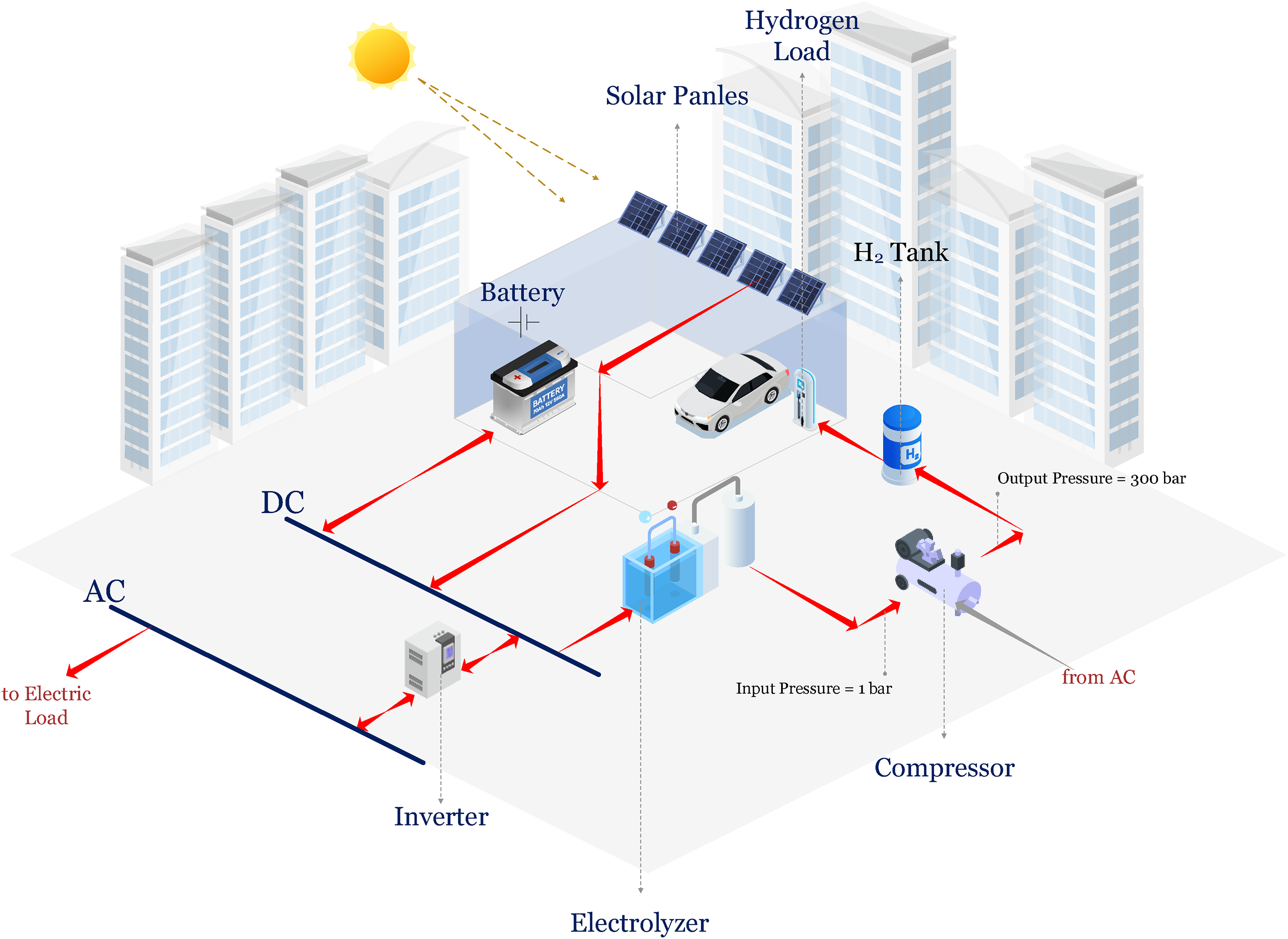
Schematic of the hydrogen refueling station system.

A PEM electrolyzer, which separates water into hydrogen and oxygen, receives the majority of the DC electricity from the PV system. Because of its high hydrogen purity output, quick dynamic response, and compatibility with intermittent renewable inputs, the PEM electrolyzer was selected. Hydrogen is then directed to a compressor, which increases its pressure from atmospheric (∼1 bar) up to standard refueling levels (typically 300 bar depending on vehicle class), making it suitable for storage in a low-pressure hydrogen tank (is approximately 68.75 m³, which corresponds to a spherical vessel with a radius of approximately 2.5 m). The average refueling time per vehicle is designed to fall within 3–5 minutes, subject to tank size, refueling protocol, and temperature compensation strategies. The buffer capacity of the central hydrogen tank ensures that demand surges can be met without immediate reliance on electrolyzer operation.

A battery storage subsystem is another component of the system that serves as a temporary buffer to support system startup, smooth power fluctuations, and handle brief discrepancies between component demand and electricity supply. It is essential for preserving voltage stability, safeguarding delicate parts like the electrolyzer, and increasing operational adaptability. A control and energy management unit coordinates the entire system, dynamically regulating energy flows according to current system status and anticipated solar availability. Reducing curtailment, increasing energy efficiency, and optimizing the flow of hydrogen and electricity are all made possible by accurate DNI forecasting, which allows for proactive modifications to component operation. This arrangement allows for the time-shifting of hydrogen use for energy backup or vehicle refueling because the hydrogen tank functions as the main energy storage medium for longer periods of time. Considering the tank capacities, efficiency, and average range of different commercial FCEVs, the system has been sized to satisfy their refueling needs. From solar generation and forecasting to conversion, buffering, and refueling, this integrated workflow creates a comprehensive and repeatable model for green hydrogen production suited to transportation requirements.

Mathematical modeling

Photovoltaic

Solar panels are devices that transform solar radiation into electrical energy. The output power of a solar panel is influenced by many elements, namely irradiance levels, air temperature, and different losses that diminish panel efficiency.⁷² Panel losses include losses in wiring, panel deterioration, and losses attributable to dust, snow, and debris on the panel surface.⁷³ The output power of a solar array is determined by equation (16).⁷⁴

P_{PV} = Y_{PV} f_{PV} (\frac{{\bar{G}}_{T}}{{\bar{G}}_{T, STC}}) [1 + α_{P} (T_{C} - T_{C, STC})]

(16)

In this context, $Y_{PV}$ denotes the nominal power of the photovoltaic array in kW; $f_{PV}$ represents the derating factor expressed as a percentage; ${\bar{G}}_{T}$ and ${\bar{G}}_{T, STC}$ indicate the instantaneous irradiance $(kW / m^{2})$ and the irradiance under standard test conditions ( $1 kW / m^{2}$ ) on the solar panel's surface, respectively; $α_{P}$ is the temperature coefficient that quantifies the adverse effect of rising surface temperature on the PV array's output power in $% / \circ C$ ; $T_{C}$ signifies the surface temperature of the panel in degrees Celsius, while $T_{C, STC}$ refers to the surface temperature under standard test conditions, which is set at $25 \circ C$ .⁷⁵

The output power of solar arrays is in DC, hence the efficiency of the DC–AC inverter $(η_{inv})$ influences the power provided to the electrical load $(P_{inv, out})$ . The influence of inverter efficiency is articulated in the following equation⁷⁵:

P_{inv, out} = η_{inv} \cdot P_{PV}

(17)

This study discusses the use of SunPower E20-327 PV panels, which have a rated capacity of 0.327 kW.

Electrolyzer

The electrolyzer produces hydrogen by electrolysis with electrical energy. Electrolysis is the method of using electricity to decompose water into hydrogen and oxygen.⁷⁶ PEM water electrolyzers are preferred over alkaline water electrolyzers due to their superior efficiency, extended lifetime, enhanced adaptability, and simpler design.^77,78 The chemical processes taking place at the anode and cathode are shown in equations (18) and (19), respectively.

2 H_{2} O \to O_{2} + 4 H^{+} + 4 e^{-}

(18)

4 H^{+} + 4 e^{-} \to 2 H_{2}

(19)

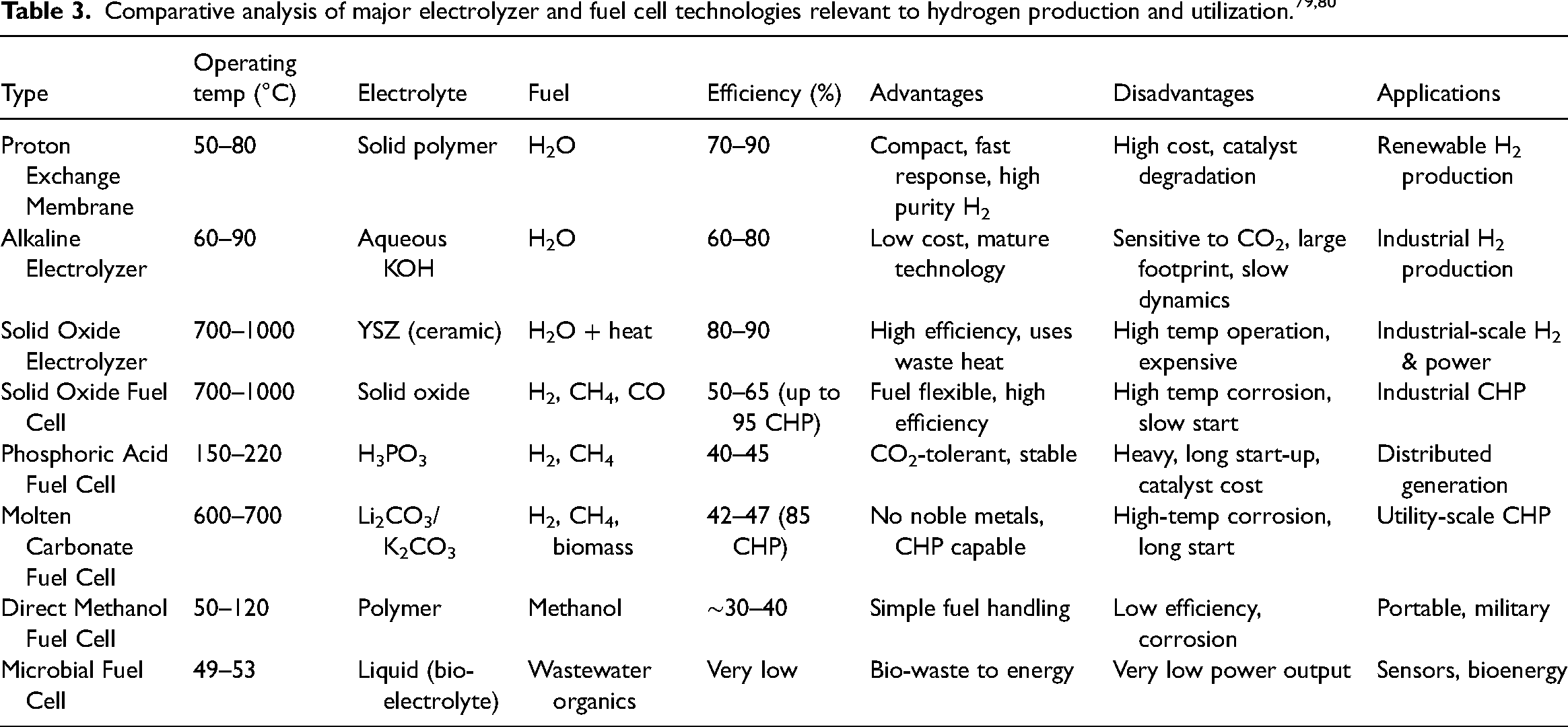
A comparison of the main electrolyzer and fuel cell technologies is given in Table 3 to help further explain the reasoning behind the choice of the PEM in this investigation. High hydrogen purity, quick reaction to varying solar input, small size, and compatibility with renewable energy sources are some of the main benefits of the PEM. For solar-powered hydrogen production systems, like the one created in this study for the Jiangsu hydrogen refueling station, these features make it particularly efficient.

Table 3.

Comparative analysis of major electrolyzer and fuel cell technologies relevant to hydrogen production and utilization.^79,80

Type	Operating temp (°C)	Electrolyte	Fuel	Efficiency (%)	Advantages	Disadvantages	Applications
Proton Exchange Membrane	50–80	Solid polymer	H₂O	70–90	Compact, fast response, high purity H₂	High cost, catalyst degradation	Renewable H₂ production
Alkaline Electrolyzer	60–90	Aqueous KOH	H₂O	60–80	Low cost, mature technology	Sensitive to CO₂, large footprint, slow dynamics	Industrial H₂ production
Solid Oxide Electrolyzer	700–1000	YSZ (ceramic)	H₂O + heat	80–90	High efficiency, uses waste heat	High temp operation, expensive	Industrial-scale H₂ & power
Solid Oxide Fuel Cell	700–1000	Solid oxide	H₂, CH₄, CO	50–65 (up to 95 CHP)	Fuel flexible, high efficiency	High temp corrosion, slow start	Industrial CHP
Phosphoric Acid Fuel Cell	150–220	H₃PO₃	H₂, CH₄	40–45	CO₂-tolerant, stable	Heavy, long start-up, catalyst cost	Distributed generation
Molten Carbonate Fuel Cell	600–700	Li₂CO₃/K₂CO₃	H₂, CH₄, biomass	42–47 (85 CHP)	No noble metals, CHP capable	High-temp corrosion, long start	Utility-scale CHP
Direct Methanol Fuel Cell	50–120	Polymer	Methanol	∼30–40	Simple fuel handling	Low efficiency, corrosion	Portable, military
Microbial Fuel Cell	49–53	Liquid (bio- electrolyte)	Wastewater organics	Very low	Bio-waste to energy	Very low power output	Sensors, bioenergy

To verify the accuracy of the developed PEM electrolyzer model, simulation results were compared with experimental data reported by Ioroi et al.⁸¹ Figure 9 presents a side-by-side comparison of cell voltage versus cell density for both the present study and the reference work. The results show consistent alignment across most voltage ranges, with a maximum deviation of 1.64% observed at peak current density. This validation confirms the model's suitability for accurately representing the electrochemical behavior of PEM electrolyzers under various operational conditions.

Figure 9.

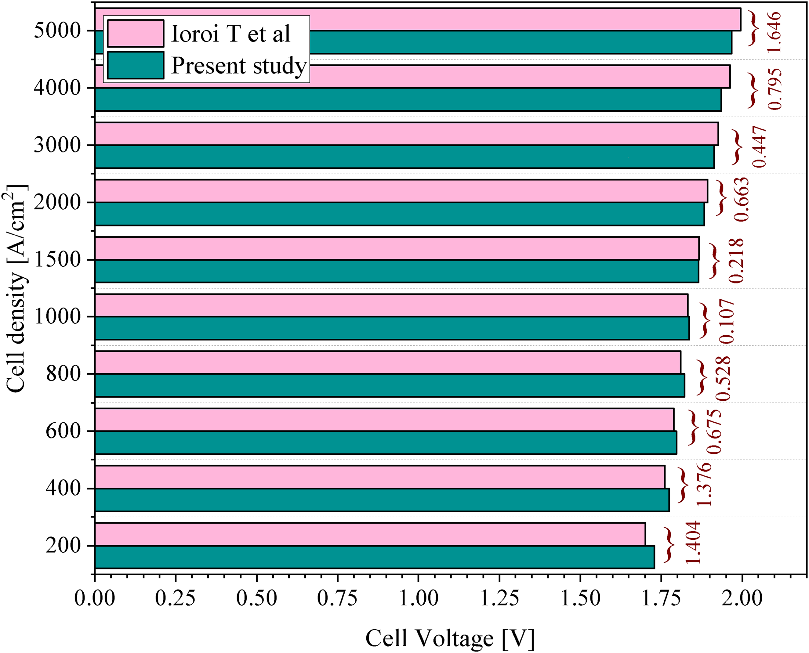
Validation of the PEM electrolyzer model.

Converter

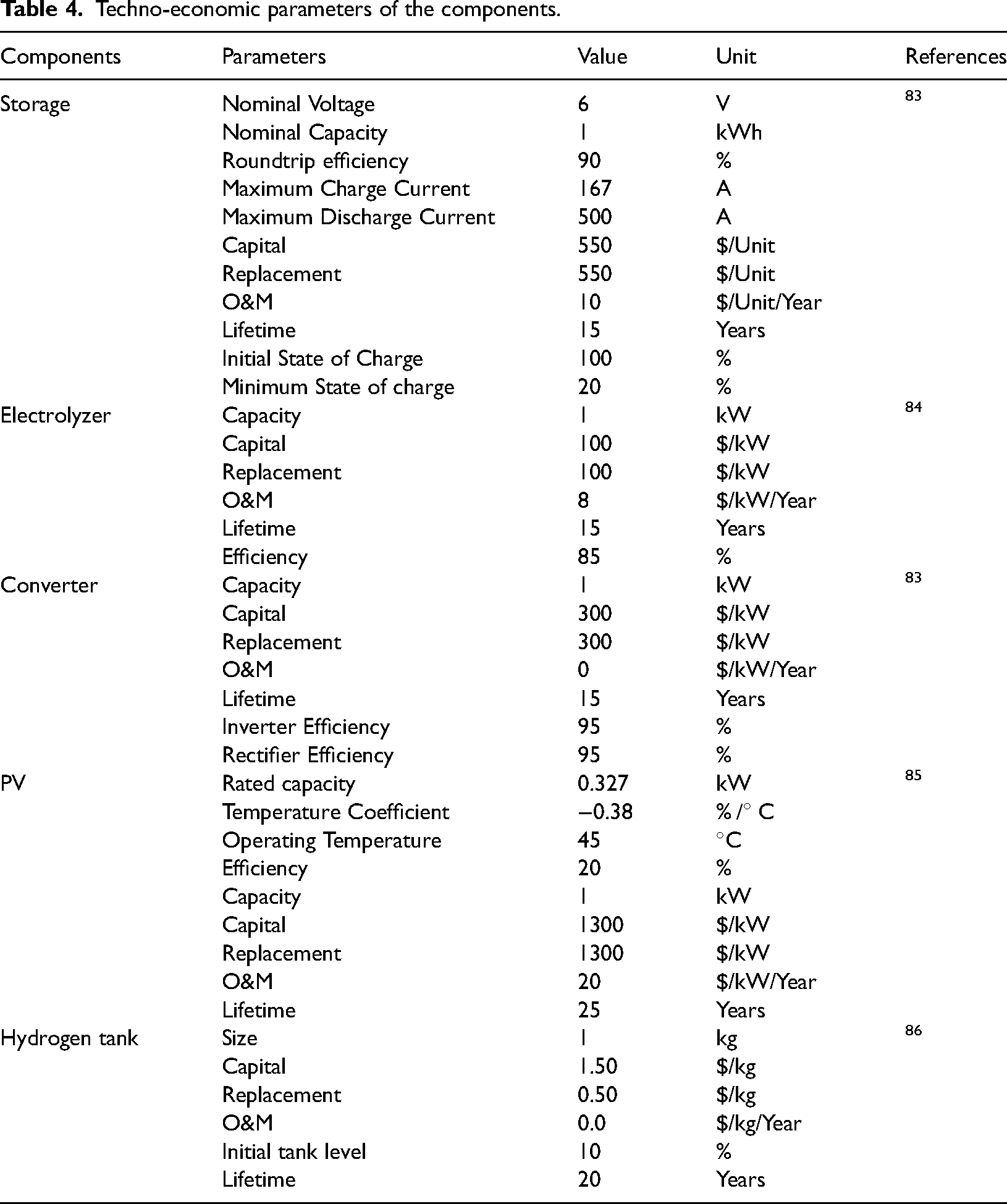
The converter's principal role is to regulate energy transfer between the AC and DC busbars, operating as both an inverter and a rectifier. The converter module's characteristics and specifications are detailed in Table 4. The converter's power rating is dictated by the system's maximum energy demand or supply.⁸² The required rating for the converter in the system is as follows:

P_{conv} = \frac{P_{\max}}{η_{conv}}

(20)

P_{conv}

P_{\max}

, and

η_{conv}

(95%) represent the converter rating, maximum power, and efficiency, respectively.

Table 4.

Techno-economic parameters of the components.

Components	Parameters	Value	Unit	References
Storage	Nominal Voltage	6	V	⁸³
	Nominal Capacity	1	kWh
	Roundtrip efficiency	90	%
	Maximum Charge Current	167	A
	Maximum Discharge Current	500	A
	Capital	550	$/Unit
	Replacement	550	$/Unit
	O&M	10	$/Unit/Year
	Lifetime	15	Years
	Initial State of Charge	100	%
	Minimum State of charge	20	%
Electrolyzer	Capacity	1	kW	⁸⁴
	Capital	100	$/kW
	Replacement	100	$/kW
	O&M	8	$/kW/Year
	Lifetime	15	Years
	Efficiency	85	%
Converter	Capacity	1	kW	⁸³
	Capital	300	$/kW
	Replacement	300	$/kW
	O&M	0	$/kW/Year
	Lifetime	15	Years
	Inverter Efficiency	95	%
	Rectifier Efficiency	95	%
PV	Rated capacity	0.327	kW	⁸⁵
	Temperature Coefficient	−0.38	$% / \circ C$
	Operating Temperature	45	$\circ C$
	Efficiency	20	%
	Capacity	1	kW
	Capital	1300	$/kW
	Replacement	1300	$/kW
	O&M	20	$/kW/Year
	Lifetime	25	Years
Hydrogen tank	Size	1	kg	⁸⁶
	Capital	1.50	$/kg
	Replacement	0.50	$/kg
	O&M	0.0	$/kg/Year
	Initial tank level	10	%
	Lifetime	20	Years

Storage

The battery stores electricity chemically, allowing the stored energy to be recharged and utilized for continued functioning as needed. To ensure the lifespan of the battery bank, it is essential to maintain the battery charge within 20%.⁸⁷ This study assumes four battery technologies, with their specifications detailed in Table 4. The below equation illustrates the estimation of battery energy levels.⁸⁸

Q_{battery} = Q_{battery, 0} + \int_{0}^{τ} V_{battery} I_{battery} d t

(21)

Q_{battery, 0}

(kWh) represents the initial battery charge,

V_{battery}

(V) denotes the battery voltage, while

I_{battery}

(A) indicates the battery current. The state of battery charge is denoted by equation (22).

B_{soc} = \frac{Q_{battery}}{Q_{battery, \max}} \times 100 (%)

(22)

Hydrogen tank

The volume of hydrogen produced has practical uses and may be used across several industries, mostly for recharging hydrogen cars. Excess electricity or lack of hydrogen demand results in the storage of hydrogen generated by the electrolyzer in a hydrogen tank. The beginning tank level in this investigation is set at 10% of the tank's capacity, using a standard hydrogen tank. The capacity of the hydrogen tank was assessed within a defined range of 0 to 2000 kg. Table 4 presents the efficiency of the hydrogen tank together with the comprehensive cost estimates.⁸⁶

Hydrogen fuel cell electric vehicles

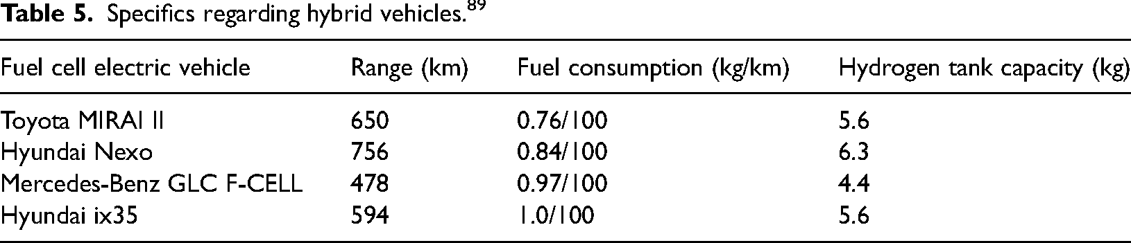
A comparison of performance and requirements was conducted for the various hydrogen cars are illustrated in Table 5. The range, fuel efficiency, and hydrogen tank capacity for chosen FCEVs including Toyota MIRAI II, Hyundai Nexo, Mercedes-Benz GLC F-CELL, and Hyundai ix35 are presented. These specs illustrate the concept of energy demand and storage capacity for the efficient refueling of automobiles. The Hyundai Nexo offers the longest range at 756 km, predicated on an economical fuel consumption of 0.84 kg/100 km and a hydrogen tank capacity of 6.3 kg. In contrast, the Mercedes-Benz GLC F-CELL achieves a shorter distance of merely 478 km, attributed to a higher fuel consumption of 0.97 kg/100 km and a smaller hydrogen tank capacity of 4.4 kg. Consequently, both the Toyota MIRAI II and Hyundai ix35 exhibit commendable performance in this regard, with ranges of 650 km and 594 km, respectively, while their hydrogen consumption rates are correlated with tank capacity. This data supports the need to enhance hydrogen storage and refueling infrastructure, taking into account the diverse energy requirements of these vehicles. Thus, this substantiates the need of developing a scalable hydrogen filling station capable of accommodating various applications for FCEVs.

Table 5.

Specifics regarding hybrid vehicles.⁸⁹

Fuel cell electric vehicle	Range (km)	Fuel consumption (kg/km)	Hydrogen tank capacity (kg)
Toyota MIRAI II	650	0.76/100	5.6
Hyundai Nexo	756	0.84/100	6.3
Mercedes-Benz GLC F-CELL	478	0.97/100	4.4
Hyundai ix35	594	1.0/100	5.6

Carbon footprints of hydrogen production methods

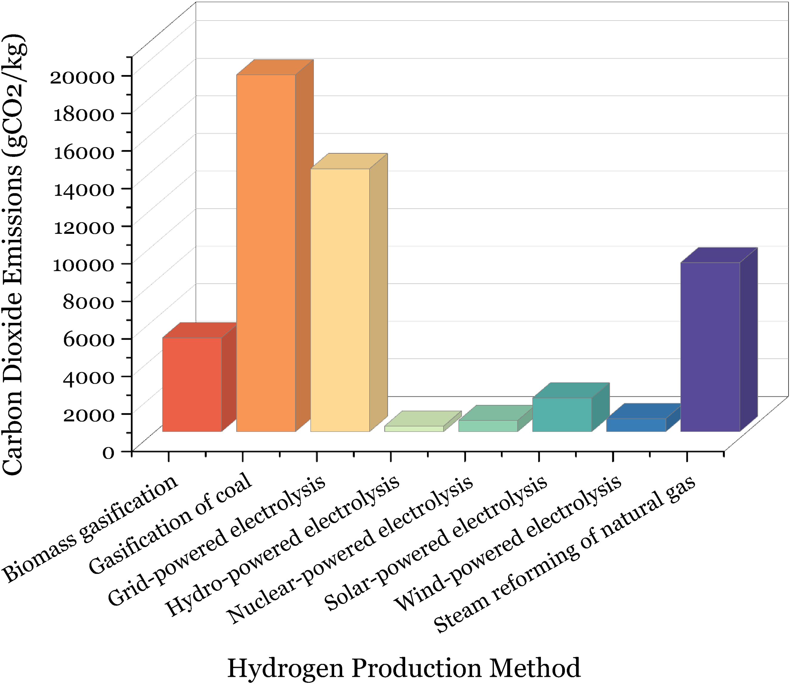
Figure 10 provides a summary of the carbon dioxide emissions associated with different hydrogen generating processes. Biomass gasification emits 5000 units of ${CO}_{2}$ , while coal gasification generates a much greater amount of 19,000 units. Solar-powered electrolysis produces 1800 units of ${CO}_{2}$ , but grid-powered electrolysis generates 14,000 units. The predominant industrial technique, steam reforming of natural gas, generates 9000 units of ${CO}_{2}$ . Solar-powered electrolysis is the most ecologically sustainable method, since it utilizes renewable energy and generates minimum emissions.

Figure 10.

CO₂ emissions associated with various hydrogen production techniques.⁹⁰

Economic criteria

NPC is derived from the assessment of the comprehensive expenditures related to a project, including capital, operational, and maintenance costs. The NPC during the project's duration is computed as^91,92:

NPC = \frac{C_{ann, tot}}{CRF (i, n)}

(23)

C_{ann, tot} = C_{cap} + C_{rep} + C_{O & M} - R_{salv}

(24)

i = \frac{i - f}{1 - f}

(25)

CRF = \frac{i {(1 + i)}^{n}}{{(1 + i)}^{n} - 1}

(26)

where

C_{ann, tot}

($/year) denotes the total yearly cost, CRF signifies the capital recovery factor, i represents the annual interest rate (%), and n indicates the lifespan of the hybrid system.

C_{ann, tot}

C_{rep}

C_{O & M}

, and

R_{salv}

denote the total yearly cost, replacement cost, total operating and maintenance cost, and salvage value, respectively, while the nominal interest rate is represented by i and the annual inflation rate by f.

The LCOH is used to evaluate the feasibility of an energy system. It denotes the mean expense of generating and distributing a unit of hydrogen during the system's operational duration, including for capital expenditures, operational and maintenance costs, and the system's lifespan. The calculation involves dividing the entire yearly cost by the annual hydrogen output as shown in⁹³:

LCOH = \frac{C_{ann, tot}}{M_{H_{2}}}

(27)

In this setting, LCOH denotes the levelized cost of hydrogen ($/kg), whereas

M_{H_{2}}

signifies the yearly hydrogen production (kg/year).

Study framework

The proposed model integrates advanced data processing techniques and renewable energy optimization to create a comprehensive framework for efficient hydrogen production and storage. This study combines machine learning methodologies with sustainable energy solutions to address the challenges of clean energy management. The workflow of the model is detailed step-by-step in Figure 11. The process begins with data preprocessing and correlation analysis, where raw data is collected, refined, and analyzed to identify significant correlations with DNI. Irrelevant data points are removed to finalize a robust dataset suitable for further analysis. The prepared dataset is further divided into four seasonal subsets, namely Spring, Summer, Autumn, and Winter. Further, each subset has been split into training and testing datasets comprising 80% for training and 20% for testing to effectively gauge the predictive performance of the model. First of all, benchmark models are compared by using the prepared dataset in order to find the best model among the three machine learning approaches taken for comparison. Once the optimal model is identified, it undergoes hyperparameter optimization to enhance its performance. Following optimization, the prediction accuracy of the model is further improved by utilizing the decomposed dataset and clustering processes. In the case of VMD, seasonal data is decomposed into small and manageable signal components for further analysis of signals in detail. Further, the process goes ahead to the clustering and consolidation of the signals after decomposition. The SE method will be applied in the grouping of such signals into classes like High, Medium, Low, and Residual classes for a focused analysis of certain behaviors of these signals. The optimized BBO-HGBR network predicts the clustered signals, and the resulting outputs are aggregated to produce the final prediction outcomes. These predictions are then seamlessly integrated into the hydrogen refueling station framework, ensuring efficient and reliable energy management. The station is powered by a PV array, which converts solar energy into DC electricity. This energy is processed through an inverter to supply AC to system components. Hydrogen is produced in the PEM electrolysis water. The excess energies from the photovoltaic are either stored at short-term fluctuations or converted into hydrogen for long-period storage in the battery unit. Hydrogen generated from each and every producing unit is passed through high-pressure tanks for high-capacity purposes, which eventually work as a suitable energy source that can be either employed for vehicle fueling or is used as backup during periods with a lack of sufficient renewable energy conversion. The integration of advanced data processing, renewable energy optimization, and scalable hydrogen refueling infrastructure demonstrates a sustainable and efficient approach to meeting clean energy demands. The system ensures flexibility, and maximum utilization of renewable resources, contributing to the growing adoption of hydrogen as a clean energy solution.

Figure 11.

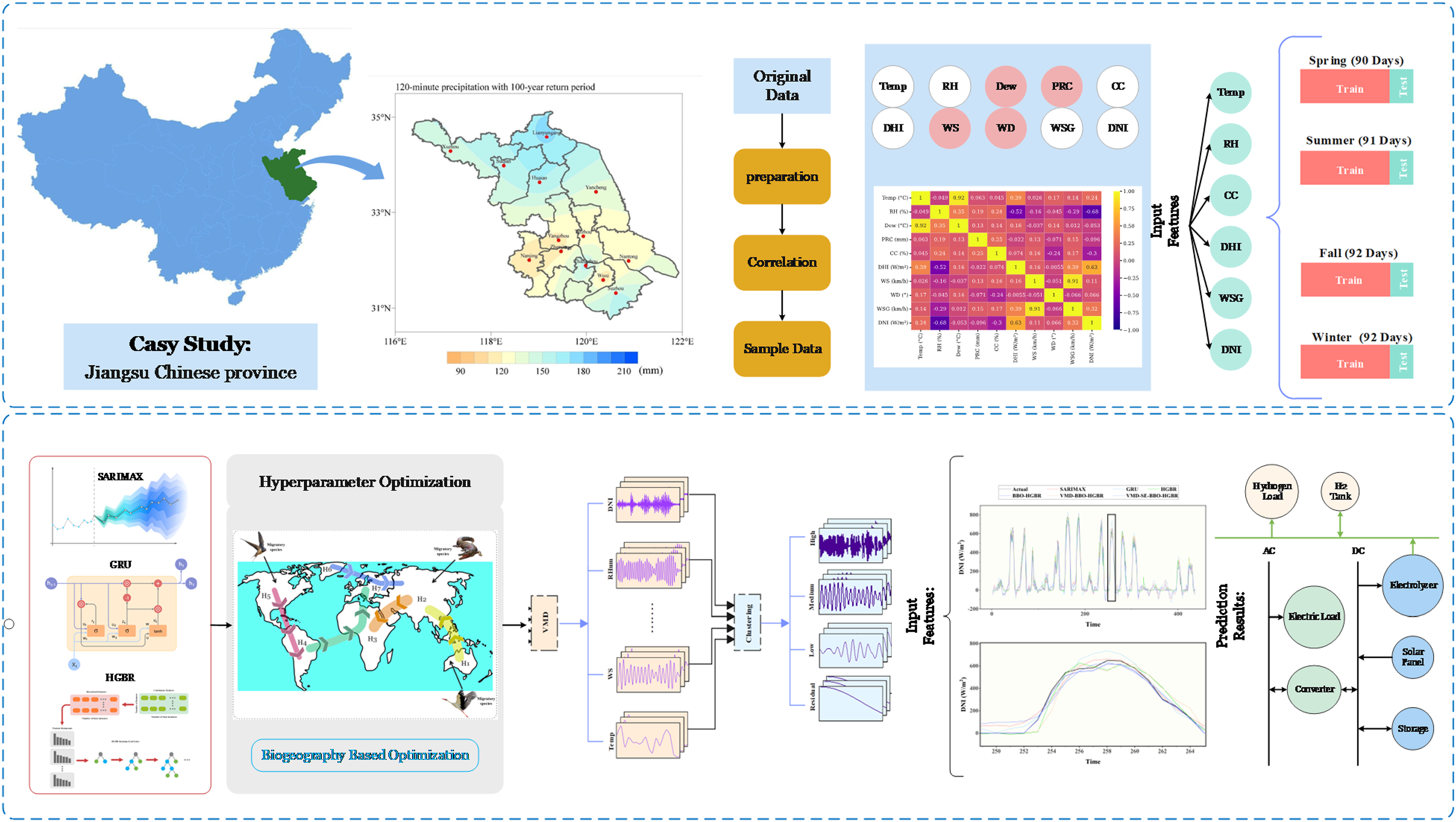
A step-by-step flowchart outlining the overall process of the proposed model.

Results and discussion

Data decomposition

The VMD method is an important approach in this work, decomposing the complex time-series data into simpler, more interpretable components. This technique is especially suitable for capturing seasonal variability in DNI, which is one of the most important variables in renewable energy forecasting. The VMD technique helps in the detailed analysis of the signal by decomposing the DNI signal into IMFs and a residual component, which will increase the accuracy of the predictive models.^94,95 Figure 12 depicts the implementation of the VMD method on the DNI time-series data, categorized by season comprising Spring, Summer, Autumn, and Winter. This decomposition is essential for converting complicated, nonlinear, and non-stationary data into separate components that facilitate analysis. The VMD allows for the decomposition of the DNI signal into seven IMFs and a residual component, in descending frequency and ascending wavelength order for Spring season. The decomposition done here forms the basis for subsequent signal clustering and predictive modeling within the framework of the study. This is supported by the seasonal decomposition, which supports the two major phases of the study. First, it allows the detailed analysis of the signal and its clustering by splitting the signals into high, medium, low, and residual groups, which can enable the focused study of different seasonal behaviors of these signals. Second, the decomposed signals improve predictive accuracy for the optimized BBO-HGBR network, leading to better predictions of both DNI and renewable energy output. This enables the research to discern seasonal fluctuations, indicating that conditions may alter with each season, while also augmenting the robustness of the forecast model. The higher-order IMFs indicate rapid and transient variations resulting from sporadic meteorological phenomena, such as cloud cover, in the spring season. The mid-range IMFs signify medium-term fluctuations, exhibiting semi-daily oscillations in meteorological circumstances. The residual component establishes a consistent baseline trend that aligns with the overall solar radiation pattern for Spring as demonstrated in Figure 12(a). This breakdown pertains to frequent fluctuations in solar energy throughout this season, necessitating good clustering and prediction techniques. During summer, the higher-order IMFs are characterized by less short-term swings due to steady meteorological conditions prevalent in this season demonstrated in Figure 12(b). Mid-range IMFs, namely IMF3 to IMF6, predominate with periodic fluctuations in diurnal cycles. This residual component exhibits elevated and steady baseline solar radiation in summer, making the season particularly dependable for solar energy generation owing to its stability and reduced short-term variability. The accurate prediction of mid-range IMFs is crucial for generating a precise projection of output energy.

Figure 12.

The results of the data decomposition across different seasons: (a) spring, (b) summer, (c) autumn, and (d) winter.

The higher-order IMFs for Autumn are IMF1–IMF3, indicating active short-term variations and therefore unpredictable weather as the season transitions into winter as presented in Figure 12(c). The mid-range IMFs of IMF4–IMF6 correspond to modest periodic fluctuations, indicative of semi-stable situations. The residual component reveals a diminishing baseline trend corresponding with decreased sun radiation in autumn. This kind of seasonal decomposition makes it an appropriate transitional variation of solar radiation, combining stability with variability in order to give effective energy forecasts. The higher-order IMFs (IMF1–IMF3) indicate a pronounced activity during Winter as outlined in Figure 12(d), signifying frequent short-term fluctuations attributed to gloomy weather, snowfall, or reduced daylight duration. Mid-range IMFs are hardly discernible due to the modest periodic fluctuations throughout this timeframe. The residual component provides a low and constant baseline, indicating less solar radiation. Winter data decomposition illustrates the challenges in predicting caused by significant amplitude, high-frequency noise and a little steady-state baseline trend. High-order IMFs encapsulated short-term changes, mid-range IMFs illustrated medium-term patterns, whilst the residual component represented the baseline trend. These investigations are crucial in enhancing the performance of the BBO-HGBR network, notably in clustering and predictive modeling. It addresses the distinct characteristics of each season, so facilitating accurate energy forecasting, optimizing hydrogen production, and enhancing the sustainable and effective operation of clean energy systems.

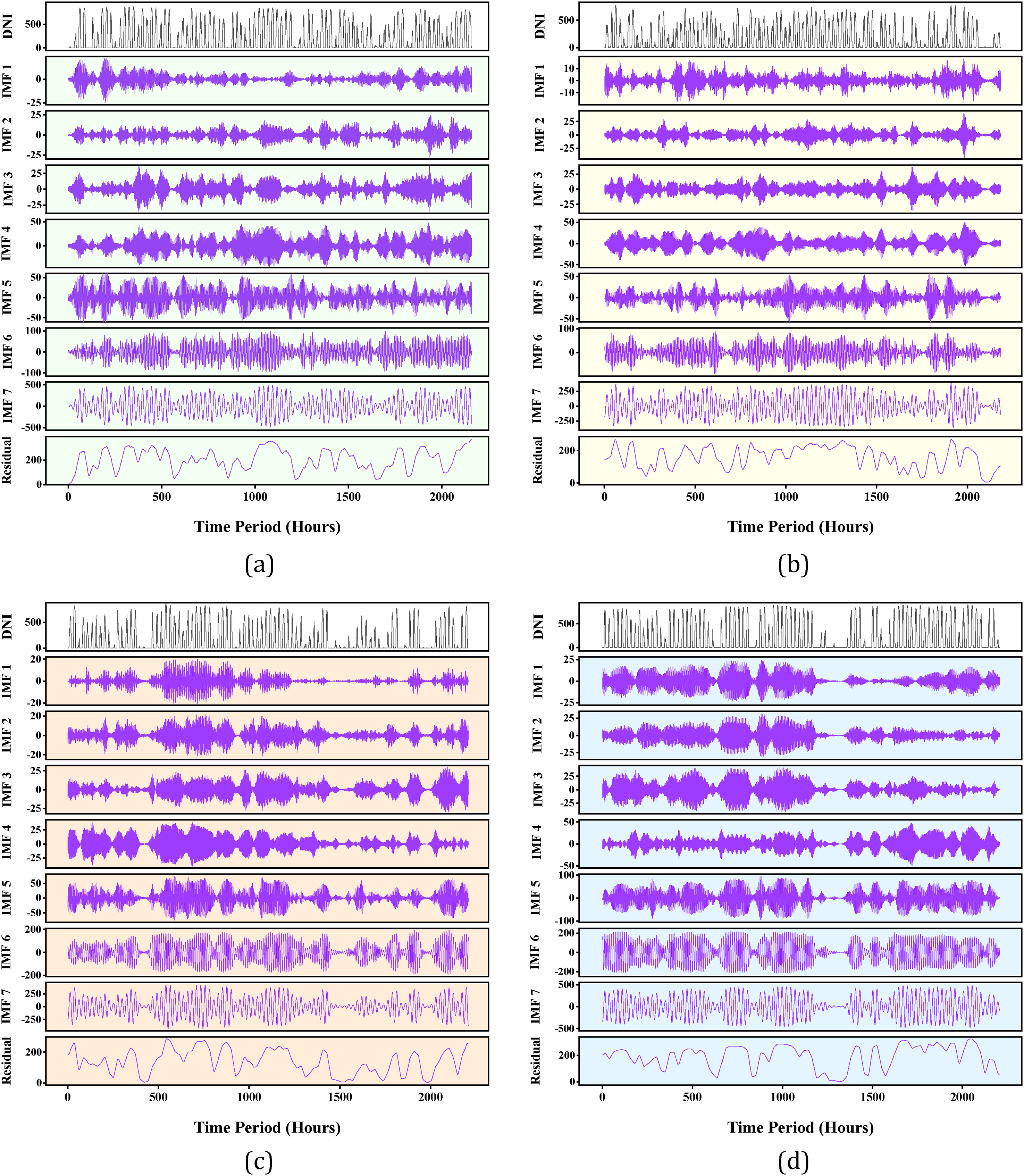
Computation of sample entropy

The computing requirements of the model might markedly escalate if all modal components derived from VMD processing are used. The generation of numerous modes via VMD necessitates the processing of extensive data, hence augmenting both the processing duration and computing complexity. The SE method is used to mitigate the total computing cost associated with this difficulty.⁶⁵ The SE approach categorizes various states based on their corresponding SE values, reducing the need for individual mode analysis and significantly streamlining the computing process.⁹⁶ In this approach, SE values are computed for all created states to measure the complexity of the signal. The SE quantifies the degree of unpredictability or disorder within a signal; elevated SE values indicate a more intricate and less predictable signal, whilst lower SE values denote simpler or more regular signal patterns. Figure 13 shows that the value of SE is directly proportional to signal complexity: the higher the value of SE, the more complex and detailed the signal, while the lower the value of SE, the simpler and more ordered the signal is. The last step is to divide the complexity of the signals into four groups, each of them according to its value of SE, so that the clarity of the features displayed by the analyzed signal is enhanced. The first category, known Residual, encompasses signals with SE values between 0 and 0.25, indicating little complexity. These indications are often consistent and foreseeable. The second group, with low complexity, includes signals with SE values ranging from 0.25 to 1, indicating signals that exhibit considerable fluctuation while remaining relatively simple. The third group, with medium complexity, encompasses signals with SE values between 1 and 1.5, indicating patterns that are more intricate and less predictable. The high complexity category encompasses signals with SE values over 1.5, indicative of very complex signals marked by significant unpredictability and disorder. The complexity of the signals is included into this categorization, facilitating the assessment of different degrees of signal intricacy and optimizing the computer resources needed for further analysis, hence alleviating the processing burden.

Figure 13.

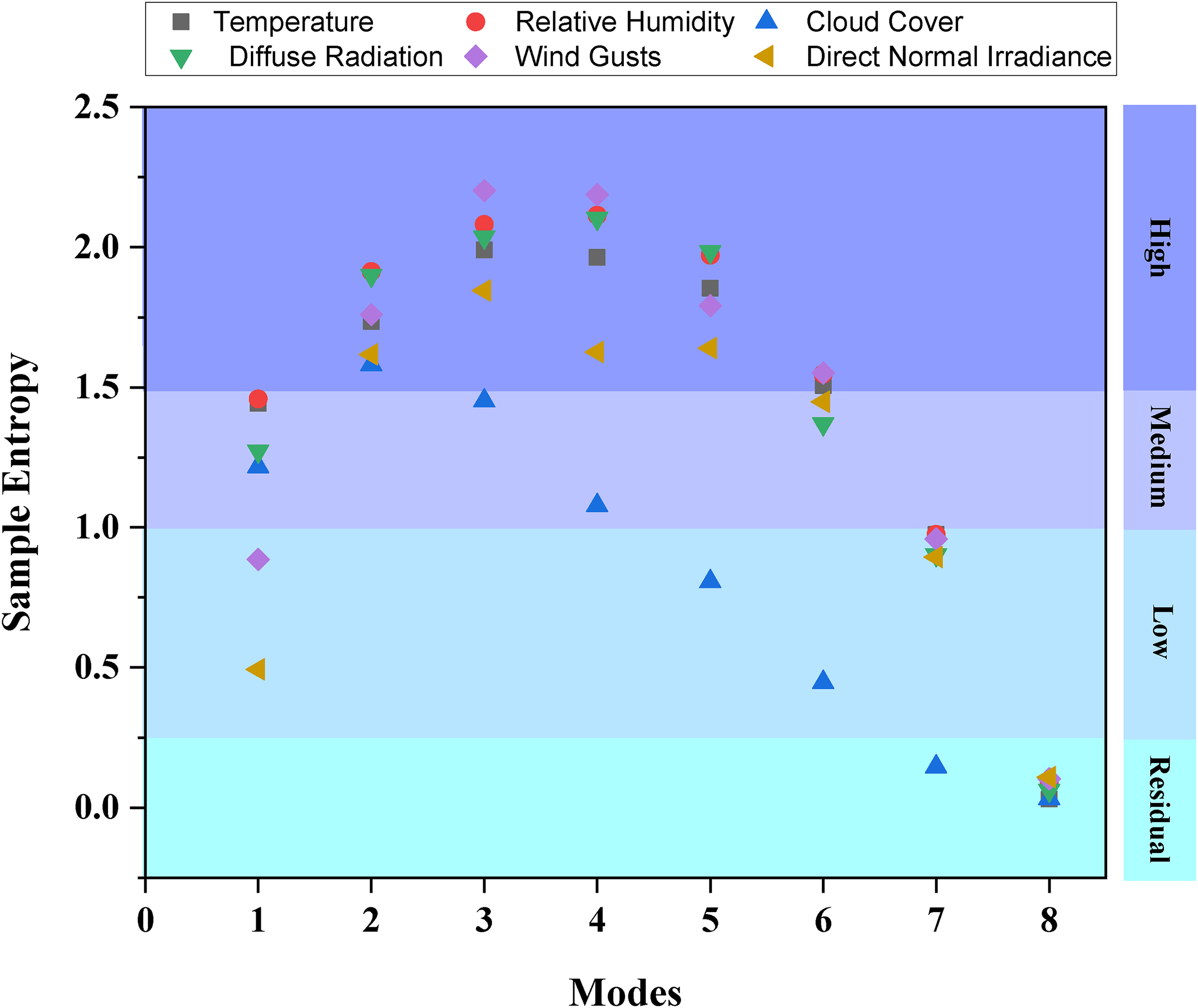
Calculation of sample entropy for VMD-derived decomposed.

Hyperparameter optimization

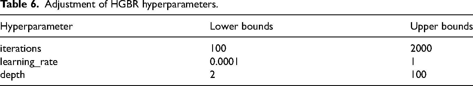
Perfect operation of models depends on exact specification of hyperparameters. Setting the ideal hyperparameter settings will help to raise processing model correctness. One may discover the ideal hyperparameters by means of manual or automated optimization.⁹⁷ The manual optimization approach selects hyperparameter values through try and error. During this time-consuming procedure, it is possible that the poorest hyperparameter values can be applied. It necessitates extensive knowledge of the parameters as well as competence in the relevant sector. Furthermore, the procedure might be time-consuming and not always dependable. The automated optimization method, on the other hand, is more successful since it employs optimizers to automatically determine the best hyperparameters.⁹⁸ This approach benefits from using algorithms that can simultaneously maximize many aspects, hence accelerating and improving the process. Moreover, it can manage complex models more skillfully than the hand-based optimization approach. When the parameters are difficult to understand or too numerous to handle by hand, the automated procedure comes in handy. While human optimization can be ideal in some certain situations, auto-optimization is more effective, reliable, and accurate for finding the best hyperparameters. In the current study, the BBO optimizer was used for the optimization of the hyperparameters of the HGBR model. Optimization of the models required defining the lower and upper bounds of the hyperparameters. The lower and upper boundaries of the hyperparameters are reported in Table 6. These hyper-parameters were then fine-tuned for optimum results using the BBO optimizer and henceforth improving the precision of the HGBR model.

Table 6.

Adjustment of HGBR hyperparameters.

Hyperparameter	Lower bounds	Upper bounds
iterations	100	2000
learning_rate	0.0001	1
depth	2	100

Prediction results

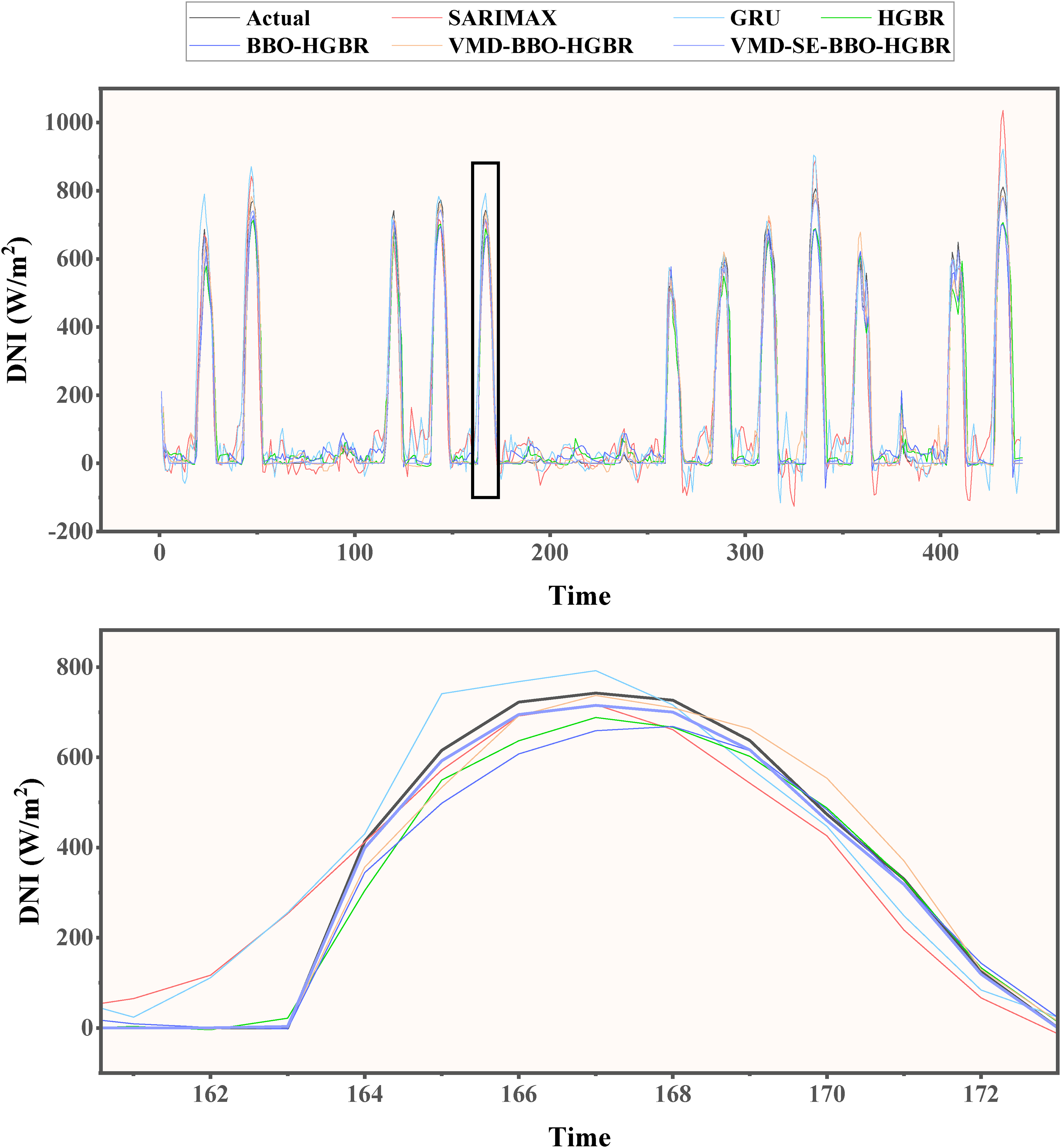
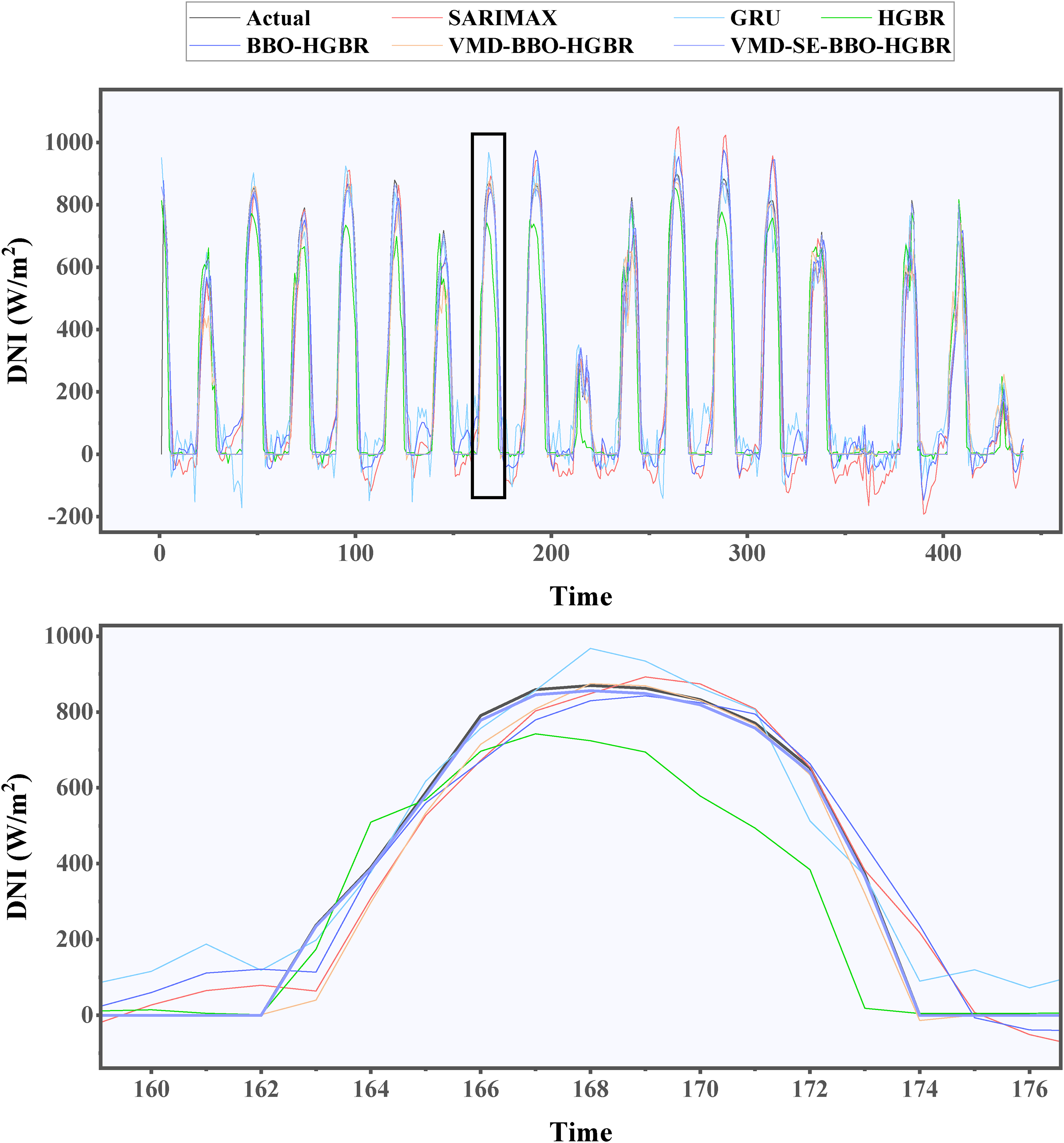
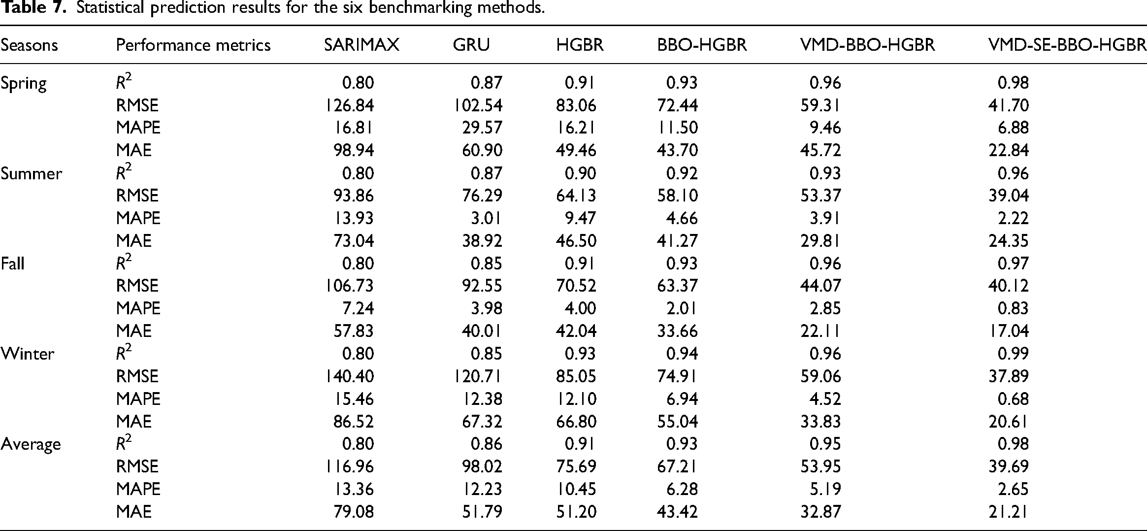
The test data of all four seasons were used to test these models to evaluate their performance in the prediction of DNI. The different performance measures of models, MAE, RMSE, MAPE, and the R², are illustrated in Table 7 and Figure 14. Because of geographical and climatic reasons, solar irradiance shows a seasonal pattern; therefore, the data set is split into separate subsets for Spring, Summer, Autumn, and Winter. The idea is that such a division into seasons can ensure that these models will be tested for their performance across different settings-indeed similar in real-life application scenarios. Among the six proposed models, the performance of VMD-SE-BBO-HGBR was promising in all evaluated metrics. It had an average R² of 0.98, markedly surpassing the other three models assessed comprising the SARIMAX model at 0.80, GRU at 0.86, and HGBR at 0.91. Furthermore, the integration of BBO with VMD enhanced the efficacy of the HGBR model, as shown by the elevated R² values from 0.93 with BBO alone to 0.95 when both VMD and BBO are used in conjunction, resulting in the VMD-BBO-HGBR model. These findings suggest the use of embedding decomposition, clustering, and optimization methods to enhance the prediction efficacy of conventional machine learning models. The lowest RMSE for the optimal model, VMD-SE-BBO-HGBR, fluctuated between 37.89 W/m² and 41.70 W/m² across seasons, yielding an annual average of 39.69 W/m². The findings indicate that the MAPE ranged from 0.68% to 2.65%, with an annual mean of 1.95%. In terms of the yearly average, the MAE was 21.21 W/m², ranging between 20.61 W/m² and 22.84 W/m². These results demonstrate the model's exceptional accuracy in producing projections closely aligned with the values obtained throughout the solar radiation testing phase. Accuracy is key in this respect for renewable energy management systems; even small deviations have the potential to cause huge losses in the efficiency of energy generation and storage. The real-time forecast variations over the seasons corresponding to the different models, such as the SARIMAX, GRU, HGBR, BBO-HGBR, and VMD-BBO-HGBR, are presented in Figures 15–18. The forecasted curves obtained using the VMD-SE-BBO-HGBR model fitted very well with the real solar irradiance data and therefore establish the superiority of the model beyond its competitors. Sophisticated signal decomposition integrated with clustering and optimization approaches captures the key strengths in seasonal fluctuation, thereby allowing VMD-SE-BBO-HGBR to handle the core complexity and nonlinearities inherent in solar irradiance.

Figure 14.

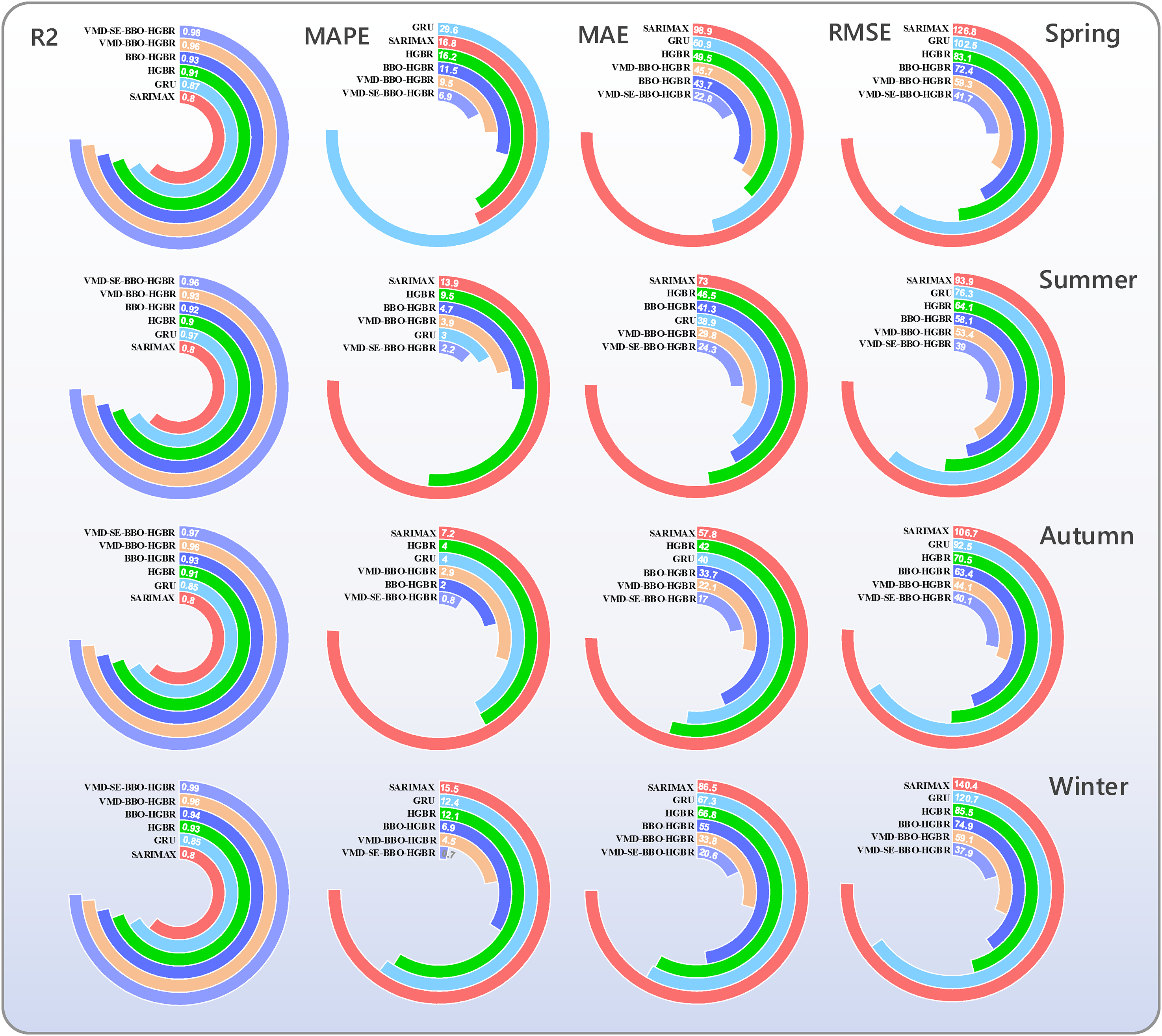
The evaluation values of each model for each season.

Figure 15.

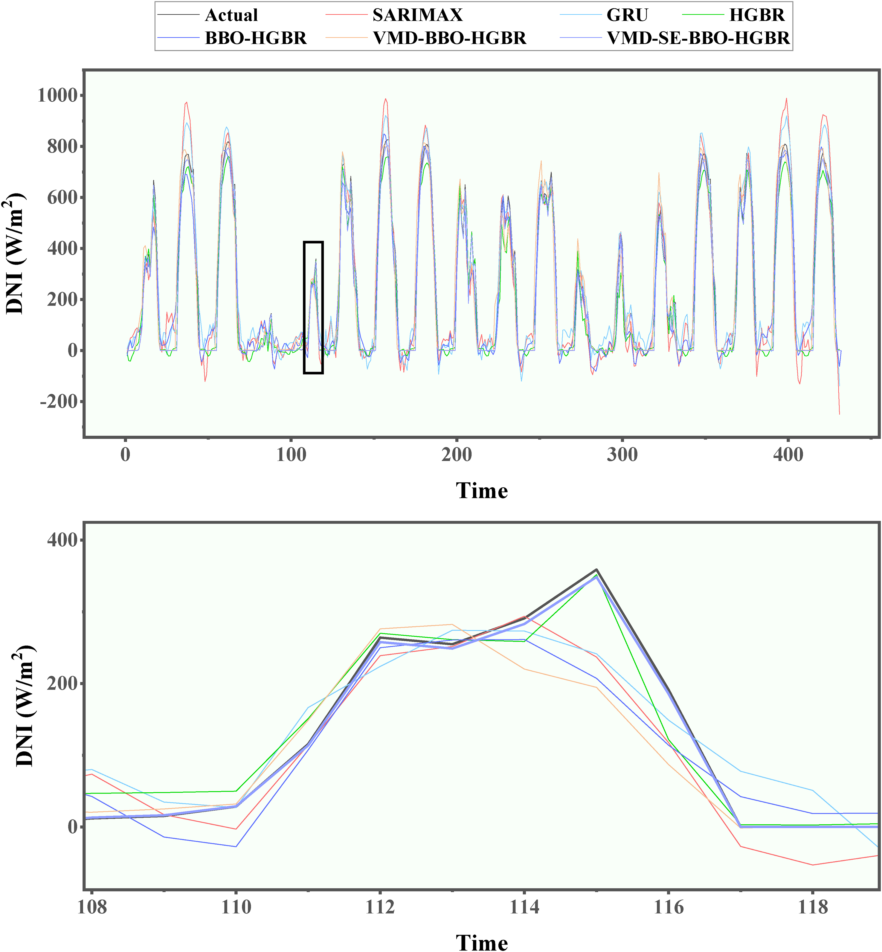
Prediction curves of the generated models during testing for the spring.

Figure 16.

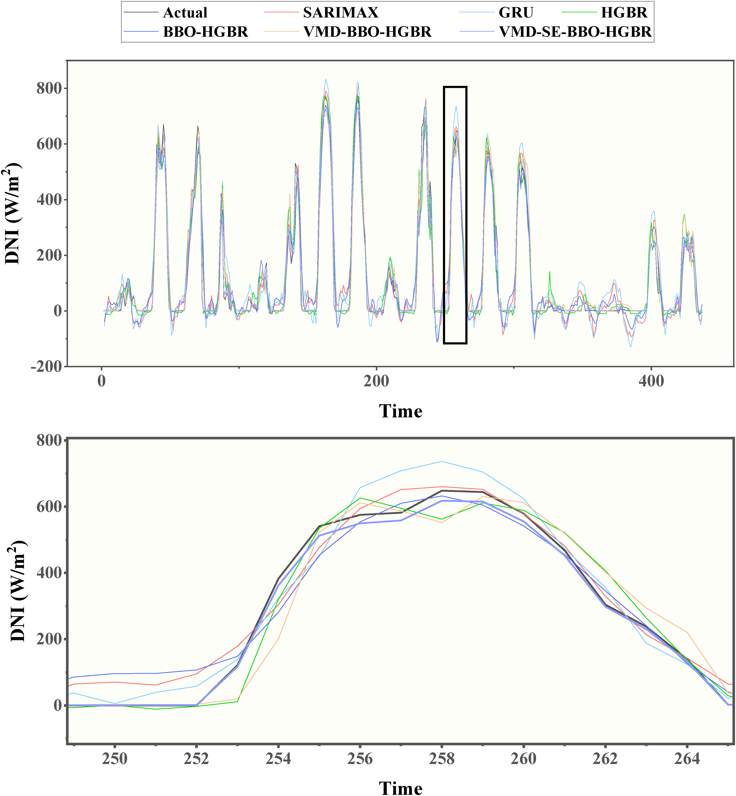
Prediction curves of the generated models during testing for the summer.

Figure 17.

Prediction curves of the generated models during testing for the autumn season.

Figure 18.

Prediction curves of the generated models during testing for the spring season.

Table 7.

Statistical prediction results for the six benchmarking methods.

Seasons	Performance metrics	SARIMAX	GRU	HGBR	BBO-HGBR	VMD-BBO-HGBR	VMD-SE-BBO-HGBR
Spring	R ²	0.80	0.87	0.91	0.93	0.96	0.98
	RMSE	126.84	102.54	83.06	72.44	59.31	41.70
	MAPE	16.81	29.57	16.21	11.50	9.46	6.88
	MAE	98.94	60.90	49.46	43.70	45.72	22.84
Summer	R ²	0.80	0.87	0.90	0.92	0.93	0.96
	RMSE	93.86	76.29	64.13	58.10	53.37	39.04
	MAPE	13.93	3.01	9.47	4.66	3.91	2.22
	MAE	73.04	38.92	46.50	41.27	29.81	24.35
Fall	R ²	0.80	0.85	0.91	0.93	0.96	0.97
	RMSE	106.73	92.55	70.52	63.37	44.07	40.12
	MAPE	7.24	3.98	4.00	2.01	2.85	0.83
	MAE	57.83	40.01	42.04	33.66	22.11	17.04
Winter	R ²	0.80	0.85	0.93	0.94	0.96	0.99
	RMSE	140.40	120.71	85.05	74.91	59.06	37.89
	MAPE	15.46	12.38	12.10	6.94	4.52	0.68
	MAE	86.52	67.32	66.80	55.04	33.83	20.61
Average	R ²	0.80	0.86	0.91	0.93	0.95	0.98
	RMSE	116.96	98.02	75.69	67.21	53.95	39.69
	MAPE	13.36	12.23	10.45	6.28	5.19	2.65
	MAE	79.08	51.79	51.20	43.42	32.87	21.21

The extraordinary performance of VMD-SE-BBO-HGBR proves that the application of sophisticated preprocessing and optimization methods plays a vital role in enhancing the accuracy of the prediction. VMD decomposes a dataset into smaller, manageable signal components and then arranges the signals into significant clusters using the SE approach. This provides noise attenuation and improves the quality of the input data stream sent to the model. Furthermore, the application of the BBO optimization approach ensures that hyperparameters are set precisely to elicit optimum performance in the HGBR model. Furthermore, the VMD-SE-BBO-HGBR model demonstrates a significant improvement across all evaluated measures in comparison to leading machine learning models like SARIMAX and GRU. For many traditional methods that perform well on basic datasets, accurately capturing the intricate nonlinear patterns associated with sun irradiance may be challenging. Despite its considerable power, the HGBR significantly profited from its integration with VMD and BBO. This highlights the additional advantages of hybrid methods compared to traditional methods in predicting efforts in recent times. One notable discovery from the data is that this model has exceptional performance throughout all seasons. The MAPE values were very low, even in challenging conditions like Winter, when solar irradiance data typically exhibits more fluctuation. This demonstrates the model's accuracy and adaptability to various environmental circumstances, making it valuable for year-round forecasting.

These findings are quite significant for renewable energy systems, especially in the domain of optimizing the production and storage of solar energy. The higher the accuracy in DNI prediction, the more adequate will be the planning of energy production, storage, and distribution for establishing efficient hydrogen refueling stations and other solar energy systems. It should also be noted that further reduction of the prediction error, as achieved in VMD-SE-BBO-HGBR, will also help to realize significant cost benefits by avoiding overproduction or underutilization of energy resources. The incorporation of sophisticated signal processing methods such as VMD with machine learning models represents a significant advancement compared to the current research. This study emphasizes preprocessing and optimization, in contrast to other techniques that primarily concentrate on enhancements to model design. The VMD-SE-BBO-HGBR model addresses the limitations of conventional models and enhances their efficacy using hybrid techniques, establishing a new standard for solar irradiance prediction. The VMD-SE-BBO-HGBR model regularly demonstrates outstanding performance across all criteria, highlighting its potential as a reliable and efficient forecaster. The deployment of real-world renewable energy systems is crucial for advancing sustainable energy solutions, promoting effective resource use, and tackling clean energy management difficulties.

Simulation results

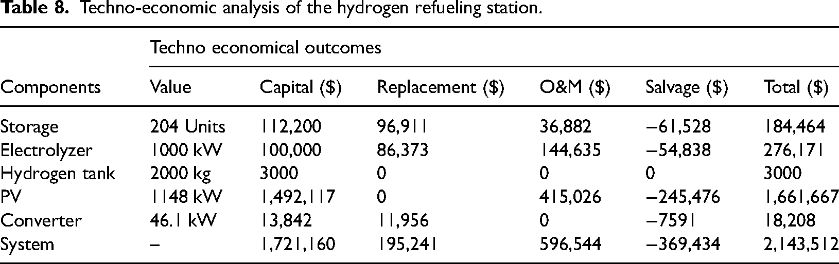
The simulation results demonstrate the basic techno-economic and operational feasibility of the suggested HRS, which is tailored for solar PV energy integration. The system's estimated total NPC over its anticipated lifecycle is 2,143,512 $, as shown in Table 8. This sum includes salvage values, operation and maintenance (O&M) expenses, capital investment, and component replacement. The PV system accounts for the largest portion of the investment among the components, at about 1,661,667 $, highlighting the importance of clean electricity in promoting the viability of renewable hydrogen. The energy storage components, which include 204 battery units and a 2000 kg hydrogen tank, add 187,464 $ to the total cost, while the 1000 kW PEM electrolyzer accounts for 276,171 $. With an LCOH of 3.20 $/kg, the system is highly economically competitive when compared to other renewable-integrated systems and traditional hydrogen pathways. Importantly, this price is consistent with long-term decarbonization plans since it represents a completely renewable architecture free from reliance on fossil fuel-based grid electricity. Economic sustainability depends on an efficient, demand-responsive design that reduces energy losses and overproduction, as evidenced by the close match between annual hydrogen production (36,998 kWh) and consumption (36,476 kWh). Comparing the suggested system's values with those published in the literature highlights its competitiveness even more. In a wind-based hydrogen production system limited by less-than-ideal wind resources, Ayodele et al.⁹⁹ reported an LCOH of 8.02 $/kg. While Rasool et al.¹⁰⁰ reported an LCOH of 9.52 $/kg for a similar PV–wind turbine (WT) system in Pakistan, Hussam et al.¹⁰¹ found an LCOH of 6.85 $/kg for a PV–WT hybrid configuration. On the other hand, the much lower LCOH of the current system demonstrates the combined benefit of Jiangsu Province's advantageous solar conditions as well as the hybrid VMD-SE-BBO-HGBR model. Through precise, real-time alignment between generation and electrolyzer operation made possible by DNI's improved forecasting accuracy, excess energy use and operational inefficiencies are decreased, enhancing system reliability and economic viability.

Table 8.

Techno-economic analysis of the hydrogen refueling station.

Components	Techno economical outcomes
Components	Value	Capital ($)	Replacement ($)	O&M ($)	Salvage ($)	Total ($)
Storage	204 Units	112,200	96,911	36,882	−61,528	184,464
Electrolyzer	1000 kW	100,000	86,373	144,635	−54,838	276,171
Hydrogen tank	2000 kg	3000	0	0	0	3000
PV	1148 kW	1,492,117	0	415,026	−245,476	1,661,667
Converter	46.1 kW	13,842	11,956	0	−7591	18,208
System	–	1,721,160	195,241	596,544	−369,434	2,143,512

To further clarify the techno-economic findings, Table 9 presents the estimated LCOH corresponding to different solar irradiance forecasting models utilized in system operation. The LCOH was estimated by scaling relative to the model performance metrics, including R², RMSE, and MAPE, with the VMD-SE-BBO-HGBR model serving as the best model at 3.20 $/kg.

Table 9.

Techno-economic analysis of the hydrogen refueling station.

Model	R ²	RMSE	MAPE	MAE	Estimated LCOH ($/kg)
SARIMAX	0.80	116.96	13.36	79.08	6.75
GRU	0.86	98.02	12.23	51.79	5.92
HGBR	0.91	75.69	10.45	51.20	4.80
BBO-HGBR	0.93	67.21	6.28	43.42	4.10
VMD-BBO-HGBR	0.95	53.95	5.19	32.87	3.60
VMD-SE-BBO-HGBR	0.98	39.69	2.65	21.21	3.20

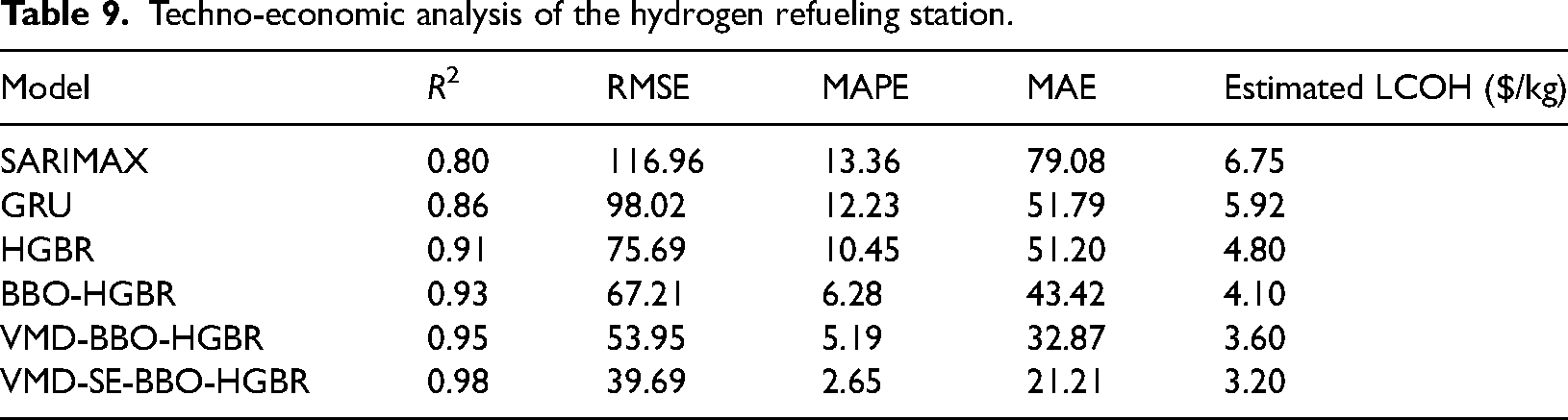
The results indicate that higher forecasting accuracy significantly improves the economic viability of the hydrogen refueling system. Accurate predictions enable better alignment between solar energy generation and electrolyzer operation, reducing excess energy storage requirements and operational inefficiencies. Consequently, improved forecasting directly translates into lower capital and operational expenditures, reflected in the reduced LCOH values. This techno-economic advantage highlights the importance of deploying advanced forecasting models such as the hybrid VMD-SE-BBO-HGBR to achieve cost-effective and sustainable renewable hydrogen production.

Table 10 indicates that the system exhibits high efficiency in hydrogen generation, with its consumption rate. The electrolyzer generates 36,998 kWh/year of hydrogen energy, which is used at full capacity. This output aligns precisely with hydrogen consumption, totaling 36,476 kWh/year. This implies that no resources are squandered, demonstrating the system's efficiency in fulfilling hydrogen demand for car refueling and energy storage without excess production.

Table 10.

Annual hydrogen and electrical energy production and consumption of the hybrid microgrid system.

Hydrogen production	kWh/yr	%	Hydrogen consumption	kWh/yr	%
Electrolyzer	36,998	100	Hydrogen load	36,476	100
Total	36,998	100	Total	36,476	100
Electrical Production	kWh/yr	%	Electrical Consumption	kWh/yr	%
PV	1,906,153	100	AC Primary Load	27,696	1.59
Total	1,906,153	100	Total	1,744,599	100

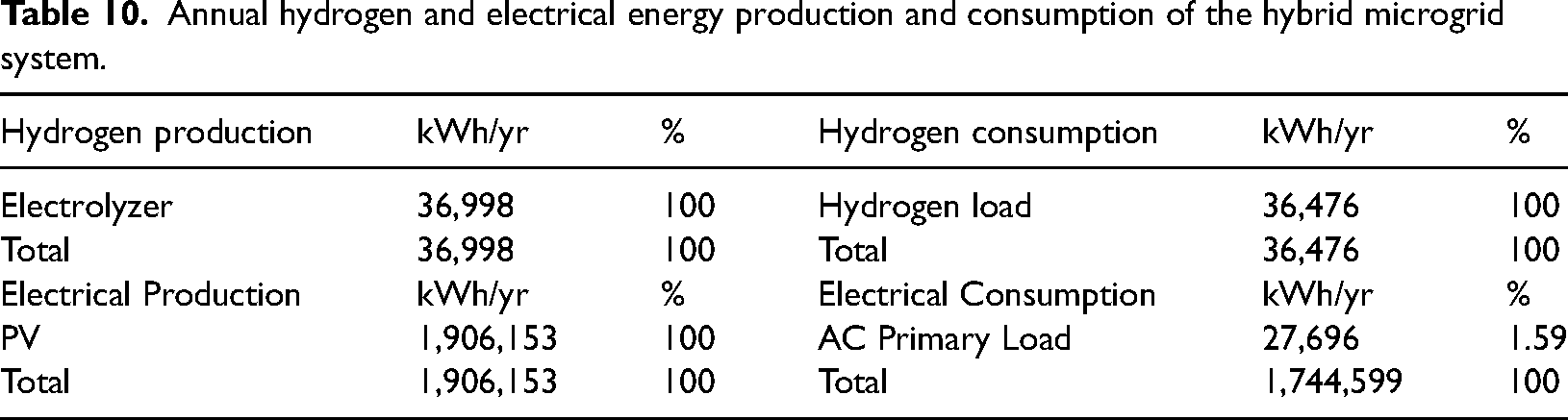
The electrical performance of the photovoltaic system is encapsulated in Table 10. A total of 1,906,153 kWh/year of power is produced, fulfilling all electrical requirements while supporting hydrogen synthesis. A mere 27,696 kWh/year (1.59%) is allocated to the main AC load, which is not intended consumption but rather for the operation of various components in the hydrogen production process. The majority of the energy is dedicated to hydrogen generation processes. The system, while very efficient, generates an excess of 159,592 kWh annually. The surplus may be further enhanced by demand-side management tactics or supplementary energy storage options integrated into the system. The system has a capacity shortfall of just 11.7 kWh/year, signifying that the design is very dependable and the level of unmet energy demand is negligible. The simulation results demonstrate the system's capacity to optimize renewable energy use while maintaining operational dependability. The model used sophisticated technology to achieve equilibrium among energy generation, storage, and utilization. The system mitigates energy fluctuations by converting surplus energy into hydrogen and using high-capacity storage to provide a reliable supply for car refueling and other energy applications. The competitive LCOH and economical NPC of the system indicate its operational viability and financial feasibility. Moreover, the system's design flexibility enables scalability to accommodate varying energy needs and potential future expansions.

The temporal dynamics and operational features of the hydrogen refueling station are visualized the system's performance across different timeframes and operational parameters. Figure 19 depicts the annual distribution of PV power production, ranging from 0 to around 1350 kW. The heat map illustrates diurnal and seasonal trends in power production, with greater intensities (shown by lighter hues) during peak sun hours and summer months. Figure 19 reflects the system's PV capacity of 1148 kW as shown in Table 10, illustrating the actual operating performance of the installed capacity. The cyclical variations in power input and storage capacities illustrate the system's capability to equilibrate output and demand, sustaining operating efficiency despite the inconsistency of renewable energy sources. The storage configurations conform to the system's design specifications, using 204 storage units with an aggregate hydrogen tank capacity of 2000 kg, therefore guaranteeing a dependable supply for vehicle refueling purposes.

Figure 19.

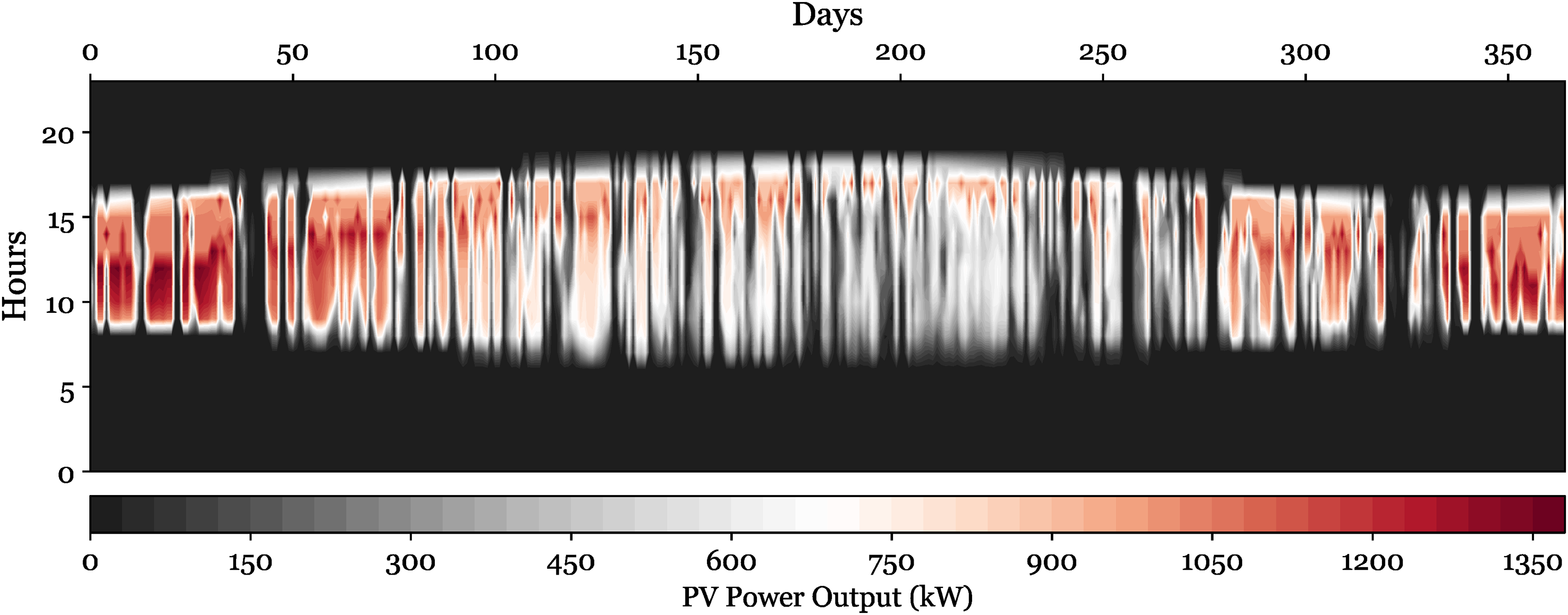
Annual photovoltaic power output distribution across hours and days.

Figure 20 illustrates the monthly variations in input power for the electrolyzer, highlighting the system's operating dynamics. The twelve-monthly subplots, each illustrating power intake patterns from 0 to 800 kW. The periodic fluctuations in power input correspond with daily solar availability patterns, while the differing amplitudes across the months indicate seasonal differences in solar resource availability. This corresponds with the total yearly electricity output of 1,906,153 kWh/year shown in Table 10, illustrating the system's ability to efficiently harness solar energy for hydrogen synthesis. Figure 21 illustrates a heat map representation of hydrogen storage levels throughout the course of the year, with values spanning from 0 to 1920 kg. The color gradient, illustrates clear seasonal variations in hydrogen storage. Significant buildup transpires throughout the summer months (May-August), as seen by the dominating yellow areas, indicating favorable circumstances for solar energy conversion. In contrast, the deeper blue areas during the winter months (November-January) indicate diminished storage levels, associated with less solar availability and perhaps increased demand. Figure 22 displays a histogram with a superimposed probability density curve illustrating the frequency distribution of stored hydrogen levels. The distribution has bimodal traits, with a modest peak at around 1000 kg and a prominent peak close to 2000 kg storage capacity. This distribution pattern indicates that the system often functions at elevated storage levels, signifying efficient hydrogen generation and storage management.

Figure 20.

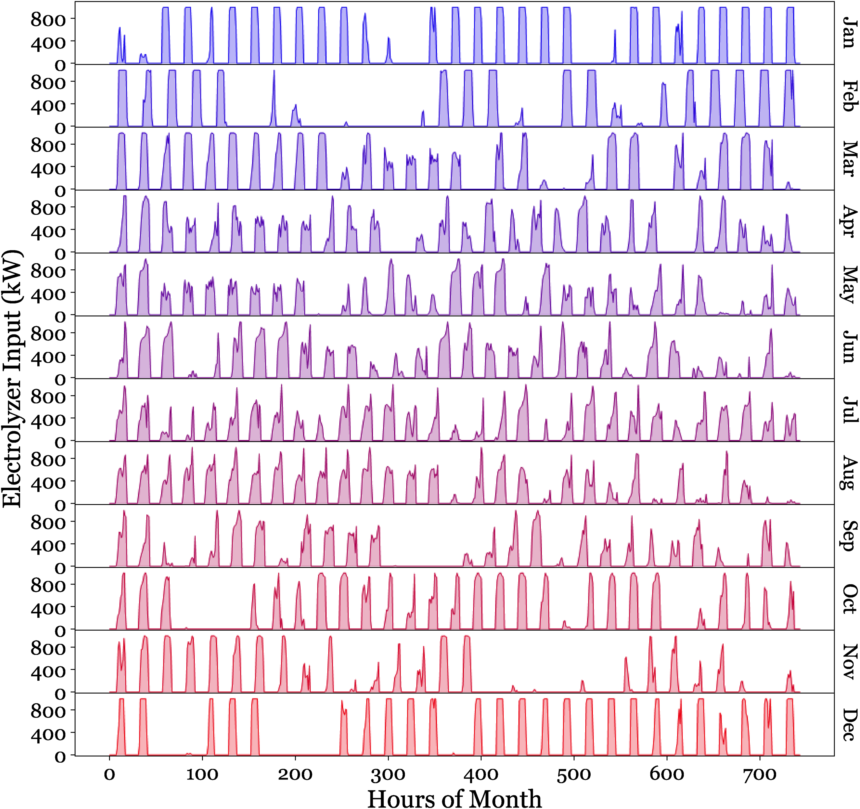
Monthly electrolyzer power input profiles throughout the year.

Figure 21.

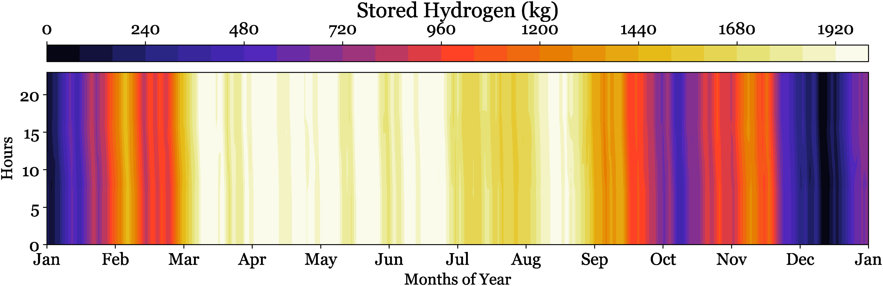
Temporal distribution of stored hydrogen levels across a year.

Figure 22.

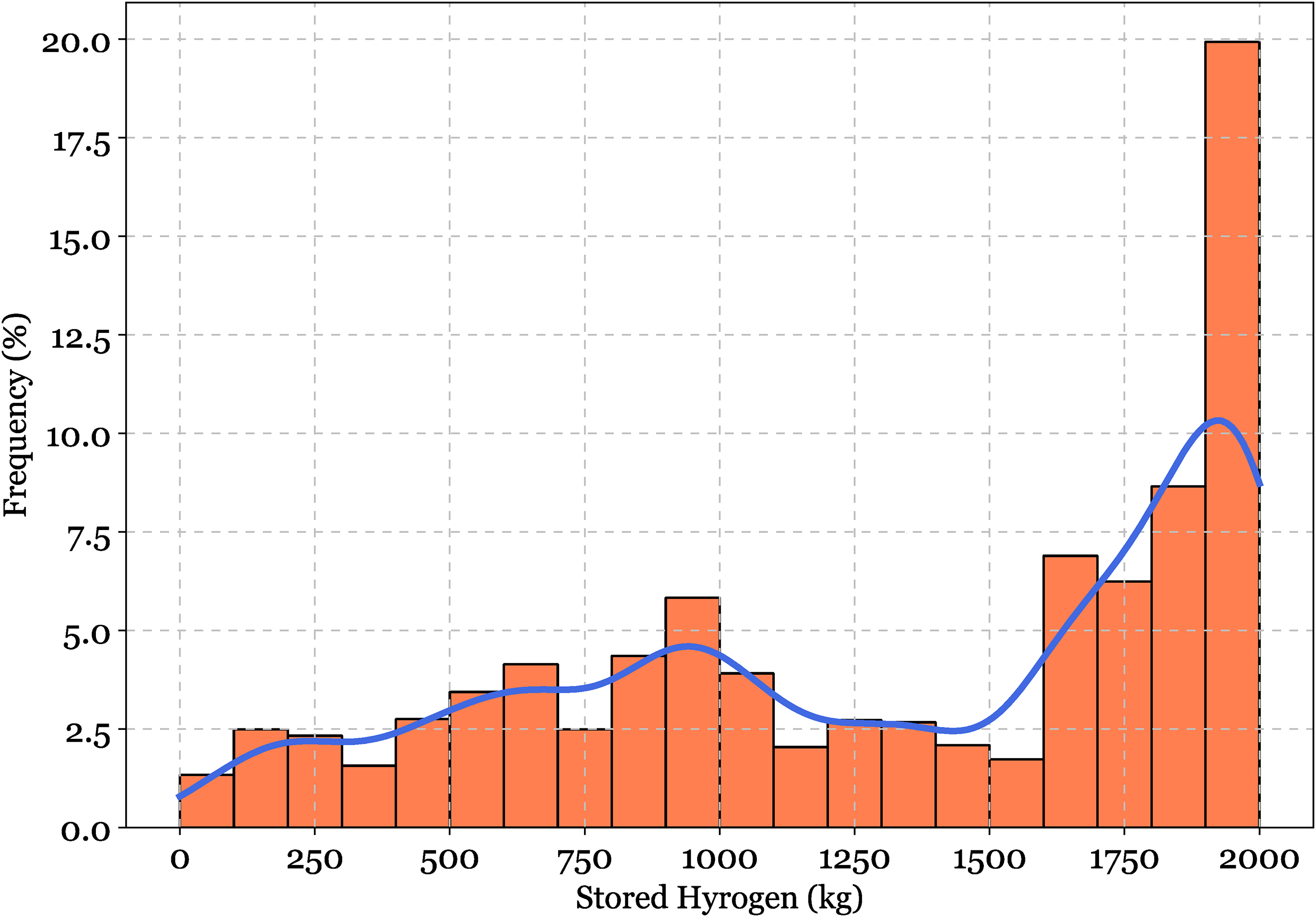
Frequency distribution of stored hydrogen levels with probability density overlay.

Figure 23 illustrates the inverter power output throughout the year, exhibiting stable functioning patterns between 2 and 12 kW. The dispersed point distribution illustrates the fluctuating nature of power conversion demands, with a concentrated cluster at 4–8 kW signifying standard functioning ranges. This pattern corresponds with the system's electrical consumption profile shown in simulation findings, whereby 27,696 kWh/year is designated for the AC main load, constituting 1.59% of overall electrical consumption. Figure 24 displays a dual-panel representation of the battery system's performance over the course of one year (8760 h). The battery state of charge (%), generally remaining elevated between 80–100%, with occasional deep discharges shown by abrupt downward spikes illustrated. The charging (green) and discharging (red) power profiles, reaching maxima of around 150 kW are depicted. This cycle pattern illustrates the battery's function in mitigating short-term variations in renewable energy production and system demand, facilitating the electrolyzer's operation during times of inconsistent solar availability.

Figure 23.

Temporal distribution of inverter power output throughout the year, illustrating the dynamic power conversion requirements for system operation.

Figure 24.

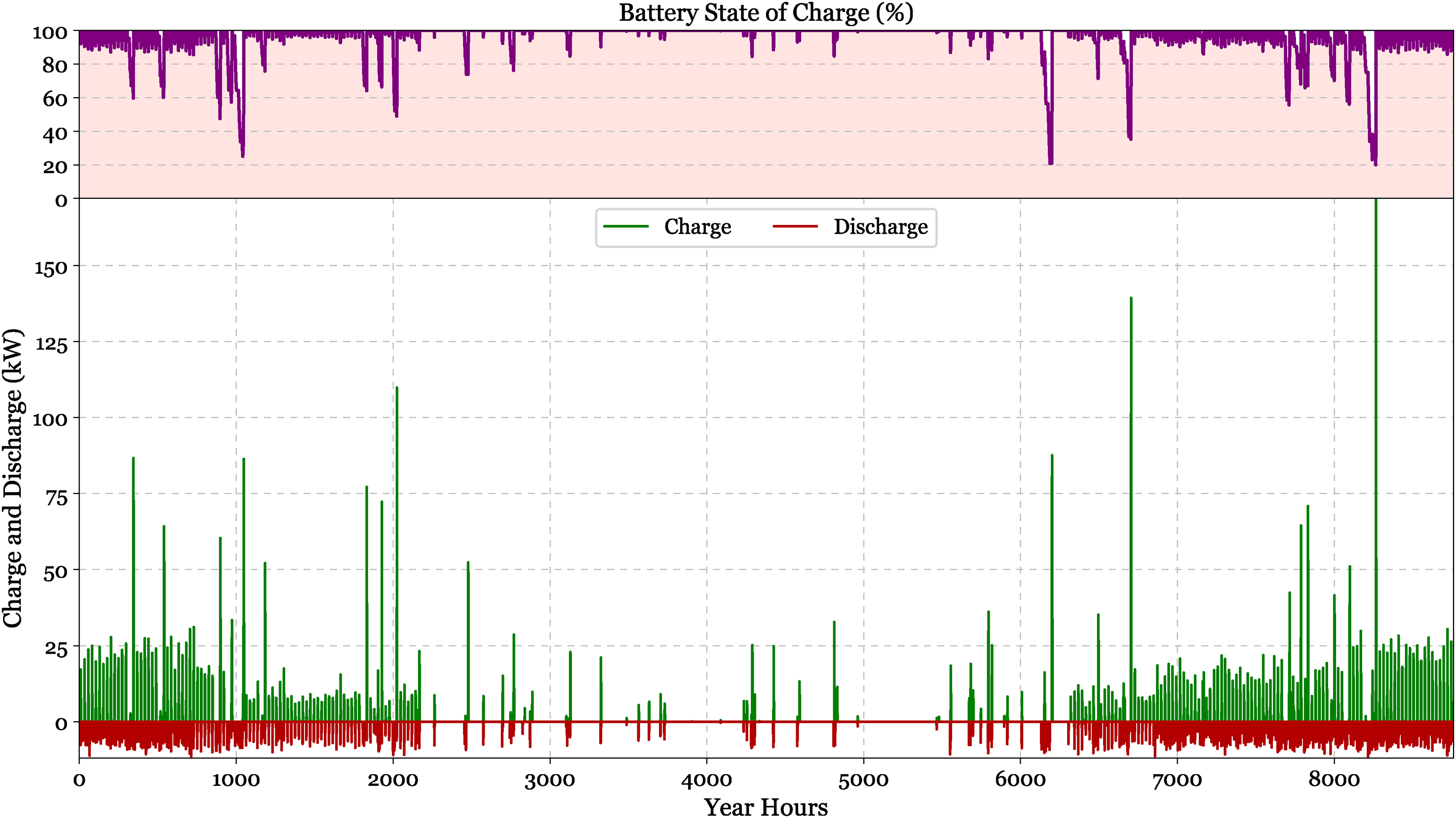
Annual battery performance profile showing state of charge variations and charging/discharging power dynamics.

The 3.20 $/kg LCOH that was attained is indicative of a promising level of economic performance for a fully renewable, solar-integrated HRS. This cost positions the system below numerous renewable hydrogen projects that have been reported in the literature and brings it closer to international cost targets. Hydrogen fuel becomes increasingly viable for medium- to large-scale applications, such as fleet-based transportation, at this level, particularly in regions with high solar resource availability, such as Jiangsu Province. A substantial but potentially manageable investment is indicated by the NPC of 2,143,512 $ when amortized over the station's operational duration and scaled across multiple deployment sites. The system's low operational costs are a result of its minimal external electricity requirements and reliance on free solar energy, which is in contrast to conventional fossil-based hydrogen production methods. These results underscore the economic viability of decentralized hydrogen infrastructure, particularly when accompanied by policies that reduce capital costs or increase the value of avoided emissions. Additionally, the system's cost-effectiveness is further reinforced by the integration of precise DNI forecasting, which leads to improved system reliability, operational efficiency, and tighter load matching.

From a systems-level and policy perspective, the results of this study add to the expanding knowledge of how integrated renewable-hydrogen systems can be both economically and technically feasible in practical operating environments. In the solar-rich environment of Jiangsu Province, the suggested HRS model, which is based on a decentralized, solar-powered architecture, shows how such systems can reach a competitive LCOH of 3.20 $/kg. The findings, though context-specific, imply that optimized renewable-hydrogen configurations might provide an economically feasible path to low-carbon and more resilient transportation infrastructure. Targeted policy interventions can be crucial to promoting wider deployment, especially in developing hydrogen economies. Improving cost structures and investment appeal would be achieved by lowering capital expenditure through subsidies for PV modules, PEM electrolyzers, and energy storage systems. Furthermore, considering their function in improving techno-economic performance, decreasing inefficiencies, and boosting system responsiveness, digital infrastructure initiatives could facilitate the integration of advanced forecasting models, like the VMD-SE-BBO-HGBR framework presented in this study. While replication feasibility will differ by region, the system architecture's scalability and modularity offer a solid basis for adaptation in various economic and geographic contexts. Planning for hydrogen supply chains, distributed energy systems, and mobility hubs could benefit from the methodology described in this study, especially as countries work to operationalize long-term decarbonization goals and national hydrogen roadmaps. In conclusion, this research highlights how crucial it is to incorporate component-level optimization, localized resource modeling, and data-driven forecasting into the design of upcoming green hydrogen systems. Realizing the full potential of hydrogen as an essential component of the global clean energy transition may require the convergence of these technical components under a logical policy and planning framework.

Conclusions

This study proposed a novel hybrid forecasting model—VMD-SE-BBO-HGBR—for accurate prediction of DNI, aimed at improving the efficiency and reliability of solar energy integration into HRSs in Jiangsu Province, China. The model combines VMD and SE for signal decomposition and feature clustering, while BBO is used to optimize HGBR parameters. This integrated structure significantly enhances the accuracy of short-term solar irradiance forecasting. The improved DNI forecasting directly supports the operational optimization of the HRS. The proposed model achieved an R² of 0.98, with RMSE and MAE of 39.69 W/m² and 21.21 W/m², respectively. This high forecasting accuracy enables more effective scheduling of energy flows and electrolyzer operation, minimizing curtailment and improving system efficiency. Informed by these forecasts, the HRS system includes a 1148 kW PV array, a 1000 kW PEM electrolyzer, a 204-kWh battery storage unit, and a 2000 kg hydrogen tank. Simulation results indicate that the system can meet a hydrogen demand of up to 100 kg/day with minimal energy shortfall. Economically, the system achieves an NPC of 2,143,512 $ and an LCOH of 3.20 $/kg, positioning it as a competitive renewable hydrogen solution when compared to similar systems reported in the literature. Beyond its numerical performance, the proposed model demonstrates adaptability across varying meteorological conditions, while the system's modular design offers flexibility for scale-up and regional replication. The integration of accurate forecasting with optimized component sizing enhances energy utilization, cost control, and operational stability. This work delivers both a high-performance solar forecasting approach and a techno-economically feasible HRS design. It offers a replicable framework for deploying solar-powered hydrogen infrastructure in favorable irradiance zones. Future research may focus on real-time implementation, cross-regional validation, and integration with demand-side and policy-driven strategies to further reduce hydrogen costs and support clean energy transitions.

Footnotes

Declaration of conflicting interests

The authors declared no potential conflicts of interest with respect to the research, authorship, and/or publication of this article.

Funding

The authors received no financial support for the research, authorship, and/or publication of this article.

ORCID iD

Xiaoshuang Hu

Wen Wu is a Lecturer in English Language and Translation. Her area of research is College English teaching, English translation, and second language acquisition.

Xiaoshuang Hu is a Lecturer in Information and Telecommunication Engineering. Her area of research includes computer graphic design, computer software development, and optimization algorithms for HEVC.

Nomenclature

References

Siyal

Mentis

Howells

. Economic analysis of standalone wind-powered hydrogen refueling stations for road transport at selected sites in Sweden. Int J Hydrogen Energy 2015; 40: 9855–9865.

Ghaithan

Kondkari

Mohammed

, et al. Optimal design of concentrated solar power-based hydrogen refueling station: mixed integer linear programming approach. Int J Hydrogen Energy 2024; 86: 703–718.

Kouchachvili

Yaïci

Entchev

. Hybrid battery/supercapacitor energy storage system for the electric vehicles. J Power Sources 2018; 374: 237–248.

Kyriakopoulos

. Energy communities overview: Managerial policies, economic aspects, technologies, and models. J Risk Financ Manag 15, Epub ahead of print 2022. DOI: https://doi.org/10.3390/jrfm15110521

Kyriakopoulos

Aravossis

. Literature Review of Hydrogen Energy Systems and Renewable Energy Sources. Energies (Basel) 16, Epub ahead of print 2023. DOI: https://doi.org/10.3390/en16227493

International Energy Agency I. Global Hydrogen Review 2021, www.iea.org/t&c/ .

Cano

Banham

, et al. Batteries and fuel cells for emerging electric vehicle markets. Nat Energy 2018; 3: 279–289.

Alazemi

Andrews

. Automotive hydrogen fuelling stations: an international review. Renewable Sustainable Energy Rev 2015; 48: 483–499.

Ruth

Jadun

Gilroy

, et al. The technical and economic potential of the H2@Scale hydrogen concept within the United States, https://www.nrel.gov/docs/fy21osti/77610.pdf (2020).

10.

Luo

, et al. Development and application of fuel cells in the automobile industry. J Energy Storage 2021; 42: 103124.

11.

Zhang

. The development trend of and suggestions for China’s hydrogen energy industry. Engineering 2021; 7: 719–721.

12.

Zhu

Feng

, et al. Economic analysis of hydrogen refueling station considering different operation modes. Int J Hydrogen Energy 2024; 52: 1577–1591.

13.

Pan

, et al. Optimal planning for electricity-hydrogen integrated energy system considering power to hydrogen and heat and seasonal storage. IEEE Trans Sustain Energy 2020; 11: 2662–2676.

14.

Liu

. Proposing an innovative model for solar irradiance and wind speed forecasting. Appl Therm Eng 2025; 262: 125224.

15.

Choi

Bhakta

. Hybrid solar photovoltaic-wind turbine system for on-site hydrogen production: a techno-economic feasibility analysis of hydrogen refueling Station in South Korea’s climatic conditions. Int J Hydrogen Energy 2024; 93: 736–752.

16.

Ghaithan

. Multi-objective model for designing hydrogen refueling station powered using on-grid photovoltaic-wind system. Energy 2024; 312: 133464.

17.

Zúñiga-Saiz

Sánchez-Díaz

. Design of a Hydrogen Refueling Station with hydrogen production by electrolysis, storage and dispensing for a bus fleet in the city of Valencia. Int J Hydrogen Energy. Epub ahead of print 2024. DOI: https://doi.org/10.1016/j.ijhydene.2024.07.387

18.

Atabay

Devrim

. Design and techno-economic analysis of solar energy based on-site hydrogen refueling station. Int J Hydrogen Energy 2024; 80: 151–160.

19.

Hajjaji

Cristofari

. Economic and technical evaluation of on-site electrolysis solar hydrogen refueling station in Corsica: a case study of Ajaccio. Renew Energy 2024; 231: 120982.

20.

Liu

Chen

, et al. Technical and economic analysis of a hybrid PV/wind energy system for hydrogen refueling stations. Energy 2024; 303: 131899.

21.

Okonkwo

Islam

Taura

, et al. A techno-economic analysis of renewable hybrid energy systems for hydrogen production at refueling stations. Int J Hydrogen Energy 2024; 78: 68–82.

22.

Xia

Rezaei

Dampage

, et al. Techno-economic assessment of a grid-independent hybrid power plant for co-supplying a remote micro-community with electricity and hydrogen. Processes 9. Epub ahead of print 2021. DOI: https://doi.org/10.3390/pr9081375

23.

Barhoumi

. Optimal design of standalone hybrid solar-wind energy systems for hydrogen-refueling station case study. J Energy Storage 2023; 74: 109546.

24.

Troncoso

Lapeña-Rey

Valero

. Solar-powered hydrogen refuelling station for unmanned aerial vehicles: design and initial AC test results. Int J Hydrogen Energy 2014; 39: 1841–1855.

25.

Yuan

Chen

Liang

. Precise solar radiation forecasting for sustainable energy integration: a hybrid CEEMD-SCM-GA-LGBM model for day-ahead power and hydrogen production. Renew Energy 2024; 237: 121732.

26.

Salehinejad

Sankar

Barfett

, et al. Recent advances in recurrent neural networks. arXiv preprint arXiv:180101078.

27.

Kumari

Toshniwal

. Deep learning models for solar irradiance forecasting: a comprehensive review. J Clean Prod 2021; 318: 128566.

28.

Mandic

Chambers

. Recurrent neural networks for prediction: learning algorithms, architectures and stability. Chichester: Wiley, 2001.

29.

Sibtain

Saleem

, et al. A multistage hybrid model ICEEMDAN-SE-VMD-RDPG for a multivariate solar irradiance forecasting. IEEE Access 2021; 9: 37334–37363.

30.

Pereira

Canhoto

Salgado

. Development and assessment of artificial neural network models for direct normal solar irradiance forecasting using operational numerical weather prediction data. Energy and AI 2024; 15: 100314.

31.

Rodríguez

Droguett

Cardemil

, et al. Enhancing the estimation of direct normal irradiance for six climate zones through machine learning models. Renew Energy 2024; 231: 120925.

32.

Jeon

B-K

Kim

E-J

. Solar irradiance prediction using reinforcement learning pre-trained with limited historical data. Energy Reports 2023; 10: 2513–2524.

33.

Jacques Molu

Tripathi

Mbasso

, et al. Advancing short-term solar irradiance forecasting accuracy through a hybrid deep learning approach with Bayesian optimization. Results in Engineering 2024; 23: 102461.

34.

Gao

Huang

Shi

, et al. Hourly forecasting of solar irradiance based on CEEMDAN and multi-strategy CNN-LSTM neural networks. Renew Energy 2020; 162: 1665–1683.

35.

Puah

Chong

Wong

, et al. A regression unsupervised incremental learning algorithm for solar irradiance prediction. Renew Energy 2021; 164: 908–925.

36.

Lee

Wang

Harrou

, et al. Reliable solar irradiance prediction using ensemble learning-based models: a comparative study. Energy Convers Manag 2020; 208: 112582.

37.

Yang

Shi

. Underwater acoustic signal denoising model based on secondary variational mode decomposition. Defence Technology 2023; 28: 87–110.

38.

Guo

Meng

Wang

, et al. Landslide displacement prediction based on variational mode decomposition and GA–Elman Model. Appl Sci (Switzerland) 13. Epub ahead of print 2023. DOI: https://doi.org/10.3390/app13010450

39.

Yang

Cheng

. A new traffic flow prediction model based on cosine similarity variational mode decomposition, extreme learning machine and iterative error compensation strategy. Eng Appl Artif Intell 2022; 115: 105234.

40.

Wang

Chen

, et al. Monthly ship price forecasting based on multivariate variational mode decomposition. Eng Appl Artif Intell 2023; 125: 106698.

41.

Liu

Huang

Tian

, et al. A stock series prediction model based on variational mode decomposition and dual-channel attention network. Expert Syst Appl 2024; 238: 121708.

42.

Shi

Sibtain

, et al. A hybrid forecasting model for short-term power load based on sample entropy, two-phase decomposition and whale algorithm optimized support vector regression. IEEE Access 2020; 8: 166907–166921.

43.

Jawed

Sajid

. Enhancing the cryptographic key using sample entropy and whale optimization algorithm. Int J Inf Technol 2024; 16: 1733–1741.

44.

Bansal

Sangtani

Dadheech

, et al. Biogeography-based optimization of artificial neural network (BBO-ANN) for solar radiation forecasting. Appl Artif Intell 2023; 37: 2166705.

45.

Zhang

Gao

Liu

, et al. A hybrid biogeography-based optimization algorithm to solve high-dimensional optimization problems and real-world engineering problems. Appl Soft Comput 2023; 144: 110514.

46.

Reihanian

Feizi-Derakhshi

Aghdasi

. An enhanced multi-objective biogeography-based optimization for overlapping community detection in social networks with node attributes. Inf Sci (N Y) 2023; 622: 903–929.

47.

Liao

Chen

, et al. Enhanced battery health monitoring in electric vehicles: a novel hybrid HBA-HGBR model. J Energy Storage 2025; 110: 115316.

48.

Zheng

Zhou

, et al. Predictive analytics for sustainable energy: an in-depth assessment of novel stacking regressor model in the off-grid hybrid renewable energy systems. Energy 2025; 324: 135916.

49.

Klaar

ACR

Stefenon

Seman

, et al. Structure optimization of ensemble learning methods and seasonal decomposition approaches to energy price forecasting in Latin America: a case study about Mexico. Energies (Basel) 2023; 16: 3184.

50.

Zippenfenig

. Open-Meteo.com Weather API. Epub ahead of print 4 July 2023. DOI: https://doi.org/10.5281/ZENODO.8112599

51.

Senthilnathan

. USEFULNESS OF CORRELATION ANALYSIS Samithambe Senthilnathan.

52.

Alsharif

Younes

Kim

. Time series ARIMA model for prediction of daily and monthly average global solar radiation: the case study of Seoul, South Korea. Symmetry (Basel) 2019; 11: 240.

53.

Alharbi

Csala

. A Seasonal autoregressive integrated moving average with exogenous factors (SARIMAX) forecasting model-based time series approach. Inventions 7. Epub ahead of print 2022. DOI: https://doi.org/10.3390/inventions7040094

54.

Sheng

Xie

Zhou

, et al. A hybrid model based on complete ensemble empirical mode decomposition with adaptive noise, GRU network and whale optimization algorithm for wind power prediction. IEEE Access 2023; 11: 62840–62854.

55.

Faisal

ANMF

Rahman

Habib

MTM

, et al. Neural networks based multivariate time series forecasting of solar radiation using meteorological data of different cities of Bangladesh. Results in Engineering 2022; 13: 100365.

56.

Cho

Van Merriënboer

Gulcehre

, et al. Learning phrase representations using RNN encoder-decoder for statistical machine translation. arXiv preprint arXiv:14061078.

57.

Bentéjac

Csörgő

Martínez-Muñoz

. A comparative analysis of gradient boosting algorithms. Artif Intell Rev 2021; 54: 1937–1967.

58.

Liang

Luo

Zhao

, et al. Predicting Hard Rock Pillar Stability Using GBDT, XGBoost, and LightGBM Algorithms. Mathematics 8. Epub ahead of print 2020. DOI: https://doi.org/10.3390/math8050765

59.

Rao

Shi

Rodrigue

, et al. Feature selection based on artificial bee colony and gradient boosting decision tree. Appl Soft Comput 2019; 74: 634–642.

60.

Nhat-Duc

Van-Duc

. Comparison of histogram-based gradient boosting classification machine, random forest, and deep convolutional neural network for pavement raveling severity classification. Autom Constr 2023; 148: 104767.

61.

Guryanov

. Histogram-based algorithm for building gradient boosting ensembles of piecewise linear decision trees. In: Analysis of Images, Social Networks and Texts: 8th International Conference, AIST 2019, Kazan, Russia, July 17–19, 2019, Revised Selected Papers 8, Springer, 2019, pp.39–50.

62.

Liu

Huang

, et al. Hourly stepwise forecasting for solar irradiance using integrated hybrid models CNN-LSTM-MLP combined with error correction and VMD. Energy Convers Manag 2023; 280: 116804.

63.

Sun

Liu

. Multivariate short-term wind speed prediction based on PSO-VMD-SE-ICEEMDAN two-stage decomposition and Att-S2S. Energy 2024; 305: 132228.

64.

Dragomiretskiy

Zosso

. Variational mode decomposition. IEEE Trans Signal Process 2014; 62: 531–544.

65.

Cui

Jia

Pang

, et al. A data-driven method with sample entropy and CEEMDAN for short-term performance degradation prediction of dynamic hydrogen fuel cells. Int J Hydrogen Energy 2024; 83: 916–932.

66.

Liu

. A novel hybrid model based on GA-VMD, sample entropy reconstruction and BiLSTM for wind speed prediction. Measurement ( Mahwah N J) 2023; 222: 113643.

67.

Garg

Deep

Alnowibet

, et al. Biogeography based optimization with Salp Swarm optimizer inspired operator for solving non-linear continuous optimization problems. Alexandria Eng J 2023; 73: 321–341.

68.

Simon

. Biogeography-based optimization. IEEE Trans Evol Comput 2008; 12: 702–713.

69.

Wang

Zhang

, et al. Hybrid solar radiation forecasting model with temporal convolutional network using data decomposition and improved artificial ecosystem-based optimization algorithm. Energy 2023; 280: 128171.

70.

Yan

Shen

Wang

, et al. Short-term solar irradiance forecasting based on a hybrid deep learning methodology. Information (Switzerland) 2020; 11: 1–13.

71.

Zhou

Zhang

Yang

, et al. Short-Term photovoltaic power forecasting based on long short term memory neural network and attention mechanism. IEEE Access 2019; 7: 78063–78074.

72.

Khosravani

Safaei

Reynolds

, et al. Challenges of reaching high renewable fractions in hybrid renewable energy systems. Energy Reports 2023; 9: 1000–1017.

73.

Islam

Akhter

Rahman

. A thorough investigation on hybrid application of biomass gasifier and PV resources to meet energy needs for a northern rural off-grid region of Bangladesh: a potential solution to replicate in rural off-grid areas or not? Energy 2018; 145: 338–355.

74.

Vergara-Zambrano

Kracht

Díaz-Alvarado

. Integration of renewable energy into the copper mining industry: a multi-objective approach. J Clean Prod 2022; 372: 133419.

75.

Kasaeian

Rahdan

Rad

MAV

, et al. Optimal design and technical analysis of a grid-connected hybrid photovoltaic/diesel/biogas under different economic conditions: a case study. Energy Convers Manag 2019; 198: 111810.

76.

Khadem

Billah

SMB

Barua

, et al. HOMER Based hydrogen fuel cell system design for irrigation in Bangladesh. In: 2017 4th International Conference on Advances in Electrical Engineering (ICAEE), 2017, pp.445–449.

77.

De León

Ríos

Brey

. Cost of green hydrogen: limitations of production from a stand-alone photovoltaic system. Int J Hydrogen Energy 2023; 48: 11885–11898.

78.

Chaudhary

Bhardvaj

Chaudhary

. A qualitative assessment of hydrogen generation techniques for fuel cell applications. Fuel 2024; 358: 130090.

79.

Tariq

Kazmi

SAA

Hassan

, et al. Analysis of fuel cell integration with hybrid microgrid systems for clean energy: a comparative review. Int J Hydrogen Energy 2024; 52: 1005–1034.

80.

Sadeghian

Shotorbani

Ghassemzadeh

, et al. Energy management of hybrid fuel cell and renewable energy based systems - A review. Int J Hydrogen Energy 2025; 107: 135–163.

81.

Ioroi

Yasuda

Siroma

, et al. Thin film electrocatalyst layer for unitized regenerative polymer electrolyte fuel cells. J Power Sources 2002; 112: 583–587.

82.

Babaei

Ting

DS-K

Carriveau

. Optimization of hydrogen-producing sustainable island microgrids. Int J Hydrogen Energy 2022; 47: 14375–14392.

83.

Babaei

Ting

DSK

Carriveau

. Feasibility and optimal sizing analysis of stand-alone hybrid energy systems coupled with various battery technologies: a case study of Pelee Island. Energy Reports 2022; 8: 4747–4762.

84.

Köprü

Öztürk

Yildirim

. Techno-economic analysis of a hybrid system for rural areas: Electricity and heat generation with hydrogen and battery storage. Int J Hydrogen Energy. Epub ahead of print 2024. DOI: https://doi.org/10.1016/j.ijhydene.2024.11.394

85.

Toghyani

Saadat

. From challenge to opportunity: Enhancing oil refinery plants with sustainable hybrid renewable energy integration. Energy Convers Manag 305. Epub ahead of print 1 April 2024. DOI: https://doi.org/10.1016/j.enconman.2024.118254

86.

Moghaddam

MJH

Kalam

Nowdeh

, et al. Optimal sizing and energy management of stand-alone hybrid photovoltaic/wind system based on hydrogen storage considering LOEE and LOLE reliability indices using flower pollination algorithm. Renew Energy 2019; 135: 1412–1434.

87.

Framework

. UNCTAD framework for sustainable freight transport (unctad sft framework).

88.

Zheng

, et al. Techno-economic feasibility study of autonomous hybrid wind/PV/battery power system for a household in Urumqi, China. Energy 2013; 55: 263–272.

89.

Hydrogen Cars - H2.LIVE, https://h2.live/en/fahren/ (accessed 4 January 2025).

90.

Dulău

L-I

. CO2 Emissions of battery electric vehicles and hydrogen fuel cell vehicles. Clean Technologies 2023; 5: 696–712.

91.

Rezk

Alghassab

Ziedan

. An optimal sizing of stand-alone hybrid PV-fuel cell-battery to desalinate seawater at Saudi NEOM City. Processes 8. Epub ahead of print 2020. DOI: https://doi.org/10.3390/pr8040382

92.

Kapen

Nouadje

BAM

Chegnimonhan

, et al. Techno-economic feasibility of a PV/battery/fuel cell/electrolyzer/biogas hybrid system for energy and hydrogen production in the far north region of Cameroon by using HOMER pro. Energy Strategy Rev 2022; 44: 100988.

93.

Chen

Tang

, et al. Optimal design and techno-economic assessment of low-carbon hydrogen supply pathways for a refueling station located in Shanghai. Energy 2021; 237: 121584.

94.

Zhang

Niu

Zhou

, et al. Prediction method of direct normal irradiance for solar thermal power plants based on VMD-WOA-DELM. IEEE Trans Appl Supercond 2024; 34: 9002904.

95.

Zhang

Zhou

Chen

, et al. A direct normal irradiance prediction model based on VMD-WOA-ELM for concentrating solar power station. In: 2023 IEEE International Conference on Applied Superconductivity and Electromagnetic Devices (ASEMD), 2023, pp.1–3: IEEE.

96.

Zhu

Wang

Guo

, et al. Hybrid machine learning and optimization method for solar irradiance forecasting. Eng Optim 2024; 56: 1–36.

97.

Tahir

Yousaf

Tzes

, et al. Enhanced solar photovoltaic power prediction using diverse machine learning algorithms with hyperparameter optimization. Renewable Sustainable Energy Rev 2024; 200: 114581.

98.

Namrata

Kumar

. Data-Driven hyperparameter optimized extreme gradient boosting machine learning model for solar radiation forecasting. Advances in Electrical and Electronic Engineering 2023; 20: 549–559.

99.

Ayodele

Mosetlhe

Yusuff

, et al. Optimal design of wind-powered hydrogen refuelling station for some selected cities of South Africa. Int J Hydrogen Energy 2021; 46: 24919–24930.

100.

Rasool

Khan

Aurangzeb

, et al. Comprehensive techno-economic analysis of a standalone renewable energy system for simultaneous electrical load management and hydrogen generation for fuel cell electric vehicles. Energy Reports 2024; 11: 6255–6274.

101.

Hussam

Barhoumi

Abdul-Niby

, et al. Techno-economic analysis and optimization of hydrogen production from renewable hybrid energy systems: Shagaya Renewable Power Plant-Kuwait. Int J Hydrogen Energy 2024; 58: 56–68.