Yardsticks of inequality: Preferences for redistribution in advanced democracies

Abstract

This article explores how preferences for redistribution among voters are affected by the structure of inequality. There are strong theoretical reasons to believe that some voter segments matter more than others, not least the so-called median-income voter, but surprisingly little attention has been paid to directly analysing distinct income groups’ redistributive preferences. In addition, while much of the previous literature has focused on broad levels of inequality, as measured by the Gini coefficient, it is likely that individuals respond to different types of inequality in different ways. To rectify this gap, we use data from the European Social Survey and Eurostat to examine the interactive effect of income deciles and various measures of inequality. Results suggest that inequality especially affects the middle-income groups – that is, the assumed median-income voters. Moreover, not all inequality matters equally: it is inequality vis-à-vis those around the 80th percentile that shapes redistributive preferences.

Keywords

European Social Survey income ratios inequality public opinion redistributive preferences

Are voters’ preferences for redistribution shaped by inequality? The interplay between national inequality levels and voter preferences is a major theme in comparative political economy beginning with the famed Meltzer–Richard (1981) model. In recent years, a number of studies have explored whether the national level of inequality, as measured by the Gini coefficient, affects voter preferences for redistribution (e.g. Dallinger, 2010; Kenworthy and McCall, 2008; Lübker, 2007; Schmidt-Catran, 2016). Results are mixed, though the newest research generally finds that a high Gini coefficient is associated with relatively high support for redistribution.

There are two reasons to be dissatisfied with the current state of the literature. First, scholars have rarely examined the redistributive preferences of specific income groups. On the one hand, much of the work centred around the redistributive preferences of specific groups only indirectly analyses them, focusing on redistributive outcomes rather than attitudes themselves (e.g. Dallinger, 2015; Kenworthy and Pontusson, 2005; Milanovic, 2000). Assuming non-trivial slippage between redistributive outcomes and preferences, which research suggests is almost certainly the case (e.g. Bonica et al., 2013; Hacker and Pierson, 2011; Matthijs, 2016), there are clear limitations to this approach. On the other, virtually all of the extant studies that directly analyse redistributive attitudes either look at aggregate preferences of the entire population (pooling the poor, the middle class, and the rich) or examine population subgroups (e.g. Alt and Iversen, 2017; Kelly and Enns, 2010; Lupu and Pontusson, 2011; Luttig, 2013; Page et al., 2013). This general failure to study the impact of redistributive preferences across the whole of the income spectrum means that we lack a systematic understanding of who is being affected by the structure of inequality: is it the (presumed powerful) median-income voters, the poor, or maybe even the well-off?

Second and related to this, existing research typically uses the Gini coefficient as the measure of inequality (e.g. Jæger, 2013; Rueda and Stegmueller, 2016; Steele, 2015). This is a good measure to capture the overall level of national inequality, since the Gini coefficient indicates how much of society’s total earnings have to be redistributed to obtain perfect equality. It is not, however, suitable to ascertain whether and how the structure of inequality shapes popular preferences. Is it, for example, the distance to the bottom or the top of the income distribution that drives preferences, and do these effects vary across the income spectrum? Other measures exist that are much better at capturing the relative position of citizens vis-à-vis other income segments, yet they have rarely been employed.

In the next section, we outline different theoretical perspectives on how different income groups might be influenced by the structure of inequality, which we then test empirically in the remainder of the article. We do so using inequality data from Eurostat combined with survey data from the last four rounds of the European Social Survey (ESS; 2008–2014), focusing specifically on redistributive preferences. These surveys have carefully parsed data on respondents’ income that allow us to compare income deciles reliably across countries. Our key findings are twofold. First, it is the fifth and sixth income decile – what we label the median-voter segment – that appears to be affected by changes in inequality; neither the poor nor the rich are much affected by changing inequality in society, perhaps reflecting more stable baseline preferences at the bottom and top of the income distribution. Second, not all types of inequality matter equally for the median-voter segment: it is inequality vis-à-vis those around the 80th percentile that shapes redistributive preferences. By contrast, we find that the distance to the poor does not affect median-voter segment preferences, and tentatively draw similar conclusions regarding the distance to the very rich. Our results, in sum, lend additional support to recent work corroborating the Meltzer–Richard model, but also hint at why the recent explosion of the incomes of the ultra-rich has not led to a greater electoral reaction.

How inequality may affect voter preferences for redistribution

There are strong a priori reasons to suspect that the structure of inequality may matter for redistributive preferences. Assuming that voters do not simply respond to the existence of inequality as such, however, the key question is, ‘What are the significant groups with which a voter compares herself?’ In other words, what is the yardstick of inequality that voters use to form opinions about the appropriate level of redistribution?

There are a number of ways one might approach answering this question, but a natural entry point is provided by the literature focused on analysing median voter preferences (see, for example, Iversen and Soskice, 2006; Lupu and Pontusson, 2011). Within this tradition, the two most basic yardsticks are the poor and the rich, which may be defined as those below and above the median income segment respectively. Taking this research field as our starting point, it is possible to deduce several expectations as to which income distances should matter and in what direction they should move the redistributive preferences of voters at the bottom, middle and top of the income distribution. To that end, we now turn to laying out the various theories designed to explain median-voter preferences, given both their prominence in the literature and their potential broader applicability across the income spectrum, before briefly highlighting their application to other decile groups.

First, one might consider the distance to the poor, which may influence the median-income voter in two very different ways. According to the social rivalry theory proposed by Corneo and Grüner (2000), the median-income voter derives utility from living a life that she perceives as better than those at the bottom. This in turn implies that if the distance between the median-income voter and the poor decreases, the median-income voter’s utility drops because her lifestyle is now imitated by up-starts. The result is that a declining distance to the poor will lead to lower support for redistribution, since this becomes a means to keep the poor less well-off than the median-income voter. Conversely, if the distance to the poor increases, the median-income voter has less to fear from the poor in this specific sense, and can therefore let other concerns influence her redistributive preferences.

A similar set of expectations follows from work focusing on economic insecurity and support for welfare programmes (e.g. Alt and Iversen, 2017; Cusack et al., 2006). Here, the central concept is insurance: individuals are expected to become more supportive of insurance against future income loss (i.e. via welfare programmes) as their income increases, since unemployment becomes increasingly costly (see Moene and Wallerstein, 2001). This effect of course depends on the distribution of labour market risk, but in instances where risk is not entirely limited to low-income individuals, the result will be a broader base of pro-redistribution support (Rehm et al., 2012). For our purposes, this suggests – just as under Corneo and Grüner’s (2000) social rivalry theory – that as the distance between the median voter and the bottom increases (decreases), the median voter will feel that she has more to gain (lose) from redistribution. Regardless of the underlying mechanism, empirical results from Tóth and Keller (2014), who carry out the closest study to our own (albeit with only a subset of the inequality measures we examine), provide support for this interpretation.

The social affinity perspective, by contrast, predicts that the distance between the median-income voter and the poor will have exactly the opposite effect (Lupu and Pontusson, 2011). From this perspective, a key component of support for redistribution is a shared sense of fate between middle- and low-income groups. Numerous factors of course shape the likelihood of social affinity – not least ethnic and racial heterogeneity (e.g. Soroka et al., 2016). Crucially, however, inequality plays a central role, driven by two potential mechanisms (Lupu and Pontusson, 2011: 318): first, high inequality is associated with lower levels of social mobility (e.g. Andrews and Leigh, 2009), making it less likely that middle-income individuals will fear dropping into the lower classes, and second, higher inequality decreases the likelihood of having interactions with the poor, since it increases social and geographic segregation (e.g. Fischer et al., 2004). As a consequence, increases in the distance between middle- and low-income groups should result in lower levels of support for redistribution.

At the same time, the distance to the top may also affect median-income voter preferences. The most well-known argument in this line of research is proposed by Meltzer and Richard (1981), who were themselves building on earlier work by Romer (1975). Meltzer and Richard theorise that the greater the distance between median and mean income, the more supportive of redistribution the median-income voter (and, indeed, all voters with a below-the-mean income) will become. The motive here is pure self-interest. When the distance between the median and mean income is large, there is a lot of money to be gained from redistribution. In contrast, when the distance between the median and mean is low, there is comparably less to be won, and redistributive preferences should accordingly be weaker. The Meltzer–Richard model assumes that as long as there is anything to be gained, the median-income voter will support redistribution – an assumption that may help to explain why many researchers have found limited support for the model (e.g. Barth et al., 2015; Bradley et al., 2003; Kenworthy and McCall, 2008; Moene and Wallerstein, 2001).

Part of the issue here may be that the Meltzer–Richard model cannot tell us if it is the distance to certain segments that matters. This is relevant because the distance to the top may mean at least two different things. The relevant distance could, for one thing, be that to the very affluent – for example, to the top 5 percent in society. This could be called the ‘soak the rich’ thesis. Yet, most people know very little about the lifestyles enjoyed by many CEOs, as evidenced by their striking underestimation of CEO remuneration levels (McCall and Chin, 2013). In the formulation of Shapiro (2002), ‘[w]orkers do not compare themselves to their bosses in assessing their circumstances. They do not compare themselves to the rich, but rather to workers like themselves’ (p. 121). This alternative view could be called the ‘envy your brother’ thesis and implies that it is the distance to income groups much closer to the median-income voter that matters.

No matter the exact yardstick used by the median-income voter to assess the distance to the top, so far, the expectation has been that a greater distance should lead to more support for redistribution. Yet, given that many of the more unequal democracies, such as the United States, redistribute relatively little, some scholars have argued in favour of the opposite relationship (Benabou, 2000; Rodríguez, 2004; Trump, 2017). Contra the Meltzer–Richard model, Benabou (2000) and Rodríguez (2004) suggest that as inequality rises, people in fact become less pro-redistribution, since their potential gain from redistribution decreases rather than increases. Key here is the focus on de facto gains: for Benabou (2000), whenever redistribution generates real or perceived improvements of overall welfare in society, increases in inequality will lead fewer individuals to find that the welfare-enhancing effects of redistribution outweigh their income losses via taxation; while for Rodríguez (2004), voters perceive that greater inequality increases the political influence of the rich, and thus assume that redistributive expenditure will disproportionately benefit the well-off, at least vis-à-vis middle-income groups. Trump (2017), in turn, finds evidence to suggest that growing inequality might lead citizens to be increasingly accepting of large income differences, thanks to a psychological tendency towards legitimising the social system in which one lives. Regardless of the mechanism, this perspective suggests that inequality will tend to reinforce itself over time, as inequality breeds anti-redistributive attitudes – a proposition that has found empirical support in several studies of overall public preferences in the United States (Kelly and Enns, 2010; Luttig, 2013). We combine these explanations into the ‘conservative acceptance’ thesis, since they all lead to the expectation that voters will accept more fiscally conservative policies as the distance to the top grows.

Although many of the above theories were devised with reference to the median-income voter, these mechanisms should work for other income segments as well – all that is required is a relevant group with which an individual can compare herself. For instance, the social rivalry theory is likely less relevant for those at the very bottom of the income distribution, but it could be central to explaining preferences of the well-off. In contrast, the poor could be motivated by both ‘soak the rich’ and ‘envy your brother’ thinking, whereas the relevance of these theories is less obvious for the well-off (though all groups are of course quite heterogeneous, a fact we explicitly deal with below). The remainder of the paper is meant to explore these ideas.

Data

To carry out our analysis, we use data from four waves of the ESS, with 22 countries included in the overall sample. In particular, we focus on the 2008–2014 rounds, since these surveys contain a standardised question asking respondents to place themselves within their corresponding income decile.¹ The number of survey respondents ultimately included in the analysis totals 106,003, with the number of observations in a given country-wave ranging from 509 (Italy in 2010) to 2609 (Germany in 2014). The vast majority of countries in the sample (15 out of 22) are included in all four rounds, while only two (Israel and Italy) have data for but a single round. Table 2 lays out further details on the distribution of respondents across the countries and waves.

Given that our focus is on attitudes towards redistribution, we use a belief that the government should reduce inequality as our dependent variable. To that end, we look at responses to the statement ‘The government should take measures to reduce differences in income levels’ with responses on a five-point scale (recoded from zero to one) ranging from ‘strongly disagree’ to ‘strongly agree’. The distribution of responses leans considerably towards agreement: about 70 percent of respondents either agree or strongly agree (with a mean of 0.70 and a standard deviation of 0.26 in the sample).

The key explanatory variable in the analysis is the interaction between inequality and income quintile, specifically at the middle-income group. As discussed above, we incorporate a variety of inequality measures in order to explore the importance of the structure of inequality. By way of a first glance at the broad relationship here, Figure 1 compares mean levels of preferences for redistribution against Gini coefficients.² Each observation on the graph represents a country-year, and we include an ordinary least squares regression line as a preliminary indicator. The plot reveals considerable variation not only in levels of inequality, but also in mean attitudes towards redistribution – ranging from 0.49 (in Denmark, 2014) to 0.85 (in Hungary, 2010). Overall, the simple bivariate relationship suggests that higher levels of inequality are correlated with a modest increase in preferences for redistribution. At this basic level, then, the data point towards a positive impact of inequality writ large on aggregate preferences for redistribution (though see our discussion of endogeneity below).

Figure 1.

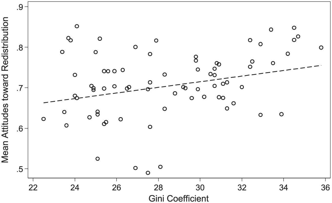
Mean attitudes towards redistribution and the Gini coefficient.

Our key goal here, however, is to disaggregate both income groups and the effects of different types of inequality, thereby permitting us to examine how the structure of inequality affects different income groups. We examine five inequality ratios that reflect our hypotheses: 50:5, 50:20, 80:50, 95:50, and 90:10.³ These measures indicate the distance between two percentile points, where lower percentiles are associated with lower income levels. The 50:20 ratio, for instance, tells us how many times higher the net income of the 50th percentile (i.e. the percentile that exactly cuts the income distribution in two) is compared to the 20th percentile. A 50:20 ratio of two indicates that those at the 50th percentile make twice as much income after taxes and transfers than those at the 20th percentile. Similarly, the 95:50 ratio tells us how many times more income the 95th percentile takes home compared to the 50th.

All of our inequality measures use post-tax and transfer household income as their base, since high-quality data of this sort are much more readily available than those on market income. Most potential measures of market inequality either lack enough respondents to provide a reliable measure of inequality (e.g. ESS data) or would force us to exclude various countries and survey waves from the analysis (e.g. LIS data). Eurostat, by contrast, has comparable alternative data to those we are using – but that measure of income distribution is only pre-social transfer (save for pensions), not pre-taxes.

These gains in data quality are, however, accompanied by two principal drawbacks. First, the use of post-tax and transfer inequality data prevent us from performing a strict test of Meltzer and Richard (1981), which places market inequality at its core. Yet, while it is certainly true that the Meltzer–Richard model assumes that people care about market inequality, the intuition behind this assumption is questionable. There are strong a priori reasons to believe that disposable income – not market income – is what drives preference for more or less redistribution: post-tax and transfer inequality is the inequality that individuals actually experience in society, and insofar as people care about the ability to maintain a specific lifestyle (compared to relevant other groups) disposable income should matter much more than market income.

Second and more fundamentally, the use of post-tax and transfer data also introduces issues of endogeneity to the model. When asked about their desire for government action to reduce income differences, at least some survey respondents are liable to take into account the current level of actually existing inequality. Although there is considerable debate as to the scope of public responsiveness (see Druckman, 2014) and even the direction such an effect might take (compare Soroka and Wlezien, 2010; Trump, 2017), it seems almost certain that some effect would be present. Cross-sectional survey analysis is ill-suited to settle these kinds of causality issues, but several considerations help to mitigate these concerns. On the one hand, as Schmidt-Catran (2016: 127–128) argues, previous research suggests that the supposed impact of using post- versus pre-tax and transfer inequality data is perhaps overstated: studies suggest that that pre- and post-tax and transfer inequality ratios are in fact quite highly correlated (e.g. Milanovic, 2000: 390; Finseraas, 2009: 101), and the empirical consequences should thus be rather limited. On the other, it is unclear why this sort of endogeneity would differentially affect the various income groups and inequality ratios under investigation here. As a consequence, we can be reasonably certain that our findings are not simply the result of our using post-tax and transfer data.

With that in mind, we calculate our inequality measures using data from the European Union Statistics on Income and Living Standards, which is collected by Eurostat via surveys and made comparable using purchasing power standard. The data provide percentile values for each of the countries. While this survey approach to formulating inequality ratios may in some cases be prone to errors on the part of respondents, the dataset has the virtue of allowing us to specify the structure of inequality in detail. Nevertheless, we attempt to circumscribe potential problems by remaining cautious about data related to the poles of the income distribution, since the quality and comparability of the data across countries becomes more suspect. This leads us to avoid anchoring inequality ratios on extreme values, such as the first and 99th percentile – partly due to difficulties including such individuals in a survey sample, but also because of measurement issues related to capital investments.⁴

The measure of respondent income decile, in turn, comes from a question in the ESS asking respondents to indicate their net household income (from all sources) within a range of values. Decile brackets were pre-calculated for each specific country-wave on the basis of the actual distribution of income preceding the survey. The distribution of decile brackets broadly reflects this construction, even after the loss of observations with missing data, with a mean decile value of 5.4 and a standard deviation of 2.8. In the final sample, most of the brackets roughly correspond to 10 percent of the observations, as we would expect, with the fifth decile the largest group (at 11.1%). And while there is some variation across countries, only in Israel does any group surpass 20 percent (with 22% of respondents in the first income decile). To address any potential issues on this front, we therefore confirm below that our results are unaffected by the inclusion of Israeli respondents.

Controls are chosen based on the standard approaches in existing research (see, for example, Cusack et al., 2006; Finseraas, 2009), so we only delineate them here briefly. At the individual level, we include standard control variables for good/very good self-assessed health status (measured as a dummy), since poor health has been found to have a positive effect on welfare state support (e.g. Jæger, 2006); self-placement on the left–right scale (on an 11-point scale, coded from 0 to 1); gender (males coded as 1), since previous research suggests females are generally more supportive of redistribution; age, with older individuals typically more supportive of redistribution; education level (using the five-category harmonised ISCED-97 scheme), since those with more education may be less precariously positioned in the labour market; dummy variables for employment and unemployment; and a dummy variable for survey wave. Finally, at the national-level, we include an economic control for (centred) gross domestic product (GDP) per capita, calculated with purchasing power parity. In line with recent work (Schmidt-Catran, 2016), we explicitly limit the number of country-level controls given limitations related both to degrees of freedom and high collinearity, instead building to a random-slopes model that allows us to control for unobserved variance that might impact the effect of our key variables.

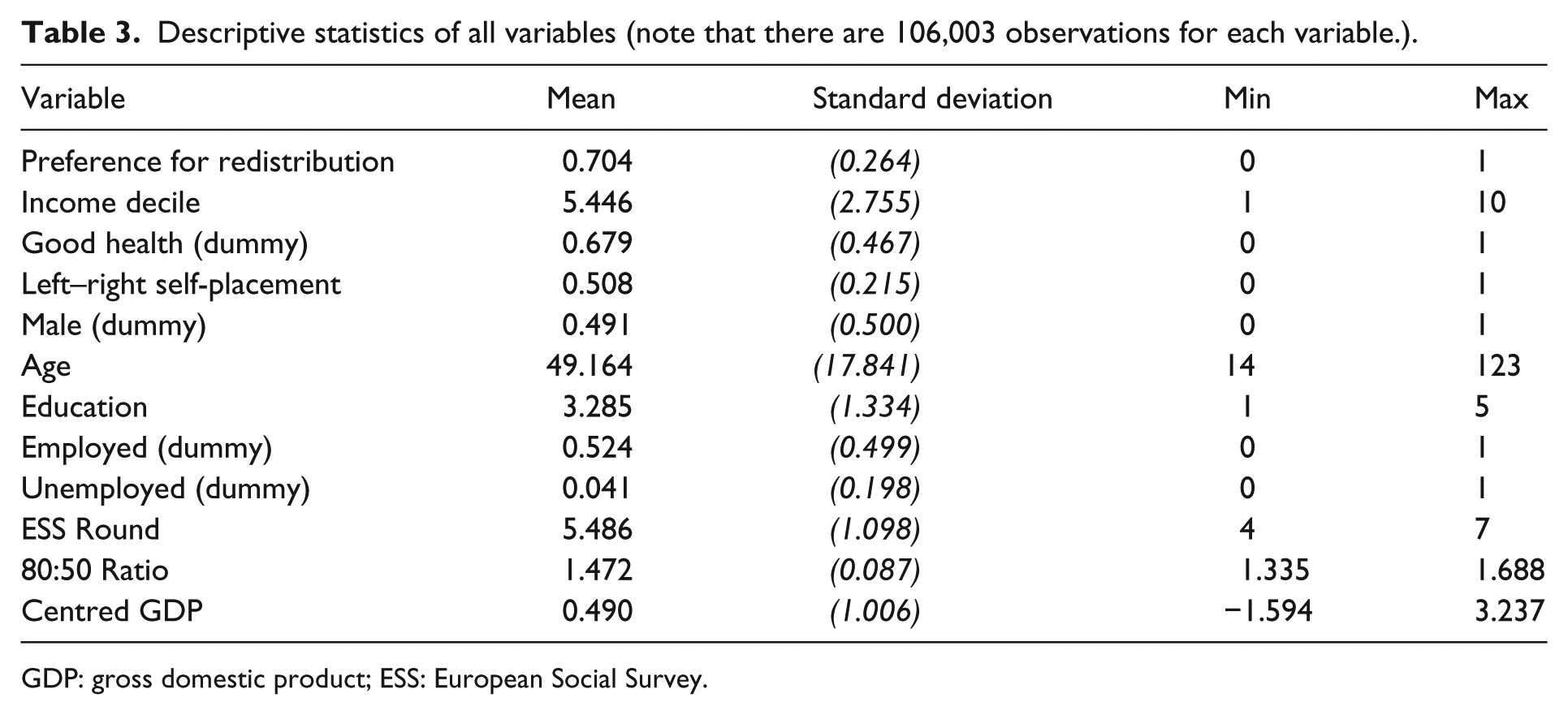
While the individual-level data of course comes directly from the ESS, the national-level data is taken from the Organisation for Economic Co-operation and Development (OECD).⁵ Note that variance inflation factor scores confirm that multicollinearity is quite low, both at the individual- and national-level, with all values below four (see O’Brien, 2007). Table 3 provides descriptive statistics for all variables incorporated in the analysis below.

Analysis

We carry out our analysis by constructing a series of hierarchical models (using maximum likelihood estimation) for each of our inequality ratios. In every instance, 106,003 respondents are nested within 76 country-year clusters, which are themselves nested within 22 country clusters. We employ this three-level approach (combined with survey wave dummies) as it has been shown to produce more accurate (i.e. conservative) results than the commonly employed alternatives (see Schmidt- Catran and Fairbrother, 2016); as a result, we can be more confident in the robustness of our findings, which is especially important given the exploratory nature of our analysis. We then present our key results in a step-wise fashion, first allowing only the intercepts to vary and then incorporating random slopes (as a stricter test of our hypothesis). With this final step, we allow the effect of income decile to vary by country in order to compensate for unobserved country-level factors.

Using this approach, we ran separate models for each of our five inequality ratios and analysed their respective interaction effect with each of the income decile groups. Results (relegated to the Online Appendix) suggest that most forms of inequality have little impact on redistributive preferences, and that this is the case for the poor and rich alike. Although we examined effects across the income spectrum, it is only in the middle of the income distribution – typically the fifth and sixth deciles – that one finds any robust effects, perhaps reflecting more stable baseline preferences among lower- and upper-income groups. Regardless of the reasons for this non-finding, these results lead us to focus the remainder of our analyses on the fifth and sixth income deciles.

In addition to these differences across income groups, we also find variation based on the structure of inequality, suggesting that not all types of inequality matter equally. These findings indicate that the distance between the middle and bottom income groups does not appear to shape redistributive attitudes, as the interaction consistently fails to reach statistical significance. This is the case not only for the large distance captured by the 50:5 inequality ratio, but also when we focus on income groups that are closer to the middle (e.g. using the 50:20 ratio). Since the distance from the middle to lower income groups appears to have no effect either way, we find no support for the Social Rivalry, Insurance, or Social Affinity hypotheses. Instead, it is the distance to higher income groups that seem to matter, and in particular, the distance to those that are closer to the middle: it is the 80:50 inequality ratio, rather than the 95:50 ratio, that appears to shape the preferences of middle-income groups.⁶ Results, as we lay out below, are robust to a variety of additional tests. This leads us to therefore tentatively find greater support for the Envy your Brother hypothesis over the Soak the Rich hypothesis.

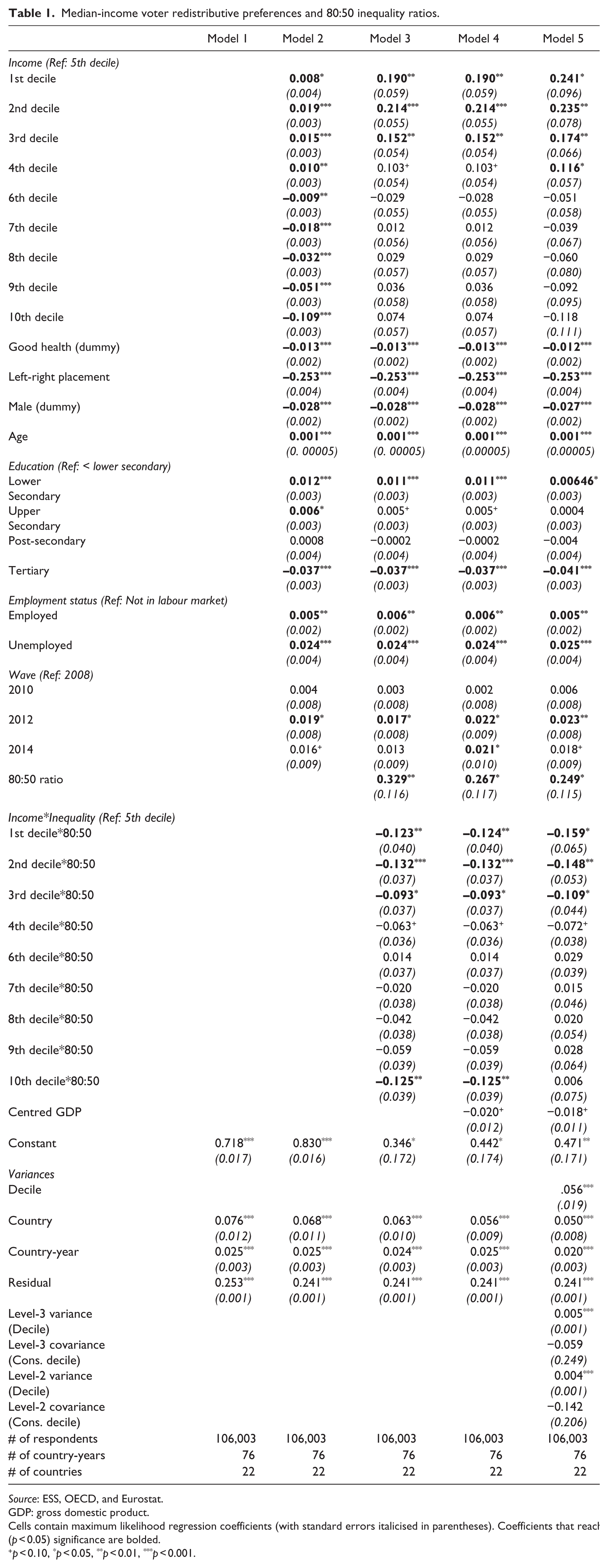
Table 1 presents our key findings in a step-wise fashion, homing in on the model featuring 80:50 inequality ratios: Model 1, the null model, is presented as a baseline; Model 2 adds the individual-level variables along with the survey wave dummies; Model 3 adds the inequality measure; Model 4 is the full (random-intercepts) model; and Model 5 incorporates random slopes for income deciles, both at the country and country-year level. We take this step-wise approach as a robustness check, as it provides some assurance that the results of the full model are not simply driven by a specific aspect of the model construction. The corresponding estimated variances are then included at the bottom of each column.

Table 1.

Median-income voter redistributive preferences and 80:50 inequality ratios.

	Model 1	Model 2	Model 3	Model 4	Model 5
Income (Ref: 5th decile)
1st decile		0.008^*	0.190^**	0.190^**	0.241^*
1st decile		(0.004)	(0.059)	(0.059)	(0.096)
2nd decile		0.019^***	0.214^***	0.214^***	0.235^**
2nd decile		(0.003)	(0.055)	(0.055)	(0.078)
3rd decile		0.015^***	0.152^**	0.152^**	0.174^**
3rd decile		(0.003)	(0.054)	(0.054)	(0.066)
4th decile		0.010^**	0.103⁺	0.103⁺	0.116^*
4th decile		(0.003)	(0.054)	(0.054)	(0.057)
6th decile		–0.009^**	−0.029	−0.028	−0.051
6th decile		(0.003)	(0.055)	(0.055)	(0.058)
7th decile		–0.018^***	0.012	0.012	−0.039
7th decile		(0.003)	(0.056)	(0.056)	(0.067)
8th decile		–0.032^***	0.029	0.029	−0.060
8th decile		(0.003)	(0.057)	(0.057)	(0.080)
9th decile		–0.051^***	0.036	0.036	−0.092
9th decile		(0.003)	(0.058)	(0.058)	(0.095)
10th decile		–0.109^***	0.074	0.074	−0.118
10th decile		(0.003)	(0.057)	(0.057)	(0.111)
Good health (dummy)		–0.013^***	–0.013^***	–0.013^***	–0.012^***
Good health (dummy)		(0.002)	(0.002)	(0.002)	(0.002)
Left-right placement		–0.253^***	–0.253^***	–0.253^***	–0.253^***
Left-right placement		(0.004)	(0.004)	(0.004)	(0.004)
Male (dummy)		–0.028^***	–0.028^***	–0.028^***	–0.027^***
Male (dummy)		(0.002)	(0.002)	(0.002)	(0.002)
Age		0.001^***	0.001^***	0.001^***	0.001^***
Age		(0. 00005)	(0. 00005)	(0.00005)	(0.00005)
Education (Ref: < lower secondary)
Lower		0.012^***	0.011^***	0.011^***	0.00646^*
Secondary		(0.003)	(0.003)	(0.003)	(0.003)
Upper		0.006^*	0.005⁺	0.005⁺	0.0004
Secondary		(0.003)	(0.003)	(0.003)	(0.003)
Post-secondary		0.0008	−0.0002	−0.0002	−0.004
		(0.004)	(0.004)	(0.004)	(0.004)
Tertiary		–0.037^***	–0.037^***	–0.037^***	–0.041^***
		(0.003)	(0.003)	(0.003)	(0.003)
Employment status (Ref: Not in labour market)
Employed		0.005^**	0.006^**	0.006^**	0.005^**
Employed		(0.002)	(0.002)	(0.002)	(0.002)
Unemployed		0.024^***	0.024^***	0.024^***	0.025^***
Unemployed		(0.004)	(0.004)	(0.004)	(0.004)
Wave (Ref: 2008)
2010		0.004	0.003	0.002	0.006
2010		(0.008)	(0.008)	(0.008)	(0.008)
2012		0.019^*	0.017^*	0.022^*	0.023^**
2012		(0.008)	(0.008)	(0.009)	(0.008)
2014		0.016⁺	0.013	0.021^*	0.018⁺
2014		(0.009)	(0.009)	(0.010)	(0.009)
80:50 ratio			0.329^**	0.267^*	0.249^*
80:50 ratio			(0.116)	(0.117)	(0.115)
IncomeInequality (Ref: 5th decile)*
1st decile*80:50			–0.123^**	–0.124^**	–0.159^*
1st decile*80:50			(0.040)	(0.040)	(0.065)
2nd decile*80:50			–0.132^***	–0.132^***	–0.148^**
2nd decile*80:50			(0.037)	(0.037)	(0.053)
3rd decile*80:50			–0.093^*	–0.093^*	–0.109^*
3rd decile*80:50			(0.037)	(0.037)	(0.044)
4th decile*80:50			−0.063⁺	−0.063⁺	−0.072⁺
4th decile*80:50			(0.036)	(0.036)	(0.038)
6th decile*80:50			0.014	0.014	0.029
6th decile*80:50			(0.037)	(0.037)	(0.039)
7th decile*80:50			−0.020	−0.020	0.015
7th decile*80:50			(0.038)	(0.038)	(0.046)
8th decile*80:50			−0.042	−0.042	0.020
8th decile*80:50			(0.038)	(0.038)	(0.054)
9th decile*80:50			−0.059	−0.059	0.028
9th decile*80:50			(0.039)	(0.039)	(0.064)
10th decile*80:50			–0.125^**	–0.125^**	0.006
10th decile*80:50			(0.039)	(0.039)	(0.075)
Centred GDP				−0.020⁺	−0.018⁺
Centred GDP				(0.012)	(0.011)
Constant	0.718^***	0.830^***	0.346^*	0.442^*	0.471^**
Constant	(0.017)	(0.016)	(0.172)	(0.174)	(0.171)
Variances
Decile					.056^***
Decile					(.019)
Country	0.076^***	0.068^***	0.063^***	0.056^***	0.050^***
Country	(0.012)	(0.011)	(0.010)	(0.009)	(0.008)
Country-year	0.025^***	0.025^***	0.024^***	0.025^***	0.020^***
Country-year	(0.003)	(0.003)	(0.003)	(0.003)	(0.003)
Residual	0.253^***	0.241^***	0.241^***	0.241^***	0.241^***
Residual	(0.001)	(0.001)	(0.001)	(0.001)	(0.001)
Level-3 variance					0.005^***
(Decile)					(0.001)
Level-3 covariance					−0.059
(Cons. decile)					(0.249)
Level-2 variance					0.004^***
(Decile)					(0.001)
Level-2 covariance					−0.142
(Cons. decile)					(0.206)
# of respondents	106,003	106,003	106,003	106,003	106,003
# of country-years	76	76	76	76	76
# of countries	22	22	22	22	22

Source: ESS, OECD, and Eurostat.

GDP: gross domestic product.

Cells contain maximum likelihood regression coefficients (with standard errors italicised in parentheses). Coefficients that reach (p < 0.05) significance are bolded.

p < 0.10, ^*p < 0.05, ^**p < 0.01, ^***p < 0.001.

Results across the models are overall quite consistent. Addressing the control variables first, the standard individual-level variables have the expected effects. Youth, higher education levels, and right-wing self-placement are all associated with lower preferences for redistribution, as is being male and being in good health. Relative to those not in the labour market, unemployed persons are notably more likely to support redistribution, while employed persons are marginally more likely. At the national level, the positive effect of GDP nears significance, which is not a trivial result given the relatively limited number of countries in our sample.

Most importantly, we find that higher 80:50 inequality ratios are associated with increased preferences for redistribution among middle-income groups – specifically among the fifth and sixth deciles, though this only becomes clear once we incorporate the standard robustness checks. Since we are interested in an interaction effect, the key results in Table 1 should be read carefully: coefficients for the direct and interaction effects between inequality and decile grouping are relative not only to one another, but also to the fifth income decile, which we set as the baseline group given the apparent importance of the middle-income groups in this analysis. This makes it very difficult to assess specific findings in isolation. To address this complexity, Figure 2 presents the average marginal effects of the 80:50 inequality ratio across the income decile groups. The top panel presents the results from the random-intercepts only model (Model 4), while the bottom illustrates the effect once we allow the effect of income deciles to vary across countries and country-years (Model 5).

Figure 2.

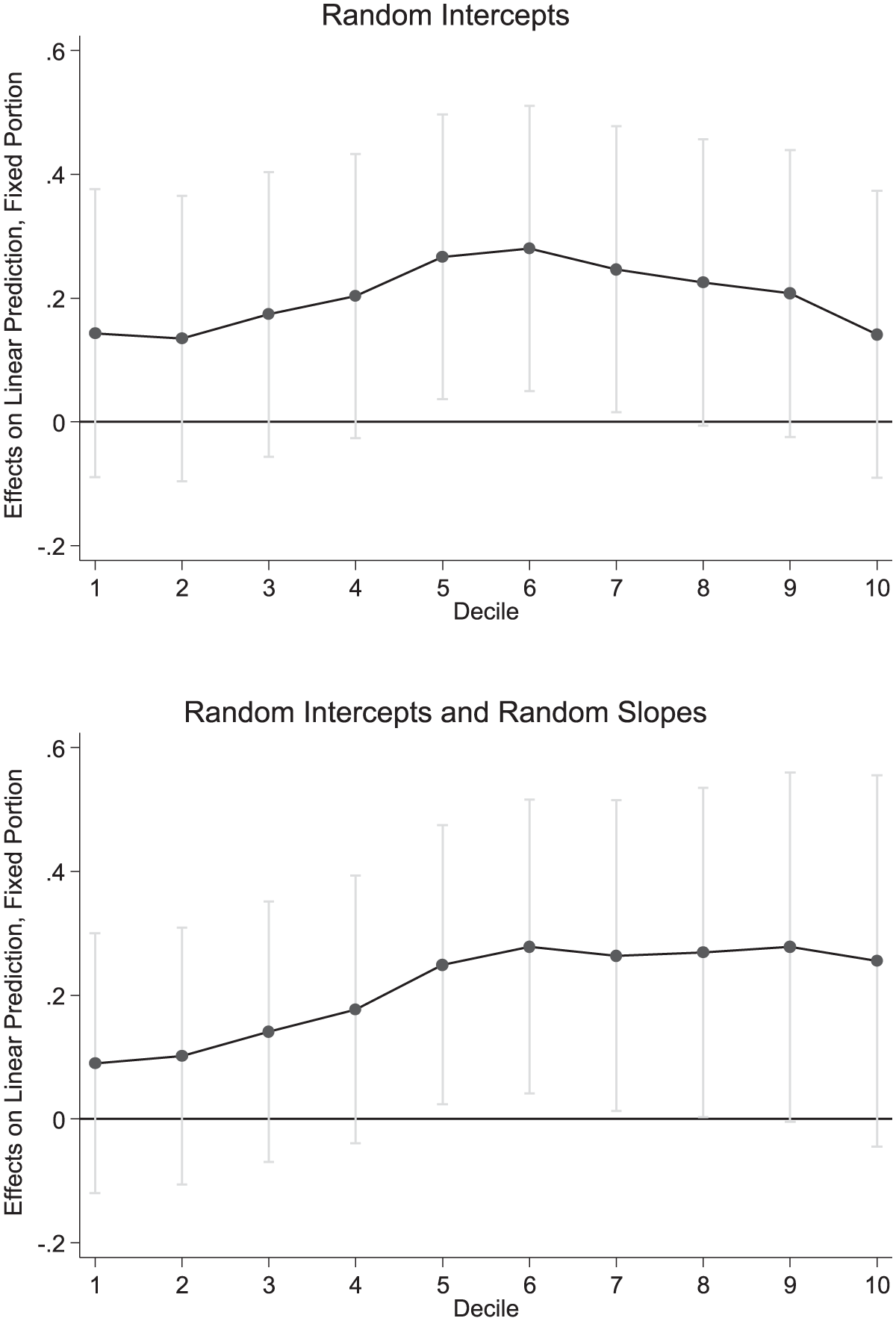
Average marginal effects of 80:50 ratio with 95 percent CIs.

Turning first to the top panel of Figure 2, initial results suggest that it is among the fifth, sixth, and seventh decile groups that the 80:50 inequality ratio appears to make a difference. These findings indicate that, for these groups, moving from the lowest to the highest inequality country would be associated with an increased preference for redistribution of about 0.09. This is a greater difference than that found across the interquartile range of country-mean redistributive preferences – that is, comparing the mean response in the Czech Republic (at 0.67) to that in Finland (at 0.74). And while increases related to the 80:50 inequality ratio could only account for a limited portion of overall variation (with responses to the question ranging from 0 to 1 and exhibiting a standard deviation of 0.26), the effect is larger than those correlated with standard variables in the literature, such as unemployment (at slightly under 0.03), being in good health (at 0.01), and education (at 0.04 across the full range of levels). Age and ideology are the only control variables that might potentially have a larger effect – but even with them moving across the inter-quartile ranges is correlated with shifts of 0.03 and 0.08, respectively.

While at first these effects appear to extend from the fifth through to the seventh decile, additional analysis confirms that they are robust only for the fifth and sixth decile. The standard robustness checks were carried out in four stages (with the effect of the 80:50 inequality ratio on the seventh frequently failing to reach significance). First, in the bottom panel of Figure 2, we noted similar results when we allowed the effect of income deciles to differ across countries and country-years (using random slopes). As discussed above, this provides some safeguard that unaccounted-for heterogeneity is not driving our main effects. Second, we confirmed that the results are robust to various alterations to the model specification: we do so, most notably, by changing the variables included in the model⁷ and removing Israel from the sample (given the atypically high imbalance in the distribution of respondents across the income distribution). Third, we reran the analysis using country robust standard errors, finding that the effects only remain significant for the fifth and sixth decile groups (see Figure 3). Finally, we re-ran the model 22 times, excluding one country at a time (i.e. remove-one jackknife) to confirm that our results are not driven entirely by a single case. Here again, the interaction effects are only consistent for the fifth and sixth decile groups; with largely equivalent, though slightly larger coefficients, their p-values both remain below 0.1 (see Figure 4).

Overall, the results demonstrate that the structure of inequality is worthy of detailed attention. Although many scholars have debated whether higher levels of general inequality, as measured by the Gini coefficient, are associated with increased median-voter preferences for redistribution, this discussion can only take us so far. Looking at a wide variety of inequality ratios, we find that (1) the structure of inequality only has a robust effect on middle-income groups – specifically the fifth and sixth decile groups and (2) it is only one specific type of inequality that appears to matter – that between middle income groups and those around the 80th percentile. This leads us to tentatively find greater support for the Envy your Brother hypothesis over the Soak the Rich hypothesis. Nevertheless, we cannot rule out a potential effect of data quality issues at the extreme ends of the income distribution, and this distinction therefore clearly warrants further research.

Conclusion

In this article, we have explored how the structure of inequality affects the redistributive preferences of citizens across the income distribution. Somewhat unexpectedly, much of the action is in fact related to the politically interesting median-income group: although we examined the determinants of preferences across the income distribution, the empirical results suggest that it is only within the middle-income groups that the structure of inequality has an effect. For all decile groups but the fifth and the sixth, we found no robust effects of inequality.

Given that the median-income voter is often thought to wield a lot of influence over who gets elected and what social policies are pursued (e.g. Iversen and Soskice, 2006; Jensen, 2012; Tepe and Vanhuysse, 2009), our findings speak to a broad body of literature. Contrary to theories based on the Social Rivalry, Insurance, or Social Affinity hypotheses, as well as the findings of Tóth and Keller (2014), the distance to the bottom does not affect the median income groups’ preferences for redistribution. What matters for the median-income segment is the distance to those with more resources than themselves. In particular, it is the distance to what one might think of as the ‘upper-middle class’ – the well-off-but-not-rich – that is associated with greater median-income segment support for redistribution. Although individuals often have a difficult time assessing the overall extent of inequality in their societies (e.g. Kenworthy and McCall, 2008; McCall, 2013; Norton and Ariely, 2011), this appears to be one form of inequality that bucks the trend.

The interpretation of the relationship appears reasonably straightforward: the inequality between the median-income segment and those around the 80th percentile is highly visible for members of the median-income segment because of the comparably similar lifestyles that the two groups tend to live. More research will be needed to assess the mechanisms underlying this relationship, however, as the present study does not allow us to examine how middle-income groups become aware of increased inequality. Studies on the consequences of geographic proximity and/or shared workplaces would be particularly valuable in this regard. Relatedly, the potential effect of class distinctions between the 50th and 80th percentiles is also of interest: an investigation into the consequences of middle- versus upper-middle class markers therefore offers another route forward. Middle-class attitudes towards the upper-middle class may differ in crucial ways from those towards the very rich, in particular as they relate to hopes of upwards social mobility.

In addition, the present study is also unable to ascertain whether middle-income group preferences for redistribution are primarily self-serving (with an interest only in redistribution towards the middle class) or also contain a substantial other-regarding component (perhaps due to a concern with inequality per se). Future work will thus especially benefit from survey data that disaggregate redistributive preferences along self- and other-oriented dimensions (see Cavaillé and Trump, 2015). And while we can say fairly confidently that the distance between the median income segment and the bottom does not matter and that the distance to the top does, we are less certain that it really is the distance to the upper middle class rather than the rich that matters. Although the 80:50 model points to the most robust effect of inequality on middle-income attitudes, it remains difficult to confidently capture data on the very highest incomes. The statistical results presented here should therefore be supplemented with additional studies in the future in order to reach a firmer conclusion on this point. In particular, we envision that more focused surveys, perhaps including survey experiments, might be able to more precisely inform us about the yardsticks of inequality used when forming opinions about redistribution.

More broadly, our results should be read in conjuncture with research on the relationship between class differences and redistributive preferences (e.g. Edlund and Lindh, 2015; Kumlin and Svallfors, 2007; Svallfors, 2006). We therefore believe that future research that exports the analytical framework presented here to issues of class relations and class identities would be particularly fruitful for assessing the effects of the structure of inequality on redistributive preferences.

Footnotes

Appendix 1

Table 3.

Descriptive statistics of all variables (note that there are 106,003 observations for each variable.).

Variable	Mean	Standard deviation	Min	Max
Preference for redistribution	0.704	(0.264)	0	1
Income decile	5.446	(2.755)	1	10
Good health (dummy)	0.679	(0.467)	0	1
Left–right self-placement	0.508	(0.215)	0	1
Male (dummy)	0.491	(0.500)	0	1
Age	49.164	(17.841)	14	123
Education	3.285	(1.334)	1	5
Employed (dummy)	0.524	(0.499)	0	1
Unemployed (dummy)	0.041	(0.198)	0	1
ESS Round	5.486	(1.098)	4	7
80:50 Ratio	1.472	(0.087)	1.335	1.688
Centred GDP	0.490	(1.006)	−1.594	3.237

GDP: gross domestic product; ESS: European Social Survey.

Funding

The author(s) received no financial support for the research, authorship, and/or publication of this article.

Notes

References

Alt

Iversen

(2017) ‘Inequality, Labor Market Segmentation and Preferences for Redistribution’, American Journal of Political Science 61(1): 21–36.

Andrews

Leigh

(2009) ‘More Inequality, Less Social Mobility’, Applied Economics Letters 16(15): 1489–92.

Barth

Finseraas

Moene

K.O.

(2015) ‘Political Reinforcement: How Rising Inequality Curbs Manifested Welfare Generosity’, American Journal of Political Science 59(3): 565–77.

Benabou

(2000) ‘Unequal Societies: Income Distribution and the Social Contract’, American Economic Review 90(1): 96–129.

Bonica

McCarty

Poole

K.T.

Rosenthal

(2013) ‘Why Hasn’t Democracy Slowed Rising Inequality?’, Journal of Economic Perspectives 27(3): 103–23.

Bradley

Huber

Moller

Nielsen

Stephens

J.D.

(2003) ‘Distribution and Redistribution in Postindustrial Democracies’, World Politics 55(2): 193–228.

Cavaillé

Trump

K.-S.

(2015) ‘The Two Facets of Social Policy Preferences’, Journal of Politics 77(1): 146–60.

Corneo

Grüner

H.P.

(2000) ‘Social Limits to Redistribution’, American Economic Review 90(5): 1491–507.

Cusack

Iversen

Rehm

(2006) ‘Risks at Work: The Demand and Supply Sides of Government Redistribution’, Oxford Review of Economic Policy 22(3): 365–89.

10.

Dallinger

(2010) ‘Public Support for Redistribution: What Explains Cross-National Differences?’, Journal of European Social Policy 20(4): 333–49.

11.

Dallinger

(2015) ‘Public Redistribution and Voter Demand: The Role of the Middle Class’, Comparative Sociology 14(6): 721–50.

12.

Druckman

J.N.

(2014) ‘Pathologies of Studying Public Opinion, Political Communication and Democratic Responsiveness’, Political Communication 31(3): 467–92.

13.

Edlund

Lindh

(2015) ‘The Democratic Class Struggle Revisited: The Welfare State, Social Cohesion and Political Conflict’, Acta Sociologica 58(4): 311–28.

14.

Eurostat (2010) An Assessment of Survey Errors in EU-SILC. Luxembourg: Eurostat Publications Office.

15.

Finseraas

(2009) ‘Income Inequality and Demand for Redistribution: A Multilevel Analysis of European Public Opinion’, Scandinavian Political Studies 32(1): 94–119.

16.

Fischer

C.S.

Stockmayer

Stiles

Hout

(2004) ‘Distinguishing the Geographic Levels and Social Dimensions of US Metropolitan Segregation, 1960–2000’, Demography 41(1): 37–59.

17.

Hacker

J.S.

Pierson

(2011) Winner-Take-All Politics: How Washington Made the Rich Richer – and Turned Its Back on the Middle Class. New York: Simon & Schuster.

18.

Iversen

Soskice

(2006) ‘Electoral Institutions and the Politics of Coalitions: Why Some Democracies Redistribute More Than Others’, American Political Science Review 100(2): 165–81.

19.

Jæger

M.M.

(2006) ‘What Makes People Support Public Responsibility for Welfare Provision: Self-Interest or Political Ideology? A Longitudinal Approach’, Acta Sociologica 49(3): 321–38.

20.

Jæger

M.M.

(2013) ‘The Effect of Macroeconomic and Social Conditions on the Demand for Redistribution: A Pseudo Panel Approach’, Journal of European Social Policy 23(2): 149–63.

21.

Jensen

(2012) ‘Labour Versus Life Course-Related Social Policies: Understanding Cross-Programme Differences’, Journal of European Public Policy 19(2): 275–91.

22.

Kelly

N.J.

Enns

P.K.

(2010) ‘Inequality and the Dynamics of Public Opinion: The Self-Reinforcing Link between Economic Inequality and Mass Preferences’, American Journal of Political Science 54(4): 855–70.

23.

Kenworthy

McCall

(2008) ‘Inequality, Public Opinion and Redistribution’, Socio-economic Review 6(1): 35–68.

24.

Kenworthy

Pontusson

(2005) ‘Rising Inequality and the Politics of Redistribution in Affluent Countries’, Perspectives on Politics 3(3): 449–71.

25.

Kumlin

Svallfors

(2007) ‘Social Stratification and Political Articulation: Why Attitudinal Class Differences Vary across Countries’, in Mau

Veghte

(eds) Social Justice, Legitimacy and the Welfare State, pp. 19–46. Aldershot: Ashgate.

26.

Lübker

(2007) ‘Inequality and the Demand for Redistribution: Are the Assumptions of the New Growth Theory Valid?’, Socio-Economic Review 5(1): 117–48.

27.

Lupu

Pontusson

(2011) ‘The Structure of Inequality and the Politics of Redistribution’, American Political Science Review 105(2): 316–36.

28.

Luttig

(2013) ‘The Structure of Inequality and Americans’ Attitudes toward Redistribution’, Public Opinion Quarterly 77(3): 811–21.

29.

McCall

(2013) The Undeserving Rich: American Beliefs about Inequality, Opportunity and Redistribution. Cambridge: Cambridge University Press.

30.

McCall

Chin

(2013) ‘Does Knowledge of Inequality Affect Beliefs about Inequality’, Midwest Political Science Association Conference, Chicago, IL, 11–14 April.

31.

Matthijs

(2016) ‘The Euro’s ‘Winner-Take Political Economy: Institutional Choices, Policy Drift and Diverging Patterns of Inequality’, Politics & Society 44(3): 393–422.

32.

Meltzer

A.H.

Richard

S.F.

(1981) ‘A Rational Theory of the Size of Government’, Journal of Political Economy 89(5): 914–27.

33.

Milanovic

(2000) ‘The Median-Voter Hypothesis, Income Inequality and Income Redistribution: An Empirical Test with the Required Data’, European Journal of Political Economy 16(3): 367–410.

34.

Moene

K.O.

Wallerstein

(2001) ‘Inequality, Social Insurance and Redistribution’, American Political Science Review 95(4): 859–74.

35.

Norton

M.I.

Ariely

(2011) ‘Building a Better America – One Wealth Quintile at a Time’, Perspectives on Psychological Science 6(1): 9–12.

36.

O’Brien

(2007) ‘A Caution Regarding Rules of Thumb for Variance Inflation Factors’, Quality & Quantity 41(5): 673–90.

37.

Page

B.I.

Bartels

L.M.

Seawright

(2013) ‘Democracy and the Policy Preferences of Wealthy Americans’, Perspectives on Politics 11(1): 51–73.

38.

Rehm

Hacker

J.S.

Schlesinger

(2012) ‘Insecure Alliances: Risk, Inequality and Support for the Welfare State’, American Political Science Review 106(2): 386–406.

39.

Rodríguez

(2004) ‘Inequality, Redistribution and Rent-Seeking’, Economics & Politics 16(3): 287–320.

40.

Romer

(1975) ‘Individual Welfare, Majority Voting and the Properties of a Linear Income Tax’, Journal of Public Economics 4(2): 163–85.

41.

Rueda

Stegmueller

(2016) ‘The Externalities of Inequality: Fear of Crime and Preferences for Redistribution in Western Europe’, American Journal of Political Science 60(2): 474–89.

42.

Schmidt-Catran

A.W.

(2016) ‘Economic Inequality and Public Demand for Redistribution: Combining Cross-Sectional and Longitudinal Evidence’, Socio-Economic Review 14(1): 119–40.

43.

Schmidt-Catran

A.W.

Fairbrother

(2016) ‘The Random Effects in Multilevel Models: Getting Them Wrong and Getting Them Right’, European Sociological Review 32(1): 23–38.

44.

Shapiro

(2002) ‘Why the Poor Don’t Soak the Rich’, Daedalus 131(1): 118–28.

45.

Soroka

S.N.

Wlezien

(2010) Degrees of Democracy: Politics, Public Opinion and Policy. New York: Cambridge University Press.

46.

Soroka

S.N.

Johnston

Kevins

Banting

Kymlicka

(2016) ‘Migration and Welfare State Spending’, European Political Science Review 8(2): 174–93.

47.

Steele

L.G.

(2015) ‘Income Inequality, Equal Opportunity and Attitudes about Redistribution’, Social Science Quarterly 96(2): 444–64.

48.

Svallfors

(2006) The Moral Economy of Class: Class and Attitudes in Comparative Perspective. Stanford, CA: Stanford University Press.

49.

Tepe

Vanhuysse

(2009) ‘Are Aging OECD Welfare States on the Path to Gerontocracy?’, Journal of Public Policy 29(1): 1–28.

50.

Tóth

I.G.

Keller

(2014) ‘Income Distribution, Inequality Perceptions and Redistributive Preferences in European Countries’, in Gornick

Jäntti

(eds) Income Inequality: Economic Disparities and the Middle Class in Affluent Countries, pp. 173–203. Stanford, CA: Stanford University Press.

51.

Trump

K.-S.

(2017) ‘Income Inequality Influences Perceptions of Legitimate Income Differences’, British Journal of Political Science (Early Access) 1–24.