A sclerochronological archive for Antarctic coastal waters based on the marine bivalve Yoldia eightsi (Jay,1839) from the South Orkney Islands

Abstract

The scarcity of long instrumental series from the Southern Ocean limits our understanding of key climate and environmental feedbacks within the Antarctic system. We present an assessment for the Antarctic mollusc bivalve Yoldia eightsi as an Antarctic coastal climatological archive, based on annually-resolved growth pattern of 20 live-collected specimens in 1988 from Factory Cove, Signy Island (South Orkney Islands). Two detrending methods were applied to the growth increment series: negative exponential detrending and regional curve standardization (RCS) detrending. The RCS-chronology showed consistent synchronous growth in the population for a 20 year period (1968-1988; expressed population signal ⩾ 0.85), a negative correlation between the RCS-chronology and the fast-ice duration record (r= -0.41, N= 24, P⩽ 0.05) and winter duration (r= -0.52, N=24, P⩽ 0.01) and positive correlations with mean winter sea surface temperature (SST; r= 0.57, N= 24, P⩽ 0.01), mean summer SST (r= 0.46, N= 24, P⩽ 0.05) and mean annual SST (r= 0.48, N= 24, P⩽ 0.05). The chronology appears to record the environmental conditions generated during the Weddell Polynya event (1973 -1976) as detectable abrupt changes in the annual growth patterns. Over eight years (1973-1980) a negative relationship between shell growth and suspended chlorophyll (i.e. a proxy for surface productivity) is apparent which is likely influenced by the seasonal deposition of organic phytodetritus on the seabed following surface water phytoplankton blooms. Our results form a basis for establishing Y. eightsi as an environmental archive for coastal Antarctic waters.

Keywords

Antarctica Signy Island Weddell Polynya marine proxy sclerochronology

Introduction

The Western Antarctic Peninsula is currently experiencing the fastest rates of climate warming (near surface air and ocean temperatures) in the Southern Hemisphere (e.g. Vaughan et al., 2003, 2013); an increase of 3°C in atmospheric temperature and an increase of 1°C in sea-surface temperature since 1951 have been reported (Meredith and King, 2005; Vaughan et al., 2013). This warming, linked to the southward movement of westerly air masses (Sokolov and Rintoul, 2009), impacting physical (sea-ice formation, ice-shelf stability, ice-stream dynamics) and biological systems with potentially significant environmental implications (e.g. for global sea levels). A full understanding of the mechanisms of this rapid change in the context of background natural variability, and of global and regional climate change, requires that the timing of the onset and subsequent evolution of the recent period of rapid warming be precisely determined. Constraining process rates in the Antarctic system is therefore of critical importance and such constraints require dating techniques applied to sedimentary and environmental archives that are both accurate and precise. In the Antarctic Peninsula region this is hampered by a relative lack of environmental proxies, especially in the marine realm, and those that do exist often rely on radiocarbon dating. For events and sequences covering the last 50,000 years, radiocarbon is widely used as the most suitable dating method available. However, the use of radiocarbon in the Southern Ocean is compromised by uncertainty in the spatial and temporal calibration of the regional offset in the radiocarbon reservoir effect (ΔR) as a result of the upwelling of old deep-waters and the short residence time of surface waters (Hall et al., 2010). Measurement of known age living material collected from around Antarctica prior to nuclear weapons testing indicates a mean reservoir age of 1131±125 years (compilation in Hall et al., 2010); ‘this presents a severe limitation when comparing the timing of past changes in circulation, climate, and ice-sheet dynamics in the Antarctic and Southern Ocean with those in other regions’ (Hall et al., 2010).

There is therefore an urgent need to identify Antarctic marine environmental archives that contain an annually-resolved structure similar to the terrestrial ice core record that can be precisely dated independently of their radiocarbon content. The use of annual growth increments in the shells of long-lived marine bivalves (e.g. Arctica islandica, Glycymeris glycymeris, Panopea generosa) to provide long, annually-resolved and absolutely-dated records of marine climate has become well established in recent years (e.g. Jones et al., 1989; Witbaard et al., 1997; Marchitto et al., 2000; Butler et al., 2009a, 2012; Reynolds et al., 2013). Growth increment series from living specimens can be cross-matched with similar overlapping series from dead-collected shells to generate statistically robust master chronologies (e.g. Marchitto et al., 2000; Schöne, 2003; Scourse et al., 2006; Reynolds et al., 2013). Variability in the chronology indices expresses the common environmental signal in the population (Wigley at al., 1986). In settings where instrumental series are available, growth increment variability is often correlated with climate variables (e.g. Jones et al., 1989; Schöne, 2003; Black et al., 2009; Butler et al., 2010; Brey et al., 2011; Reynolds et al., 2013) and can therefore be used for climate reconstruction. It is also possible to generate additional proxies of marine variables (such as seawater temperature, salinity and to quantify the marine radiocarbon reservoir) by calculating the δ¹⁸O, δ¹³C ratios and measuring ¹⁴C and trace element (e.g. Sr, Mn, Mg, Li) compositions of the carbonate forming the shell increments (e.g. Witbaard et al., 1994; Brey and Mackensen, 1997; Butler et al., 2009b; Freitas et al., 2012; Wanamaker et al., 2012; Cook et al., 2015). A sclerochronological study based on the Antarctic bivalve Laternula elliptica (King and Broderip, 1832) showed a close coupling between shell growth and regional climate variability modulated by El-Niño-Southern-Oscillation(Brey et al., 2011). We have therefore undertaken an investigation of the infaunal bivalve mollusc Yoldia eightsi (Jay, 1839) with a view to constructing annually-resolved sclerochronological archives of recent environmental change in the Antarctic.

Y. eightsi is widely distributed around Antarctica to depths of ~ 800 m (i.e. below significant ice scour depth), ranging from Tierra del Fuego, the Falkland Islands and southern Chile to circumpolar waters (Nolan and Clarke, 1993). It is most commonly found in the upper 2-3 cm of sediment in water depths down to 100 m depth (Dell, 1990). Similarly to other nuculanid species, Y. eightsi can function both as a suspension and as a deposit feeder and is able to change its feeding behaviour depending on the concentration of suspended organic particulate matter available in the surrounding water or on the seabed (Davenport, 1988; Abele et al., 2001). Peck and Bullough (1993) determined the length of the Y. eightsi growing season for adult specimens was approximately five months (mid-November to early April) using samples from Factory Cove (collected between February and April; see also Peck et al., 2000). Although suspension feeding is believed to occur throughout the year, this only seems to be energetically profitable during the short seasonal phytoplankton blooms (Davenport, 1988). The year round availability of suspended and deposited food lends support to the observation by Peck et al. (2000) that, in young (<5 years) Y. eightsi, growth is continuous throughout the year in Factory Cove, Signy Island (Figure 1), the same site as the present study. However shell growth was significantly reduced or even ceased in older individuals (>27 mm in length) during the Austral winter season (Peck et al., 2000). Similarly to Peck et al. (2000), Nakaoka and Matsui (1994) found a significant correlation (r= 0.75 ± 0.05 SD; P< 0.05; in specimens between two and eight ontogenetic years) between shell growth of the close related species Yoldia notabilis and the concentration of chlorophyll a in north-eastern Japan.

Figure 1.

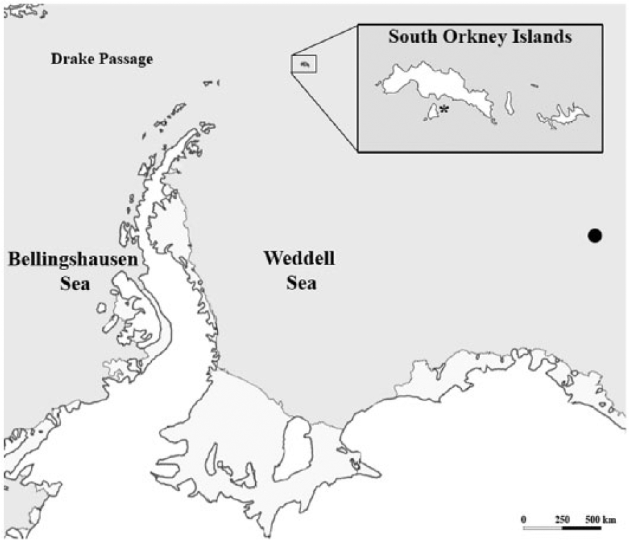
Map of the Atlantic sector surrounding Antarctica.The location of the BAS station at Signy Island, South Orkney Islands (Factory Cove, 67° 34′S, 68° 08′W) is indicated in the inset with an asterisk. The black dot indicates the location of the Maud Rise. A scale bar is also provided.

Nolan and Clarke (1993) reported distinct growth increment pattern from Y. eightsi shell sections which they assumed to be deposited annually.. Estimates of the longevity of Y. eightsi differ considerably depending on the method used. For example, Rabarts (1970), using external check marks on the shell surface, estimated the maximum age of Y. eightsi to be 19 years. However Davenport (1989) and later Peck and Bullough (1993), using catch-and-release techniques and Nolan and Clarke, (1993) employing ⁴⁵Ca incorporation into the mineralising shell, estimated a much longer life span of >60 years.

Yoldia eightsi has the potential to be a useful environmental / climatic archive for shallow Antarctic waters. The relatively high maximum longevity of Y. eightsi (>60 years; Davenport, 1989; Peck and Bullogough, 1993; Nolan and Clarke, 1993) when compared with L. elliptica (up to 40 years; Philipp et al., 2005) potentially allows the construction of longer chronologies. In addition, the extended depth distribution of Y. eightsi (up to 100m water depth; Dell, 1990) compared to the shallower habitat of L. elliptica (up to 30m water depth; Mercury et al., 1998) allows the investigation of deeper oceanographic processes. Yoldia eightsi also inhabits a shallower layer within the seabed (2-3cms; Dell, 1990) compared with L. elliptica (50cm; Mercury et al., 1998), facilitating the interpretation of geochemical proxies as traces of hydrographic conditions. Finally, the addition of a new sclerochronological record for the Antarctic will permit interspecies comparisons and facilitate calibrations of environmental proxies betweenspecies.

In this paper we examine growth increments from multiple specimens of Y. eightsi collected from Factory Cove, Signy Island (South Orkney Islands) and build the first shell-based chronology for this species. In addition, the relationships between environmental variables (including fast-ice duration, sea surface temperature (SST) and phytoplankton bloom activity) and the chronology are analysed and discussed.

Materials, methods and instrumental series

Sample collection

One hundred and seventy four specimens of Y. eightsi were live-collected in 1988 by British Antarctic Survey (BAS) SCUBA divers from depths <8m in Factory Cove, Signy Island, South Orkney Islands (60°43′S, 45°36′W, Figure 1). Twenty one individuals were live-collected in March, 112 during April, 10 in August and 31 in November 1988. Following collection the flesh was removed and the shell valves were air-dried and curated as individual disarticulated valves. The shell collection was then subsampled by shell length in order to target the longest-lived specimens and a total of 45 left valves were selected, comprising 11 valves from March, 17 valves from April, 8 valves from August and 9 valves from November. This spread of sampling months enabled an investigation into the seasonal timing of growth increment and growth line formation and seasonal changes in growth rate in Y. eightsi.

Sample preparation

The selected valves were embedded in epoxy resin and alongside the maximum growth axis (i.e. from umbo to ventral margin) using an IsoMet^® 5000 (Buehler^®) precision saw. Blade feeding rate during cutting was kept to 5 mm min^-1 to avoid damaging the fragile shells. The sectioned resin blocks were ground using progressively finer grades of carborundum paper (P400, P1200 and P1200/4000) and polished using diamond polishing paste (3 µm Ø). Exposed polished shell surfaces were etched for 30 min in 0.01 M HCl and acetate peels (0.35 µm thick acetate sheet) were prepared using the method described in Richardson (2001). Acetate peel replicas were mounted on microscope slides and observed under a transmitted light microscope. High resolution images of the peel replicas were photographed at x10 and x20 magnification using a camera attached to a microscope. The image analysis computer package OmniMet^© 9.5 (Buehler) was used to generate photomontages of the shell growth patterns in the ventral margin for subsequent measurement. The timing of formation of the last-deposited and partly-formed growth increment observed in the acetate peels was assessed by measuring the distance between the last marginal increment and the growth margin (marginal increment analysis (MIA). Growth increments were measured along the separation between the periostracum and the carbonate part of the shell from the ventral margin towards the umbo (Figure 2(a) and (b)). In addition, based on a scrutiny of the peel replicas, growth increments in Y. eightsi appear to be formed of a light portion, followed by a dark portion adjacent to the annually-formed growth lines (Figure 2(c)), this structural feature was also taken into consideration in the MIA.

Figure 2.

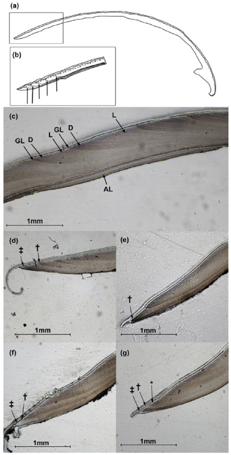
(a) Diagrammatic representation of a sectioned shell valve of Yoldia eightsi. (b) View of the shell margin to indicate the transect line (dashed-dotted line) where the incremental growth was measured. Growth lines are indicated by arrows. (c) Photomicrograph showing the growth pattern in a Y. eightsi peel. D: dark increments, L: light increments and GL: growth lines, AL: internal aragonitic layer. Scale and the exterior and interior sides are also shown. (d), (e), (f) and (g): Photomicrographs showing the characteristic marginal increments of Y. eightsi shells collected in: (d) March example, †: position of the previous year’s line. ‡: partial increment added during the summer (from November until March); note the hooked shape of the periostracum. (e) April example, †: recently formed current year’s line. (f) August example, †: current year’s line. ‡: light increment formed in winter (between April and August). (g) November example, †: light winter increment, ‡: increment produced during the current year’s summer, Asterisk: position of the previous year’s line. Scale bar (1 mm) is also shown.

Chronology development

To construct the growth increment series (GISs), the distance between consecutive annual growth lines was measured from the shell edge towards the umbo (Figure 2(a) and (b)). Subsequently, the 20 longest-lived specimens were selected for chronology development. Cross-matching between specimens was carried out using the program SHELLCORR (see Scourse et al., 2006). SHELLCORR displays the running correlations (Pearson correlation coefficients) between increment width series from two shells at consecutive temporal offsets or lags. The analysis identifies offsets and mismatches between two GISs by comparing high frequency variability in the GISs. The GISs were pre-whitened for cross-matching by applying a log function to the raw data and then applying a high-pass filter (15 year spline) to the data before normalizing (see Butler et al., 2010). GISs from each collection month were analysed separately in order to identify the best cross-match for each collection month as a reference for cross-matching. In addition, the best correlated pairs for each collection month were compared amongst each other in order to check for annual consistency. This is important due to the differential time in sampling; shell growth that occurred between the first and last collected specimens can potentially offset the GISs by one year.

The dendrochronological program ARSTAN v.41d (Cook and Krusic, 2007) was used to construct the sclerochronology and to determine the expressed population signal (EPS) values. The sclerochronology is constructed as a mean value function of the standardized growth indices (SGIs) of the individual detrended growth increment series (Butler et al., 2010). The EPS is a function of sample depth and the mean correlation between the series and represents the degree to which a particular chronology expresses the common growth signal in the population (Wigley et al., 1984). An EPS ranges between 0 and 1, with 1 being a perfect correlation between all cross-matched series. A value of 0.85 is conventionally considered to indicate a sufficiently robust common growth signal in the sample (Briffa and Jones, 1990). In environments with strong seasonal variability, such as Antarctica, the common variability in the chronologies is enhanced, and so a smaller number of series are required to achieve a high EPS (Mäkinen and Vanninen, 1999). To construct the chronology, the trend in variance in each growth increment series was first stabilised using an adaptive power transformation (Cook and Peters, 1997). Two chronologies were constructed using two different detrending methods to remove the ontogenetic growth trend: 1) the conventional application of a negative exponential (NE) function, i.e. NE-chronology (Butler et al., 2010) and 2) the construction of a regional curve based on ontogenetically aligned time series, i.e. RCS-chronology (Esper et al., 2003).The NE-chronology was developed using a bi-weight robust mean function of the growth increment series; the effect of this is to remove the influence of outliers (e.g. possible disturbance events caused by predators or ice scouring). The RCS-chronology was developed by first constructing a regional curve (i.e. the mean population growth series of the ontogenetically-aligned specimen growth series) and then subtracting it from the individual GISs. Pith-offset (PO) is the difference between the first year of growth and the first measurable year of growth and is a possible source of error in the development of a regional curve (Esper et al., 2003). No PO was calculated as shell abrasion at the umbo region due to Y. eightsi burrowing behaviour prevented an accurate estimation of missing increments. In addition, the effect of not calculating the PO is small when the PO is evenly distributed (Esper et al., 2003). Nonetheless, due to the similar shell sizes and similar umbo erosion among studied specimens the effect on PO error was considered minimal. EPS was calculated in both chronologies based on an 11 year window with a 10 year overlap.

Environmental data

Historical instrumental data including fast-ice duration (1947-2008) for Signy Island, archived at BAS (Murphy et al., 1995) and phytoplankton bloom intensity (mg Chl.m³) and duration (days) (Clarke et al., 1988) were compared with the chronologies. Fast-ice is defined as coastal sea-ice persisting fast to the coastline, an ice wall, an ice front or between grounded shoals that remains in position until the seasonal break out (Murphy et al., 1995). Fast-ice duration data (number of days between dates of break-out and formation) and number of ice-days data (total number of days for which fast-ice was present) were extracted from Murphy et al. (1995). Regional HadISST1 gridded data (http://www.metoffice.gov.uk/hadobs/hadisst/; 58-62°S, 43-47°W) from the MET Office Data Bank were used as an estimation of the inter-annual SST variations in the region. MET Office Data Bank data consists of global monthly median SST and sea-ice concentration values from 1870 to date at a spatial resolution of 1 degree latitude and longitude (Rayner et al., 2003). The HadISST1 data were filtered for the period concerning the chronology (1940-to date). The SST dataset was weighted by calculating linear correlations between the robust part of the RCS-chronology (EPS >0.85) and each calendar month, then monthly SST values were multiplied by the absolute monthly correlation coefficient. Subsequently annual (August-July), summer (November-June) and winter (July-October) SST arithmetic averages were calculated for the spatially and temporally filtered HadISST1 dataset. The selection of calendar months was undertaken by determining the month with the lowest SST value between 1964 and 1988 (i.e. August) for the mean annual SST; winter and summer months were selected with respect to the local temperature data published by Clarke et al. (1988). Summer months (November-June) include the main growing season of Y. eightsi, which was estimated to be five months long (Peck and Bullough, 1993; Nolan and Clarke, 1933). In order to determine the winter duration the monthly maximum, minimum and average of SST values between 1965 and 1988 were calculated and the first and second quartile (Q1 and Q2) of temperature values were determined. The number of days in calendar months with a temperature value below the Q1 and Q2 temperature values were pooled together in two separate datasets. The record with temperature values below Q1 was termed “core winter duration” and the record with temperature values below Q2 “extended winter duration”. Core winter duration and extended winter duration were compared against the developed chronologies. Intensity and duration of the phytoplankton bloom were combined into a single index, i.e. time integrated biomass (TIB) derived from a trapezoidal integration for the period between 1973 and 1980 (data extracted from: Clarke et al., 1988). High values of the TIB index represent relatively longer and stronger bloom conditions. SST, TIB and fast-ice duration datasets were tested for correlation (Pearson’s product-moment of correlation) with the chronologies, and the mean annual, mean winter and mean summer SST values were tested for correlation with the mean fast-ice duration using the programs SHELLCORR and SPSS v.16. Note that the SPSS correlation results coincide with SHELLCORR correlation results at 0-lag. A 15-year running correlation between the chronologies and the instrumental records was carried out in order to identify temporal changes in the relationships.

Results

Marginal growth increment analysis

The periostracum in the umbo region of large valves was worn away and damaged extending to the inner aragonite shell layer. This shell abrasion prevented the measurement of annually-formed increments during early life, between four and six years depending on the extent of abrasion (Román-González pers. obs.), of the specimens. The growth pattern in the outer aragonite layer appeared as a light region that gradually transitioned to a dark brown region that presented a narrow growth line at terminus (Figure 2(c)). In the mid-part of the shell this demarcation between light and dark regions was unclear because the dark brown colouration was smeared across the growth lines. Scrutiny of the sectioned shell margins of Y. eightsi collected at different times of the year showed that the growth line is likely deposited during April following formation of the increment during the Austral summer (see examples of photomicrographs of the shell margins in Figure 2(d) to (g).Valves collected in March (Figure 2(d)) consistently showed a wide dark brown increment at the margin preceded by a light increment. However in three out of 11 valves the final increment did not have a marked dark brown colouration, although a little colouration was present towards the inner surface at the margin of the shell. The greatest variability in the formation of the line occurred in the sections from the valves collected in April (Figure 2(e)). Seven out of 17 sections showed an apparent growth line right at the margin of the shell. The majority of April samples showed an obvious wide dark brown increment with no growth check and none showed a light increment at the terminus. Five out of eight sections from the valves collected in August (Figure 2(f)) displayed a narrow light increment at the shell margin followed by a brown increment. One section showed an apparent dark brown increment typical of the March specimens. The other two sections showed a brown increment in the penultimate position with a growth check; however the brown colouration was smeared right to the margin. Seven out of the nine November specimens (Figure 2(g)) showed a narrow brown increment right at the margin, presumably deposited during the beginning of the summer. The other two sections showed some discolouration beneath the periostracum and the previous light increment was partially fused with the last increment due to smearing of the brown colouration. In summary, annually-formed increments in Y. eightsi are formed of a light and dark portions that alternate throughout the growing season and present some degree of ontogenetic variability.

Chronology assessment

The construction of the chronologies (NE and RCS) for the Y. eightsi population was achieved using 20 longest-lived (19-41 years), measured and cross-matched left shell valves. Special preference was given to the RCS-chronology over the NE-chronology due to an ontogenetic growth rhythm overlapping the negative exponential growth trend in Y. eightsi (Román González et al. 2016). The regional curve, used in the development of the RCS-chronology, and the negative exponential detrending curve, used in the development of the NE-chronology, are shown in Figure 3. EPS values used to assess the robustness of the RCS-chronology are shown in Figure 4(a). Because of the running windows used for calculating the EPS, there are no EPS values between 1983 and 1988. Nonetheless this period showed strong synchronicity in shell growth among the individual specimens and is therefore included in the environmental analyses. The NE- and RCS-chronologies and the individual growth increments series are shown in Figure 4(b). The average lifespan of the specimens used in the chronology was 30 years of age; considering the 30 year period of 1959-1988 and that the EPS falls below the 0.85 threshold after 1968 it can be assumed that the fall of the EPS prior to 1968 is due to lack of correlation between the specimens (Figure 4(a)).

Figure 3.

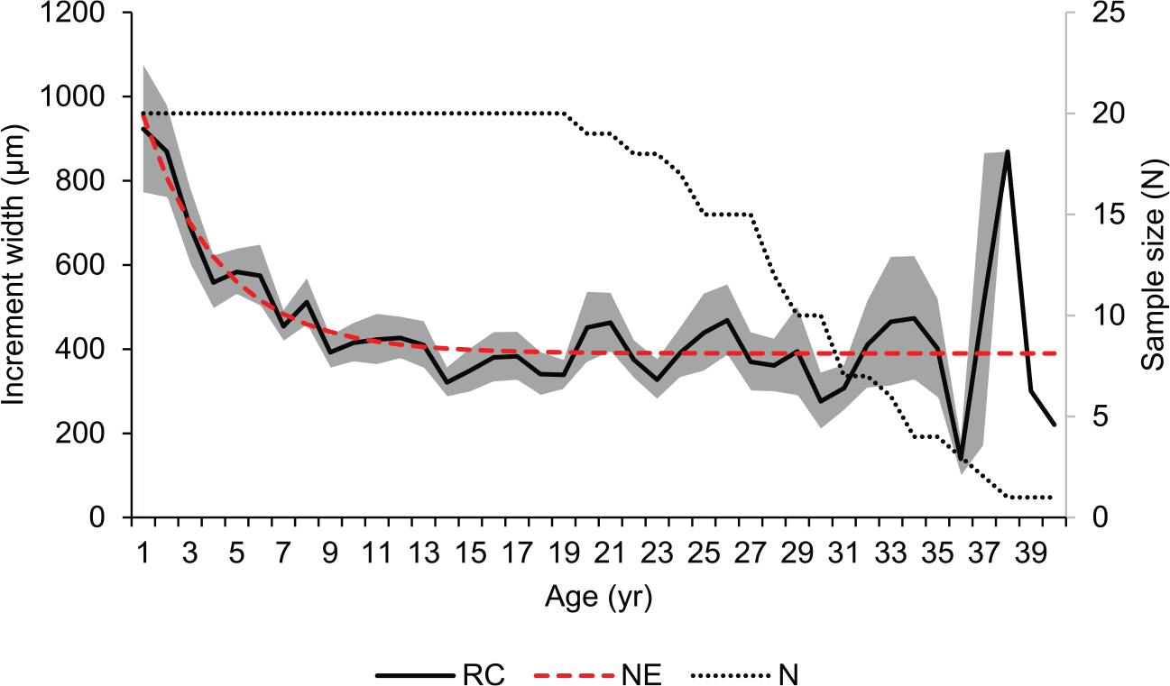
Regional curve (RC) of 20 Yoldia eightsi specimens (solid black) and the empirical negative (NE) exponential detrending curve (Y = 389.75 + 760.78 * e ^{(- 0.2995 * x)}, dashed red). Sample size (N) is also indicated with a dotted line. Standard error of the ontogenetic growth trend is indicated in the grey-shaded area.

Figure 4.

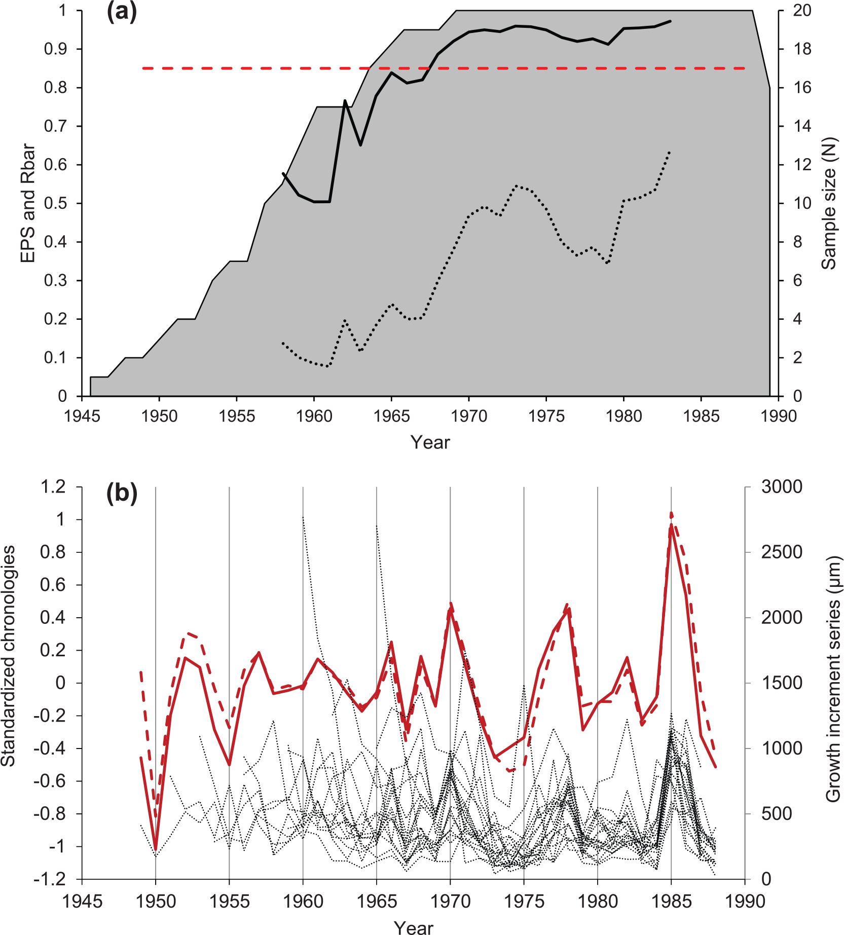
(a) Expressed population signal (EPS) (solid black) and Rbar values (i.e. mean correlation between all pairs of detrended; dotted black) calculated in an 11-year rolling window and 10-year overlap. EPS threshold of EPS=0.85 recommended by Wigley, et al. (1984) is shown in a dashed red line and sample size (i.e. number of individuals used to construct the chronology; grey shaded area). (b) Arstan RCS-chronology (solid red), Arstan NE-Chronology (dashed red) and the growth increment series of each specimen used in chronology construction (dotted lines).

The NE- and RCS-chronologies were compared with fast-ice duration, fast-ice cover and summer (November-June), winter (July-October) and mean annual (August-July) sea surface temperature (Table 1). The montly correlation coeffiecients calculated between 1963 and 1988 showed more positive correlations between April and November, except September, and weaker correlations between December and March (Jan 0.15, Feb 0.19, Mar 0.14, Apr 0.30, May 0.39, Jun 0.50, Jul 0.53, Aug 0.34, Sep 0.22, Oct 0.54, Nov 0.44, Dec −0.04). A negative correlation (r= −0.41, N= 24, P⩽ 0.05, R²= 0.17) was found between the RCS-chronology and fast-ice duration (Figure 5), whilst a negative correlation between fast-ice duration and mean annual SST was found (r= −0.43, N= 24, P⩽ 0.05) no correlation was apparent between the fast-ice duration and mean summer SST and mean winter SST between 1965 and 1988 (Table 1). SHELLCORR lagged correlation analysis showed an even stronger negative correlation at -1 lag between the RCS-chronology and fast-ice duration (r= -0.52) also positive correlation at +4 and -4 lags were highlighted (r= 0.58 and r= 0.51 respectively). In addition the RCS-chronology showed a positive correlation with mean winter SST values (r= 0.57, N= 24, P⩽ 0.01, R²= 0.33), with mean summer SST (r= 0.46, N= 24, P⩽ 0.05, R²= 0.21) and with the mean annual SST values (r= 0.48, N=24, P⩽ 0.05, R²= 0.23). The combination of both mean winter SST and fast-ice duration into a multiple regression significantly predicted the RCS-chronology, F(2,23)= 6.361, P⩽ 0.01, R²=0.377. A negative correlation between the RCS-chronology and core winter duration was found (r= -0.517, N= 24, P⩽ 0.01, R²= 0.27), although no correlation was found with extended winter duration. Similar values were obtained for the NE-chronology (Table 1) as there is a high similarity between both SGIs-chronologies (r= 0.92, N= 40, P⩽ 0.01, R²= 0.85). The SST data needs to be viewed with caution as the mean SST variability increases abruptly after 1972 (Figure 6); A 15-year window running correlation between the RCS-chronology and the fast-ice duration and summer and winter SST records is provided in Figure 7. A clear shift in correlation between the RCS-chronology and the SST datasets (from no correlation to positive) is obvious after 1972 (Figure 7). The relationship between the RCS-chronology and fast-ice duration remains negative for the entire length of the comparison (Figure 7). A negative relationship, although not significant, was observed between the TIB index and the RCS-chronology for a period of 8 years (1973-1980).

Table 1.

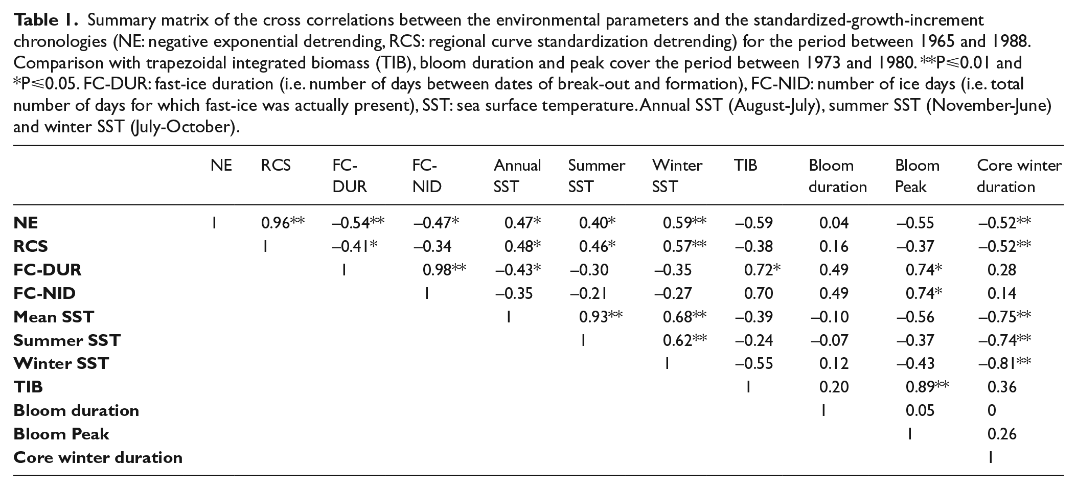
Summary matrix of the cross correlations between the environmental parameters and the standardized-growth-increment chronologies (NE: negative exponential detrending, RCS: regional curve standardization detrending) for the period between 1965 and 1988. Comparison with trapezoidal integrated biomass (TIB), bloom duration and peak cover the period between 1973 and 1980. **P⩽0.01 and *P⩽0.05. FC-DUR: fast-ice duration (i.e. number of days between dates of break-out and formation), FC-NID: number of ice days (i.e. total number of days for which fast-ice was actually present), SST: sea surface temperature. Annual SST (August-July), summer SST (November-June) and winter SST (July-October).

	NE	RCS	FC-DUR	FC-NID	Annual SST	Summer SST	Winter SST	TIB	Bloom duration	Bloom Peak	Core winter duration
NE	1	0.96**	−0.54**	−0.47*	0.47*	0.40*	0.59**	−0.59	0.04	−0.55	−0.52**
RCS		1	−0.41*	−0.34	0.48*	0.46*	0.57**	−0.38	0.16	−0.37	−0.52**
FC-DUR			1	0.98**	−0.43*	−0.30	−0.35	0.72*	0.49	0.74*	0.28
FC-NID				1	−0.35	−0.21	−0.27	0.70	0.49	0.74*	0.14
Mean SST					1	0.93**	0.68**	−0.39	−0.10	−0.56	−0.75**
Summer SST						1	0.62**	−0.24	−0.07	−0.37	−0.74**
Winter SST							1	−0.55	0.12	−0.43	−0.81**
TIB								1	0.20	0.89**	0.36
Bloom duration									1	0.05	0
Bloom Peak										1	0.26
Core winter duration											1

Figure 5.

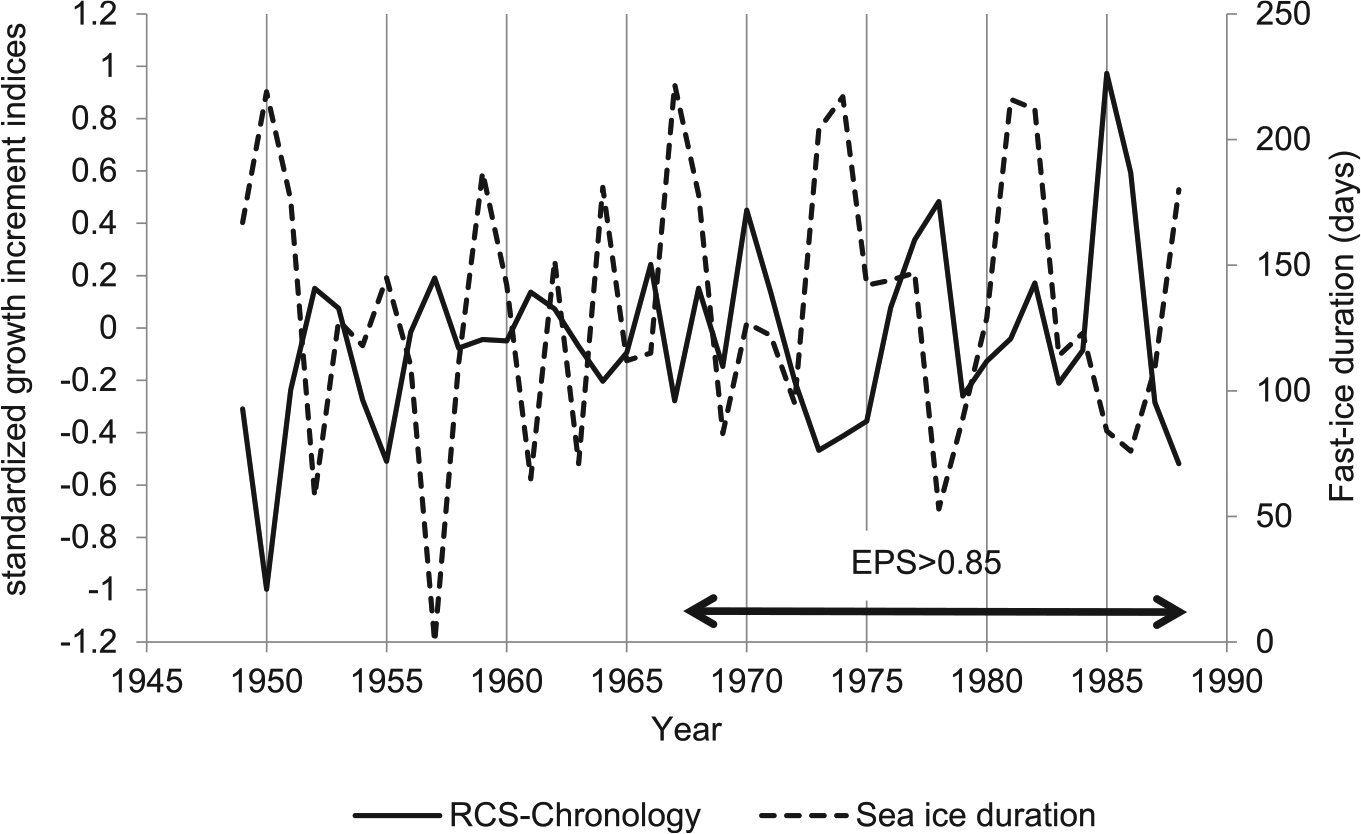
Standardized values for fast-ice duration (dashed line) and the regional-curve-standardization (RCS) chronology (solid line) between 1949 and 1988. The period with robust expressed population (EPS) signal is also indicated.

Figure 6.

Standardized growth increment indices (RCS-chronology, dashed line) and mean summer sea-surface temperatures (SST) (November-March, red shade, dark grey in monochrome), mean winter SST ((April-October), blue shade, light grey in monochrome) and mean annual SST (August-July, thin black line). The robust part of the RCS-chronology (Expressed population signal (EPS)>0.85) is shown with a double arrow.

Figure 7.

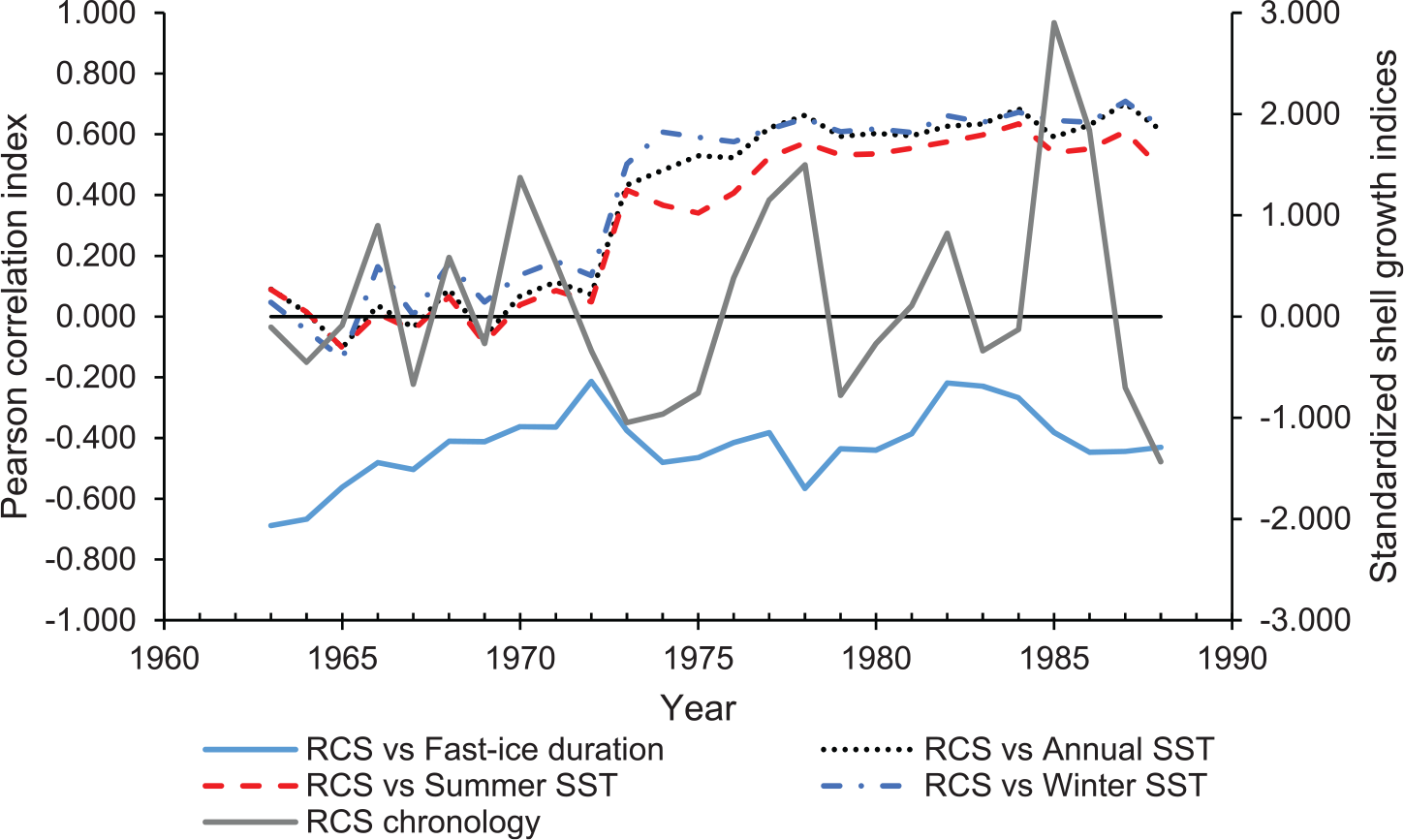
Running correlations (i.e. Pearson correlation index) in a 15-year window between the normalized Regional-Curve-Standardization (RCS) chronology (grey line) and fast-ice duration (solid blue line), mean annual sea surface temperatures (SST) (July-August, dotted black line), mean summer SST (November-June, dashed red line) and winter SST (July-October, dotted-dashed blue line) between 1963 and 1988. The solid black line indicates 0 correlation in the Pearson index.

The correlation analyses between the environmental parameters showed significant positive correlations between fast-ice duration and number of ice days (r= 0.98; N= 24, P⩽ 0.01, R²= 0.96) for the period 1949-1988 and TIB (r= 0.72, N= 8, P⩽ 0.05, R²= 0.51) and bloom peak (r= 0.74, N= 8, P⩽ 0.05, R²= 0.55) for the period 1973-1980; between mean annual SST and mean summer SST (r= 0.93, N= 24, P⩽ 0.01, R²= 0.86) and mean winter SST (r=0.68, N= 24, P⩽ 0.01, R²= 0.46) for the period 1965-1988; and between TIB and bloom peak (r= 0.89, N= 8, P⩽ 0.01, R²= 0.79) for the period 1973-1980. Strong negative correlations were found between core winter duration and mean annual SST (r= −0.75, N=24, P⩽ 0.01, R²= 0.56), summer SST (r= −0.74, N=24, P⩽ 0.01, R²= 0.54) and winter SST (r= −0.81, N=24, P⩽ 0.01, R²= 0.66). SHELLCORR lagged correlation analysis also showed a strong correlation, although less strong, between mean annual SST and mean winter SST at +1 and -1 year lag (r= 0.53 and r= 0.67 respectively). Additionally, mean summer SST and fast-ice duration showed a strong negative correlation at +5 lag (r= -0.63), mean winter SST and fast-ice duration showed a weak negative correlation at -2 lag (r= -0.38), A summary of the correlation analyses amongst the variables is provided in Table 1.

Discussion

Seasonality in the shell record

The colouration in the growth pattern of Y. eightsi appears to be similar to that in Y. notabilis reported by Nakaoka and Matsui (1994) (i.e. alternating light and dark regions within an annually-formed increment). The seasonal availability, quantity and quality of suspended and deposited organic material arising from phytoplankton blooms as well as the rate of shell-carbonate crystal formation may be important drivers for the formation of the different colouration in the wide increments and the development of a clear growth line following deposition of the summer increment (e.g. Lutz, 1976; Jones, 1980; Witbaard, 1996; Richardson, 2001). Some shells displayed a brown colouration that was present throughout the increments overlapping into adjacent increments. The greatest variability in the timing of formation of the growth line occurred in shell sections collected in April with only seven out of 17 shell sections showing a clear growth line right at the margin. April is the period of major seasonal changes in the Antarctic at the end of the Austral summer and appears to be a crucial month in the growth and physiology of Y. eightsi. April is also the month when suspension-feeding strategy acquires more importance in Y. eightsi physiology as a result of the increased dietary contribution from the phytoplankton bloom (Davenport, 1988). The MIA appears to contrast with the observations made by Peck et al. (2000) that growth in adult Y. eightsi individuals (>27 mm in length) was significantly reduced or even ceased during the Austral winter season. Yoldia eightsi growth tends to show positive correlations with organic matter concentration in sediments rather than suspended organic matter (Peck et al., 2000); there is a lack of correlation in the present study between the shell growth indices (NE-chronology and RCS-chronology) and the TIB, bloom peak and bloom duration parameters between 1965 and 1980 (Table 1). All specimens in our study were >27 mm (in length), however the MIA suggests some degree of shell growth throughout the year, albeit at a slower rate during the Austral winter months. Alternatively this period of shell growth may also have included a period of early spring shell growth. The skewed sampling distribution towards summer months and the lack of studies of microgrowth in the carbonate crystals of Y. eightsi prevents resolution with the conflicting results of Peck et al. (2000). Assessing the timing of the formation of the growth line is necessary when comparing a chronology with environmental records as it can result in a misalignment between both records.

The synchronous growth, controlled the environment, of Y. eightsi population at Factory Cove is reflected in the EPS (Figure 4(a)). The importance of this is that synchronous growth is necessary to produce chronologies that can be used to analyse long-term changes in the environment. The fall of EPS prior to 1968 was likely due to the lack of agreement in the growth increment series (Figure 4(a)). At this point in the chronology, the introduction of variability associated with vital effects in the early part of the growth increment series can decrease the strength of the correlation. This can be observed in the individual growth increment series in Figure 4(b) prior to 1968 where the lack of agreement between the series when compared to the period 1968-1988 is obvious.

Although the NE-chronology presents stronger correlations with the environmental parameters than the RCS-chronology (Table 1), an innate ontogenetic growth rhythm superimposed to the negative exponential growth trend was found in Y. eightsi (Román González et al. 2016) which is not accounted for by carrying out negative exponential detrending.

In addition fast-ice duration explains a significant amount of the phytoplankton bloom activity (R²= 0.52) compared to any of the SST datasets. This reinforces the notion that fast-ice duration is a major environmental driver at the coastal regions South Orkney Islands.

Environmental drivers of shell growth

The most prominent features in the chronology are increases in growth in 1970, 1977 and 1985, and a noticeable period of weak growth between 1973 and 1976 (Figure 4(b)). Between 1973 and 1976 a phenomenon known as the Weddell Polynya (WP) influenced the region, characterised by convective water circulation formed by surface salinity changes in the Weddell Sea (Gordon, 1982). Holland (2001) identified deep upwelling processes surrounding the Maud Rise seamount (Figure 1, 66°0′S, 3°0′E) as playing a major role in the development of the WP. Since the physical processes driving the formation of the WP altered the whole water column stratification, the decrease in mean annual SST observed at Signy Island was likely related to the same processes that formed the WP. Gordon (1982) reported the existence of a ‘cold spot’ under the sea surface, which migrated westwards (i.e. towards Signy Island) at an annual average drift rate of 1.3 cm.sec^-1. This suggests that ocean waters surrounding Signy Island could have been affected by this cold oceanographic regime. The satellite SST data indicates a pronounce decrease mean summer SST (1973) and mean winter SST (1973-1975; Figure 6). The RCS-chronology indices showed a sharp decline in shell growth between 1970 and 1973 that subsequently remained low for the period 1973-1976 (Figure 6). Additionally RCS-chronology indices show a period of fast growth between 1975 and 1977 which coincides with an increase in the mean annual SST due mainly to relatively warm temperatures during winter (Figure 6). Subsequently there is sharp decline in growth (1978-1979) that coincides with a decrease in mean annual SST that lasted until 1980. It is difficult to determine whether the Y. eightsi population at Signy Island responded to the effects of the cold conditions that originated in the WP before even the full development of the WP, as indicated by the sharp decline in growth between 1970 and 1973. The lack of quality winter SST data prior to 1973 (note the lack of variability in the mean winter SST values prior to 1973; Figure 6), prevents the determination of the onset of this cold regime. This indicates some degree of sensitivity of Y. eightsi to changes in SST, especially during winter season. Yoldia eightsi sensitivity to winter SST can be also detected in the monthly-calculated correlation coefficients with stronger positive correlations between April and November (except September) and weaker correlations during the summer (December-March). This suggests that another environmental parameter is controlling shell growth during summer months. It is very likely that deposited organic matter availability due to the phytoplankton bloom is the main environmental driver during the summer and as winter progresses and food availability becomes scarce, SST starts to play a more important role in regulating shell growth.

The SST data need to be viewed with caution as the mean SST values are based on oceanic SST values calculated from satellite measurements and the sparse instrumental data available (Figure 6; Rayner et al., 2003). The variability in the data prior to 1973is likely a result from differences in the methodology used to produce the SST records between the two periods (Rayner et al., 2003). Local instrumental SST data between 1988 and 1994 showed stable winter temperatures around -1.8 °C, although the winter duration seems to differ greatly from year to year. Assuming similar conditions between 1949 and 1988 (i.e. period covered by the RCS-chronology) and considering the positive correlation between the chronology and mean winter SST and the negative correlation with core winter duration, the correlation with the mean winter SSTs could be interpreted as a relationship between shell growth and winter length. Changes in the length of the winter season will likely have a significant impact on the growth of Y. eightsi by affecting its food availability. The WP, in combination with the potentially unreliable SST data up to 1973, when monthly satellite data records start (Rayner et al., 2003), could explain the lack of any clear correlation between the growth index and the SST record between 1949 and 1973. Due to the lack of further oceanographic information for the region such as salinity, in situ temperature measurement or reliable SST satellite measurements (prior to 1973), this remains speculative. The correlation of environmental parameters shows conflicting results in the relationships between SST, core winter duration and fast-ice duration. Whilst negative correlation between core winter duration and SST and fast-ice duration and SST are expected, a positive correlation between core winter duration and fast-ice duration was also expected although not present. This may bea reflection of other parameters affecting the formation and stability of fast-ice such as arrival of pack-ice and wind patterns. The marked shift in the running correlations between the RCS-chronology and the SST measurements (Figure 7) also coincides with the start of monthly satellite measurements (i.e. 1973) and it is probably a reflection of this improvement in the quality of the environmental data. HasISST1 in situ SST observations prior to 1973 are very limited and sea-ice data were derived from two unconnected climatological records; the gaps between the sea-ice records and 1973 were interpolated (Rayner at al., 2003). This, alongside with the greater ice extent values prior to 1973 in HadISST1 may explain the closer resemblance of annual SST values to winter SST values (Figure 6). Instrumental data collected by Clarke et al. (1988) from Factory Cove between 1972 and 1981 reveals similarities between the HadISST1 winter and annual SST values and the instrumental data. On the contrary, summer SST values seem to be contradictory between the two records. Unfortunately a more robust analysis between the two records and the chronology was not possible due to the shortness and gaps in the instrumental series.

Yoldia eightsi as an Antarctic coastal sclerochronological archive

Prior investigations of Y. eightsi indicated that it might qualify as a sclerochronological archive based on criteria defined by Thompson and Jones (1977). These authors established that a species should: i) possess periodic growth increments within the shell, ii) grow continuously throughout its life, iii) possess an environmentally controlled growth pattern that is common to the whole population and iv) have significant longevity (Thompson and Jones, 1977). Additional qualities such as abundance and wide distribution in space and time are also highly desirable. Y. eightsi only partially fulfils these criteria in that it possesses clear annually-resolved growth increments and has a strongly synchronised response amongst individuals in the population as shown by the high EPS in the period after 1968. The margin increments analysis and lines demonstrate that the growth patterns are annually resolved, even though the environmental factors controlling their formation are not yet fully understood. However, fast-ice duration and mean winter SST seem to be playing a significant role (R²= 0.37, P> 0.01) and there is a clear environmental forcing, common to the entire population, is clear from the effect of the oceanographic conditions that originated in the WP on the RCS-chronology (Figure 6).

However, the average lifespan of the shells included in the RCS-chronology is only ~30 years, approximately half the minimum longevity recommended by dendrochronologists (e.g. Pilcher et al., 1995) for developing chronologies. As only three Antarctic species: Y. eightsi, Adamussium colbecki (Smith, 1902) (Lartaud et al., 2010) and L. elliptica (Brey et al., 2011) have been found to be suitable for the development of a sclerochronology, we recommend a continuation of Y. eightsi sclerochronological research in spite of this caveat. It is likely that chronologies including longer-lived specimens will be achievable in the future. However, this relatively restricted longevity of Y. eightsi, together with the likely limited availability of dead shells as a result of ice scouring and other natural disturbance, may limit the practical length of Y. eightsi chronologies in some regions. The samples studied in this work were collected from a shallow site ~8 m depth where ice scour is very frequent (Brown et al., 2004). It is reasonable to assume that specimens from deeper or protected sites might be expected to attain greater ages than those analysed here.

Conclusions

The results presented here constitute the first steps in establishing Y. eightsi as a viable sclerochronological archive for Antarctic coastal waters with the potential to register significant hydrographic events such as the Weddell Polynya, as well as responding to the background variability in sea surface temperature, winter duration and fast-ice duration. Although there is a significant fraction of shell growth explained by winter sea surface temperature and fast-ice duration, a large part of shell growth remains unexplained. This is not surprising as just a short record of phytoplankton activity was used to assess the effect of food availability on shell growth. A comparison of the present chronology with environmental parameters is limited by the historical records and the data available in the literature. With adequate shell material and resources it will be possible to construct annually-resolved chronologies spanning over a century. Future studies should direct attention to dead-collected material and historical material from museum collections in order to extend the here presented chronology. Also the collection of new live-collected material from the South Orkney Islands could extend this chronology to date, which in turn will permit a longer comparison with instrumental records. The lifespan of Y. eightsi poses a limiting factor in developing long chronologies compared to other temperate species used in sclerochronological analyses (e.g. A. islandica, G. glycymeris), however it is similar to other Antarctic species (i.e. L. elliptica). Such chronologies will be able to provide proxies for environmental change prior to the instrumental record. Also, precise and independent constraints on the temporal variability of the radiocarbon marine reservoir effect (cf. Butler et al., 2009b; Wanamaker et al., 2012) for specific locations around the Antarctic margin should be relatively straightforward to measure from the ¹⁴C content of known age carbonate samples drilled from the growth increments and will provide information on water mass variability. However, the eventual ability of the Y. eightsi archive to provide ultra-high-resolution palaeoceanographic records will depend on the development geochemical proxies from Y. eightsi carbonate shell material, which will require significant calibration effort. This is where future research should be directed. Instrumental data from Antarctica and the Southern Ocean are sparse and usually of short duration; the development of environmental proxies based on sclerochronologies therefore has the potential to significantly enhance our understanding of not only long-term variability in ocean and climatic processes but also ecological responses to such processes.

Footnotes

Acknowledgements

We gratefully thank the diving team at BAS for their endeavour providing the specimens from Signy Island. We thank Philip A. Mele from the Lamont-Doherty Earth Observatory for providing the Weddell Polynya instrumental data collected in the region in 1982 by Arnold L. Gordon. We are also grateful to Juan Estrella Martínez and Carmen Falagán Rodríguez for their comments on the manuscript that helped to improve its quality. We also want to thank the two anonymous reviewers who improved the quality of the manuscript with their comments.

Funding

This research received no specific grant from any funding agency in the public, commercial, or not-for-profit sectors.

References

Abele

Tesch

Wencke

Pörtner

(2001) How does oxidative stress relate to thermal tolerance in the Antarctic bivalve Yoldia eightsi? Antarctic Science 13(2): 111–118.

Black

Copenheaver

Frank

Stuckey

Kormanyos

(2009) Multi-proxy reconstructions of the northeastern Pacific sea surgace temperature data from trees and Pacific geoduck. Palaeoceanography, Palaeoclimatology, Palaeoecology 278(1-4): 40–47.

Brey

Mackensen

(1997) Stable isotopes prove shell growth bands in the Antarctic bivalve Laternulla elliptica to be formed annually. Polar Biology 17: 465–468.

Brey

Voight

Jenkins

Ahn

I-Y

(2011) The bivalve Laternula elliptica at King George Island – A biological recorder of climate forcing in the West Antarctic Peninsula region. Journal of Marine Systems 88: 542–552.

Briffa

Jones

(1990) Basic chronology statistics and assessment. In: Cook

Methods of dendrochronology (eds Cook

Kairiukstis

), Kluwer Academic Publishers, Dordrecht, The Netherlands: pp.137–152.

Brown

Fraser

KPP

Barnes

DKA

Peck

(2004) Links between the structure of an Antarctic shallow-water community and ice-scour frequency. Oecologia 141: 121–129.

Butler

Richardson

Scourse

Witbaard

Schöne

Fraser

Wanamaker

Jr Bryant

Harris

Robertson

(2009a) Accurate increment identification and the spatial extent of the common signal in five Arctica islandica chronologies from the Fladen Ground, northern North Sea. Paleoceanography 24(2): PA2210.

Butler

Scourse

Richardson

Wanamaker

Jr Bryant

Bennell

(2009b) Continuous marine radiocarbon reservoir calibration and the 13C Suess effect in the Irish Sea: Results from the first multi-centennial shell-based marine master chronology. Earth and Planetary Science Letters 279: 230–241.

Butler

Richardson

Scourse

Wanamaker

Jr Shammon

Bennell

(2010) Marine climate in the Irish Sea: analysis of a 489-year marine master chronology derived from growth increments in the shell of the clam Arctica islandica. Quaternary Science Reviews 29(13-14): 1614–1632.

10.

Butler

Wanamaker

Jr Scourse

Richardson

Reynolds

(2012) Variability of marine climate on the North Icelandic Shelf in a 1357-year proxy archive based on growth increments in the bivalve Arctica islandica. Palaeoceanography, Palaeoclimatology, Palaeoecology. Doi: 10.1016/j.palaeo.2012.01.016

11.

Clarke

Holmes

White

(1988) The annual cycle of temperature, chlorophyll and major nutrients at Signy Island, South Orkney Islands, 1969-82. British Antarctic Survey Bulletin 80: 65–86.

12.

Cook

Peters

(1997) Calculating unbiased tree-ring indices for the study of climatic and environmental change. The Holocene 7: 361.

13.

Cook

Krusic

(2007) Program ARSTAN: a tree-ring standardization program based on detrending and autoregressive time series modelling, with interactive graphics. Tree-Ring Laboratory, Lamont Doherty Earth Observatory, Columbia University, Palisades, NewYork.

14.

Cook

Ascough

Bonsall

Hamilton

Russell

Sayle

Scott

Bownes

(2015) Best practice methodology for ¹⁴C calibration of marine and mixed territorial/marine sample. Quaternary Geochronology 27: 164–171.

15.

Davenport

(1988) Feeding mechanism of Yoldia (Aequiyoldia) eightsi (Courthouy). Proceedings of the Royal Society London B 232: 431–442.

16.

Davenport

(1989) Feeding, oxygen uptake, ventilation rate and shell growth in the Antarctic protobranch bivalve mollusc Yoldia eightsi (Courthouy) In: Proceedings of the British Antarctic Survey Special Topic Award Scheme Symposium (ed Heywood

), British Antarctic Survey, Cambridge: pp.57–63.

17.

Dell

(1990) Antarctic mollusca. Bulletin of the Royal Society New Zealand 27: 1–31.

18.

Esper

Cook

Krusic

Peters

Schweingruber

(2003). Test of the RCS method for preserving low-frequency variability in long tree-ring chronologies. Tree-ring research 59(2): 81–98.

19.

Freitas

Clarke

Kennedy

Richardson

(2012) The potential of combined Mg/Ca and δ¹⁸O measurements within the shell of the bivalve Pecten maximus to estimate seawater δ¹⁸O composition. Chemical Geology 291: 286–293.

20.

Gordon

(1982) Weddell Deep Water variability. Journal of Marine Research 40: 199–217.

21.

Hall

Henderson

Baroni

Kellogg

(2010). Constant Holocene Southern Ocean ¹⁴C reservoir ages and ice-shelf flow rates. Earth and Planetary Science Letters 296: 115–123.

22.

Holland

(2001) Explaining the Weddell Polynya – a large ocean eddy at Maud Rise. Science 292: 1697–1700.

23.

Jones

(1980) Annual cycle of shell growth increment formation in two continental shelf bivalves and its paleoecologic significance. Palaeobiology 6(3): 331–340.

24.

Jones

Arthur

Allard

(1989) Sclerochronological records of temperature and growth from shell of Mercenaria mercenaria from Narragansett Bay, Rhode Island. Marine Biology 102: 225–234.

25.

Lartaud

Chauvaud

Richard

Toulot

Bollinger

Testut

Paulet

Y-M

(2010) Experimental growth pattern calibration of Antarctic scallop shells (Adamussium colbecki, Smith 1902) to provide a biogenic archive of high-resolution records of environmental and climatic changes. Journal of Experimental Marine Biology and Ecology 393(1–2): 158–167.

26.

Lutz

(1976) Annual growth patterns in the inner shell layer of Mytilus edulis L. Journal of Marine Biology Association of the UK 56: 723–731.

27.

Mäkinen

Vanninen

(1999) Effect of sample selection on the environmental signal derived from tree-ring series. Forest Ecology and Management 113(1): 83–89.

28.

Marchitto

Jr Jones

Goodfriend

Weidman

(2000) Precise temporal correlation of Holocene mollusc shells using Sclerochronology. Quaternary Research 53: 236–246.

29.

Mercury

Iken

Ledesma

Dubois

(1998) On the distribution and density of the Antarctic infaunal Bivalve Laternula elliptica in Potter Cove, King George Island, Antarctica. In: The Potter Cove coastal ecosystem, Antarctica (eds. Wiencke

.) Berichte Polarforschung 299: 137–143.

30.

Meredith

King

(2005) Rapid climatic change in the ocean West of the Antarctic Peninsula during the second half of the 20^th century. Geophysical Research Letters 32: L19604.

31.

Murphy

Clarke

Symon

Priddle

(1995) Temporal variation in Antarctic sea-ice: analysis of a long term fast-ice record from the South Orkney Islands. Deep-Sea Research Part I: Oceanographic Research papers 42(7): 1045-1062.#

32.

Nakaoka

Matsui

(1994) Annual variation in the growth rate of Yoldia notabilis (Bivalvia: Nuculanidae) in Otsuchi Bay, northeastern Japan, analysed using shell microgrowth patterns. Marine Biology 119: 397–404.

33.

Nolan

Clarke

(1993) Growth in the bivalve Yoldia eightsi at Signy Island, Antarctica, determined from internal shell increments and calcium-45 incorporation. Marine Biology 117: 243–250.

34.

Peck

Bullough

(1993) Growth and population structure in the infaunal bivalve Yoldia eightsi in relation to iceberg activity at Signy Island, Antarctica. Marine Biology 117: 235–241.

35.

Peck

Colman

Murray

AWA

(2000) Growth and tissue mass cycles in the infaunal bivalve Yoldia eightsi at Signy Island, Antarctica. Polar Biology 23: 420–428.

36.

Philipp

Brey

Pörtnet

H-O

Abele

(2005) Chronological and physiological ageing in a polar and temperate mud clam. Mechanisms of Ageing and Development 126: 598–609.

37.

Pilcher

Baillie

MGL

Brown

MacCormac

MacSweeney

Ma0wrence

(1995), Dendrochronology of subfossil pine in the north of Ireland. Journal of Ecology 83: 665– 671.

38.

Rabarts

(1970) Physiological aspects of the ecology of some Antarctic lamellibranchs. British Antarctic Survey base report N9b/1970/H. British Antarctic Survey, Cambridge.

39.

Rayner

Parker

Horton

Folland

Alexander

Rowell

(2003) Global analyses of sea surface temperature, sea ice, and night marine air temperature since the late nineteenth century. Journal of Geophysical Research 108: D 14, 4407.

40.

Reynolds

Butler

Williams

Scourse

Richardson

Wanamaker

Jr Austin

WEN

Cage

Sayer

MDJ

(2013) A multiproxy reconstruction Hebridean (NW Scotland) spring sea surface temperatures between AD 1805 and 2010. Palaeoceanography, Palaeoclimatology, Palaeoecology 386: 275–285.

41.

Román-González

Scourse

Hall

. (2016) Analysis of ontogenetic growth trend in two marine Antarctic bivalves Yoldia eightsi and Laternula elliptica: implications for sclerochronology. Palaeoceonography, Palaeoclimatology, Palaeoecology. DOI: 10.1016/j.palaeo.2016.05.004.

42.

Richardson

(2001) Molluscs as archives of environmental change. Oceanography and Marine Biology: an Annual Review 39: 103–164.

43.

Schöne

(2003) A ‘clam-ring’ master-chronology constructed from a short-lived bivalve mollusc from the northern Gulf of California, USA. The Holocene 13(1): 39–49.

44.

Scourse

Richardson

Forsythe

Harris

Heinemeier

Fraser

Briffa

Jones

(2006) First cross-matched floating chronology from the marine fossil record: data from growth line of the long-lived bivalve mollusc Arctica islandica. The Holocene 16(7): 967–974.

45.

Sokolov

Rintoul

(2009) Circumpolar structure and distribution of the Antarctic Circumpolar Current fronts: 1. Mean circumpolar paths. Journal of Geophysical Research 114(c11): C11018.

46.

Thompson

Jones

(1977) The ocean quahog, Arctica islandica, “tree” of the North Atlantic shelf. Abstract, Annual Meeting of the Geological Society of America. Programs 9: 1199.

47.

Vaughan

Marshall

Connolley

Parkinson

Mulvaney

Hodgson

King

Pudsey

Turner

(2003) Recent rapid regional climate warming on the Antarctic Peninsula. Climatic Change 60(3): 243–274.

48.

Vaughan

Comiso

Allison

. (2013) Observations: Cryosphere. In: Climate Change 2013: The Physical Science Basis. Contribution of Working Group I to the Fifth Assessment Report of the Intergovernmental Panel on Climate Change [ Stocker

Qin

Plattner

G-K

. (eds.)]. Cambridge University Press, Cambridge, United Kingdom and New York, NY, USA.

49.

Wanamaker

Heinemeier

Scourse

Richardson

Butler

Eiriksson

Knudsen

(2008) Very long-lived mollusks confirm 17th century AD tephrabased radiocarbon reservoir ages for north Icelandic shelf waters. Radiocarbon 50: 399–412.

50.

Wanamaker

Jr Butler

Scourse

Heinemeier

Eiríksson

Knudsen

Richardson

(2012) Surface changes in the North Atlantic meridional overturning circulation during the last millennium. Nature Communications 3: 899.

51.

Wigley

TML

Briffa

Jones

(1984) On the Average Value of Correlated Time Series, with Applications in Dendroclimatology and Hydrometeorology. Journal of Applied Meteorology and Climatology 23(2): 201–213.

52.

Witbaard

Jenness

Van der Borg

Ganssen

(1994) Verification of annual growth increments in Arctica islandica L. from the north sea by means of oxygen and carbon isotopes. Netherlands Journal of Sea Research 33(1): 91–101.

53.

Witbaard

(1996) Growth variation in Arctica islandica L. (Mollusca): a reflection of hydrography-related food supply. ICES Journal of Marine Science 53: 981–987.

54.

Witbaard

Duineveld

GCA

De Wilde

PAWJ

(1997) A long-term growth record derived from Arctica islandica (Mollusca, Bivalvia) from the Fladen Ground (northern North Sea). Journal of the Marine Biological Association of the United Kingdom 77(3): 801–816.