
Abstract
The filling of Kati Thanda-Lake Eyre (KT-LE), Australia’s ‘inland sea’ has captured scientific and cultural interest for over a century and a half. However, despite the presence of multiple shorelines around the modern playa at or near the modern maximum lake-filling levels, no quantitative estimates of major late-Holocene filling events have ever been documented. We develop a preliminary chronological data set using single-grain optically stimulated luminescence (OSL) on lake shoreline samples in order to determine the timing of large lake-filling events (equivalent to 1974 Common Era (CE) as Australia’s wettest year on record) for KT-LE, Australia’s largest lake basin. Despite quartz grains with very low natural dose luminescence (Ln) signal, we derive palaeodoses from geologically recent deposits (decades to centuries) using standard rejection criteria and highlight no signs of partial bleaching but occasional bioturbation in modern deposits. Major modern filling episodes, such as the1974 and 1949/1950 filling events, are successfully captured in the geochronological record, as are two major lake-filling episodes in 1854 ± 21 CE years and 1598–1654 CE. Two additional periods of potential lake-filling events have been identified at 1.2 ± 0.09 and 1.9 ± 0.14 ka, but stratigraphic control on these events is less robust. These chronostratigraphic records, while discontinuous, provide important hydrological evidence for extreme pluvial events akin to 1974 or 1949/1950, and the approach holds promise for identifying climate extremes and landscape response over the late Holocene.
Introduction
The lakes of Australia’s arid interior are for most of the time salt-crusted playa surfaces and fill only ephemerally. The filling of such large playa lakes (including Australia’s largest Kati Thanda-Lake Eyre (KT-LE); Figure 1) is, therefore, an important climatological phenomenon triggering regional-scale ecological responses (e.g. Kingsford et al., 1999) and also being of great socioeconomic and general cultural interest. Indeed, the ‘inland sea’ of Australia was what many early explorers, such as Charles Sturt, were searching for in the early to mid-19th century. The reality, however, is that such filling events occur rarely and only under specific climatological conditions. Given the immense scale of the arid/semi-arid Lake Eyre Basin (LEB; 1.14 million km2), exceptionally wet La Niña years, such as 1974 or 2011, have global impacts, influencing short-term CO2 drawdown associated with the greening of the desert (Poulter et al., 2014) and, at the same time, even lowering sea level, due to the volume of water stored in the internally draining lake basins (Fasullo et al., 2013).
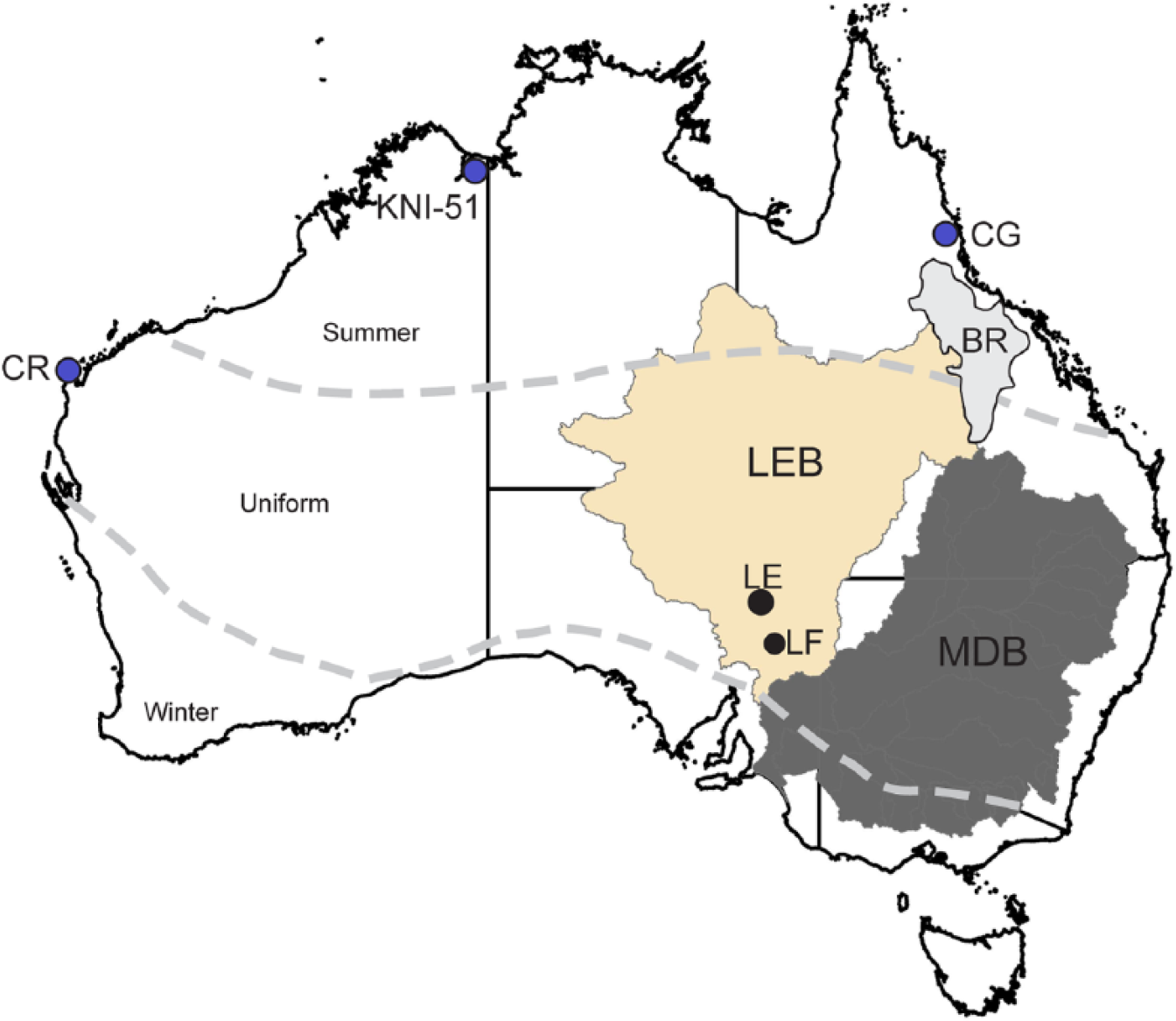
Locality – map of Australia, with the Lake Eyre Basin (LEB) and Kati Thanda-Lake Eyre (KT-LE) and Lake Frome (LF). The Burdekin River (BR) catchment at the headwaters of Cooper Creek is shown, as are stalagmite sites of Denniston et al. (2015; KN1-51) and Haig et al. (2015; CG and CR). MDB is the Murray–Darling Basin.
A number of attempts have been made to document the historical filling of KT-LE with the work of the Lake Eyre Committee (1955) and Bonython and Fraser (1989) providing a useful review to some of the earlier lake-filling events, while Kotwicki (1986) provides a comprehensive assessment of the LEB and the documented timing for filling events in KT-LE based on existing historical compilations. He identifies the years 1891, 1906, 1941, 1949–1951, 1953, 1955–1959, and 1963 as significant filling years on KT-LE. It is unclear, however, as to the magnitude of these previous filling episodes, but the 1974 event is often presented as the largest filling event in historical times, ironically prompting the formation of a yacht club in Australia’s arid interior – the Lake Eyre Yacht Club. This event, which was the wettest year on record for Australia (Ummenhofer et al., 2015), produced lake conditions with maximum depths of ~6.1 m (−9.1 m a.s.l.; Australian Height datum (AHD); Bye et al., 1978; Kotwicki and Isdale, 1991) and maximum lake volumes of 30–32 km3 (Bye et al., 1978; Kotwicki and Isdale, 1991; Leon and Cohen, 2012; Tetzlaff and Bye, 1978). Subsequent work by Kotwicki and Isdale (1991) has attempted to correlate historical KT-LE filling to proxy climate records and large-scale climatic patterns, but with limited geochronological control.
Recent climatic compilations for Australia and the Southern Hemisphere (see Neukom et al., 2014; Reeves et al., 2013) have highlighted the lack of terrestrial records documenting the moisture balance for large areas of the continent and our corresponding limited understanding of past moisture regimes. This is especially the case for the semi-arid and arid zone which comprise ~70% of the Australian landmass. Similarly, we have little knowledge of the range or rate of variability or the timing of climatic extremes. Previous work utilizing shorelines on the adjacent lake basin (the Frome–Callabonna system; Cohen et al., 2012; Figure 1) has shown the presence of extreme wet intervals (1050–1100 CE) during the periods within the Medieval Climatic Anomaly (MCA; 950–1250 CE). But was this a short-lived local phenomenon? More importantly, can we identify continental-wide extremes equivalent to those experienced in 1974 using the much larger KT-LE?
The question of how climatic drivers, such as El Niño-Southern Oscillation (ENSO), have varied throughout the recent geological past is a key area of investigation in the Quaternary sciences. Indeed, the Past Global Changes working group (PAGES) has set out to better quantify the nature of climate change over the last two millennia to put recent multidecadal trends and extremes in the context of long-term change. This has resulted in a concerted effort to better understand climate teleconnections and the spatial variation in climate responses through time across the globe. At a continental-scale climate, reconstructions in Australia have focused on the last two to five centuries (Denniston et al., 2016; Gallant and Gergis, 2011; Gergis and Fowler, 2009), while there have also been increasing attempts to undertake palaeoclimate data-model comparisons over the last 1500 years (see Phipps et al., 2013). However, there is one major impediment to making further progress – a scarcity of terrestrial records for continental Australia that provide unambiguous climate information. This issue has improved somewhat over the last few years with the emergence of a few key records, such as stalagmite records from northern Australia (records of extreme rainfall and flooding events and palaeomonsoon construction; Denniston et al., 2015, 2016), the annual luminescent lines recorded by mid-shelf corals – as an indicator of freshwater runoff into the Great Barrier Reef (Lough, 2007; Lough et al., 2015) – or the tree-ring-derived records and the associated drought index (Cook et al., 2016; Palmer et al., 2015). Such records have yielded the best resolution terrestrial records but in the case of the coral and tree-ring records only for the last four to five centuries.
The recent work by Denniston et al. (2015) suggests, based on stalagmites in the tropical north of the Australian continent (Figure 1), that substantial multi-centennial variability in extreme rainfall occurred between 850 and 1450 CE as a result of enhanced La Niña–like conditions in the tropical Pacific Ocean. In contrast, low numbers of extreme rainfall events were recorded both before and after the MCA (950–1250 CE), during 500−850 CE and 1450–1650 CE a period they interpret to be dominated by enhanced El Niño–like conditions (Denniston et al., 2015). In today’s climate, tropical cyclones deliver large amounts of precipitation to the northern margins of the continent (Villarini and Denniston, 2016) and are primarily responsible for extreme rainfall totals, but these relationships weaken in a southern direction in the headwaters of the LEB. Haig et al. (2015) using stalagmites from northeastern Australia have suggested that one of the greatest periods of cyclone activity over the last 1500 years in the northeast (NE) of the Australian continent occurred in the latter stages of the ‘Little Ice Age’ (LIA, 1300–1870 CE), between 1700 and 1800 CE. However, they also identify two equivalent peaks in cyclone activity in northwest (NW) Australia within the MCA. Thus, the timing of peak pluvials/extreme La Niña conditions, their drivers, the spatial coherence of these events, and the landscape response remains unresolved, especially for the continental interior.
As such, there is a clear need for unambiguous terrestrial palaeoclimate records that clearly and directly depict precipitation/runoff for areas away from the continental margin. We address this issue by examining the shoreline sequences of KT-LE (Australia’s largest lake), with the aim of identifying past extreme pluvials equivalent to Australia’s wettest year on record. As such, we aim to (1) evaluate the potential value of optically stimulated luminescence (OSL) in dating geologically young (including modern) lake shoreline deposits, (2) reconstruct a history of wet extremes using such deposits as past indicators of extreme runoff, and (3) compare these with existing key records on the margins of the continent. When KT-LE fills, it represents a major wet season (as seen in 1974 and 2011) and not only reflects widespread rainfall in the north, northeast, or NW of the continent but also occurs synchronously with above-average rainfall in the entire northern half of the continent (Ummenhofer et al., 2015).
KT-LE
KT-LE, the fourth largest terminal lake in the world drains 1.14 million km2 and has a drainage area that spans over 10° of latitude (Figure 1) and has two lake basins, KT-LE North and KT-LE South, joined via the Goyder channel (Figure 2). Multichannel river systems (the ‘Channel Country’) drain to the lowest point on the Australian continent, passing through low-gradient floodplains (200 mm/km; Jansen et al., 2013) and then through the disrupted drainage network as they negotiate the inland dunefields. Approximately once a decade, floodwaters produced predominantly from tropical moisture in the northern half of the catchment reach the terminal playa of KT-LE (Figure 1). The LEB represents nearly 15% of the entire Australian continent and records a long history of fluvio-lacustrine and aeolian interactions and large-scale biophysical transformations associated with the progressive aridification that has occurred during the late Cenozoic (Tedford and Wells, 1990). Such transformations have shifted the basin from one of megalakes (Cohen et al., 2011, 2015; Magee and Miller, 1998; Magee et al., 2004; Nanson et al., 1998) with active (presumed to be perennial) river systems supporting a diverse ecology of now mostly extinct marsupial, avian, and reptilian megafauna to the dry groundwater-dominated systems seen today. For a detailed review of the modern LEB climatic and physiographic characteristics, we refer readers to Habeck-Fardy and Nanson (2014).
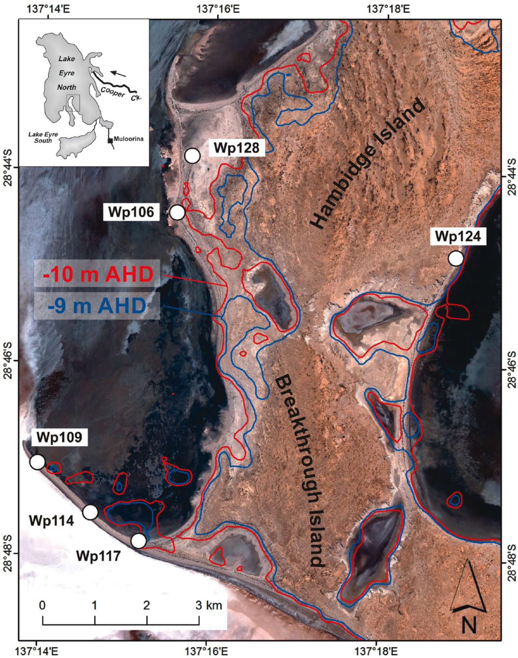
Detailed locality of Hunt Peninsula in Lake Eyre North with the −9 and −10 m AHD contours shown along with the six sample locations (Wpt_109–Wpt_128).
The timing of the late Quaternary megalake phases has been the focus of recent research both in KT-LE (Cohen et al., 2015) and in the adjacent Frome–Callabonna systems (Cohen et al., 2011, 2012; May et al., 2015), but the late Holocene, including the recent millennia, is poorly constrained. KT-LE has only filled to >2 m depth six times in the last four and half decades with 1974 being the largest on record, filling to a maximum depth of ~6 m. Historical aerial photographs from the 1950s demonstrate that many of the major coastal features (e.g. spits) were in existence prior to the largest filling event in 1974. While the 1974 event was important historically and may have deposited beach sediment to the −10 to −9 m AHD water level, it was not solely responsible for the construction of the modern lake shoreline morphology, and as such, shorelines at this elevation are the focus of this pilot study.
Methods
KT-LE is characterized by discontinuous shorelines and spits composed of both sand and gravel (carbonate) clasts and fine-grained near-shore lacustrine silts and muds adjacent to extensive dunefields on the eastern and northern margins of the lake. We targeted one area in the southern end of KT-LE North at Hunt Peninsula where both lake spits and composite shorelines exist between the elevations of −12 and −9 m (Figure 2). Given the remote location and lack of vehicle access, high-resolution differential global positioning system (GPS) was not possible. As such, we employed the use of a Trimble GeoXH static GPS which we then post-processed to the closest permanent base station at Tibooburra, 460 km to the west. This has produced corrected elevations to AHD but with absolute vertical errors ±0.7–0.9 m. We collected point data both for the shoreline sites of stratigraphic investigation and for the 2011 water level, the latter showing excellent consistency between points (n = 8, 13.4 ± 0.2 m AHD; 1 standard deviation (SD)).
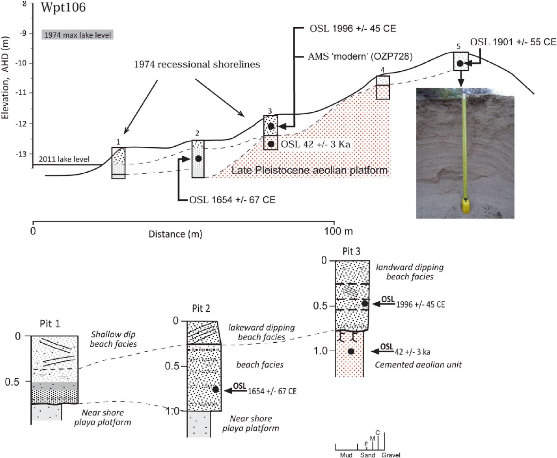
At five locations around Hunt Peninsula, shorelines were excavated to depths of 1.5 m, logged stratigraphically describing facies, grain size, and depositional environment. In total, 11 OSL samples were obtained from between 40 and 150 cm below the surface via hammering stainless steel tubes into the internal face of excavated pits (Figure 2). A modern analog sample was also collected from an active beach as a means of determining the degree of residual OSL signal (Figure 2; Wpt_109) under moderate lake-full conditions. We have employed conventional preparation techniques to isolate the 180–212 µm grain size (Wintle, 1997). The OSL signal of the purified quartz grains was measured using an automated Risø TL/OSL-DA 20 reader equipped with blue light–emitting diodes (LEDs) for stimulation of multigrain aliquots (for initial tests of quartz OSL behavior) and a focused green laser for single-grain measurements (Bøtter-Jensen et al., 2000). The light emitted from both single aliquots and single grains was detected with an EMI 9235QA photomultiplier tube after passing through 6 mm of Hoya U-340 filter to isolate the ultraviolet wavelength. Laser stimulation of individual grains was for 2 s at 125°C, and the first 0.1 s of stimulation with a late background subtraction (i.e. the last 0.3 s of stimulation) was used for OSL signal integration.
We employed the single-aliquot regenerative dose (SAR) protocol and included the following checks of single-grain OSL behavior and SAR protocol performance (Duller, 2003; Jacobs et al., 2006; Murray and Wintle, 2000): Aliquots or single grains were rejected from further analyses if (1) the OSL signal was weak (first test dose signal <3 times the background signal), (2) the sensitivity-corrected zero dose value (recuperation) was >5% of the sensitivity-corrected natural value, (3) the repeat dose points at the end of the measurement procedure were not consistent with the initial value for the same dose (>2σ different from unity), (4) the sensitivity-corrected natural OSL signal did not intercept the dose–response curve, and (5) the OSL-infrared (IR) depletion ratio was more than 2σ below unity, suggesting the presence of feldspar grains or inclusions. For each sample, the external beta and gamma dose rates have been estimated using the values for the concentrations of uranium and thorium determined from thick source alpha counting (via a Daybreak 583 alpha counter) and for potassium by beta counting (using Risø GM25-5 beta counter). An internal alpha dose rate of 0.033 Gy/ka was assumed for the grains based on measurements by Jacobs et al. (2003). For 3 of 11 samples, radionuclide concentrations were determined via inductively coupled plasma optical emission spectrometry (ICP-OES; Table 1). The cosmic-ray dose rates were estimated from equations related to the thickness of the overburden with a correction made for geomagnetic latitude and altitude (Prescott and Hutton, 1994). The present-day moisture content of each sample with a 10% error allowance was used for dose-rate attenuation calculation. All OSL ages within the last millennia are presented as CE calendar years. Where organic material was available (such as fish remains or carbonates from bivalves), we have paired or supplemented the OSL with accelerator mass spectrometry (AMS) 14C measurements (performed on ANSTO’s STAR tandem accelerator; Fink et al., 2004) which are calibrated using CALIB 7.1 with a SHCal13.14c correction (Hogg et al., 2013).
Dose rates and optical ages for Kati Thanda - Lake Eyre sediments.
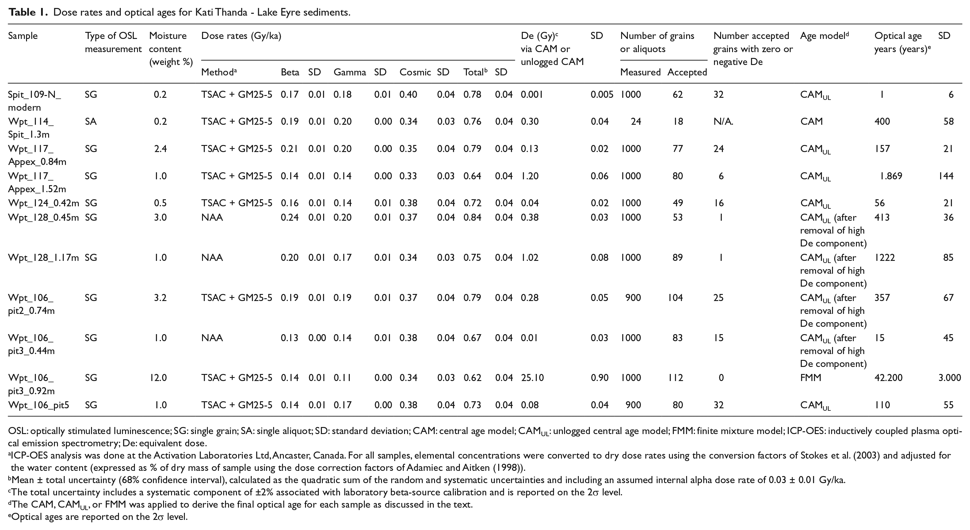
OSL: optically stimulated luminescence; SG: single grain; SA: single aliquot; SD: standard deviation; CAM: central age model; CAMUL: unlogged central age model; FMM: finite mixture model; ICP-OES: inductively coupled plasma optical emission spectrometry; De: equivalent dose.
ICP-OES analysis was done at the Activation Laboratories Ltd, Ancaster, Canada. For all samples, elemental concentrations were converted to dry dose rates using the conversion factors of Stokes et al. (2003) and adjusted for the water content (expressed as % of dry mass of sample using the dose correction factors of Adamiec and Aitken (1998)).
Mean ± total uncertainty (68% confidence interval), calculated as the quadratic sum of the random and systematic uncertainties and including an assumed internal alpha dose rate of 0.03 ± 0.01 Gy/ka.
The total uncertainty includes a systematic component of ±2% associated with laboratory beta-source calibration and is reported on the 2σ level.
The CAM, CAMUL, or FMM was applied to derive the final optical age for each sample as discussed in the text.
Optical ages are reported on the 2σ level.
Results
We conducted dose-recovery experiments on single aliquots (ca. 50 grains per disk) and systematically varied the preheat temperatures for both the regenerative and the test doses in order to determine the most appropriate SAR protocol parameters and to investigate the dependency of recovered equivalent dose (De) on preheat temperature (SOM 1). For this experiment, grains of sample Wpt_106_pit2_0.74m (Figure 2) were sun bleached for 3 days, and a laboratory dose of 30 Gy was administered. The administered dose could be accurately and precisely recovered using a preheat of 160°C for 10 s prior to measurement of the natural and each regenerated OSL signal (Ph1) and 160°C for 5 s prior to measurement of the OSL test dose signals (Ph 2). With this preheat combination, a measured-to-given dose ratio of 1.00 ± 0.06, a recycling ratio of 1.03 ± 0.04, and negligible recuperation (i.e. 0.78 ± 0.34%; weighted average of four aliquots SOM 1) were obtained. Higher preheat combinations resulted in an increase in recuperation and a significant increase in the overall scatter of the data (SOM 1). Using fresh grains from the same sun-bleached sample and identical preheat conditions, the dose-recovery experiment was repeated on the single-grain level, and a measured-to-given dose ratio of 0.99 ± 0.02 was obtained (recycling ratio: 1.02 ± 0.02; 0% overdispersion; n = 37; Figure 3).
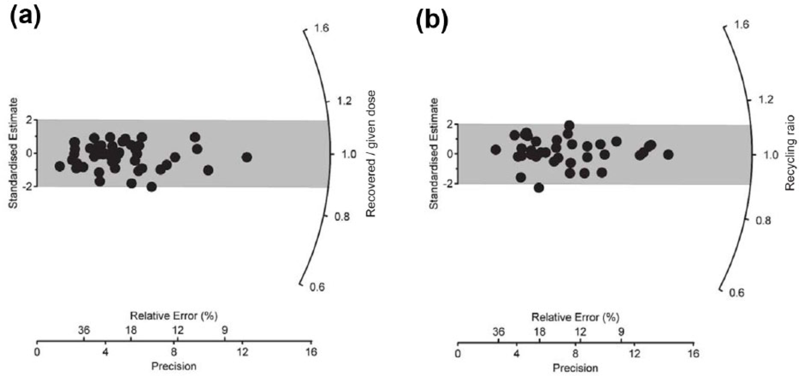
Single-grain dose-recovery experiment for sample Wpt_106_pit2_0.74m (n = 37). The administered laboratory dose was 30 Gy, the preheat 1 was 160°C for 10 s, and preheat 2 was 160° for 5 s. (a) Radial plot showing the recovered-to-given dose ratio (0.99 ± 0.02) and (b) recycling ratio (1.02 ± 0.02).
To further investigate the influence of thermal treatment on De for these very young samples, a thermal transfer test was conducted at the single-grain level. For this purpose, we used fresh sun-bleached grains from sample Wpt_106_pit2_0.74m and repeated the single-grain dose-recovery experiment (Ph 1 of 160°C for 10 s, Ph 2 of 160°C for 5 s), but with a surrogate natural dose of 0 Gy. A dose of 0.05 ± 0.06 Gy (calculated using the unlogged central age model (CAMUL) based on 44 accepted grains out of 500 measured grains; Figure 4) was recovered. In addition, linearly modulated optically stimulated luminescence (LM-OSL) measurements were conducted on two samples, and the results suggest that the KT-LE samples are dominated by the fast component (SOM 2).
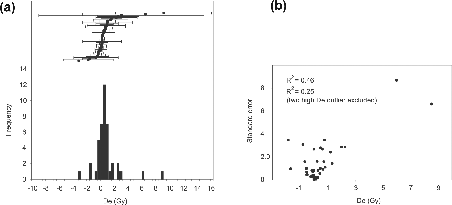
Thermal transfer test for sample Wpt_106_pit2_0.74m on the single-grain level. For this test, the previously established preheat temperature regime (i.e. 160°C/10 s for preheat 1 and 160°/5 s for preheat 2) was used. A dose of 0.05 + 0.06 Gy was recovered (calculated using the CAMUL based on 44 accepted grains out of 500 measured grains). (a) De distribution and standard errors for the recovered single-grain doses plotted as a histogram and (b) De error distribution for the 44 accepted grains; R2 value of 0.25 represents correlation without the two outliers.
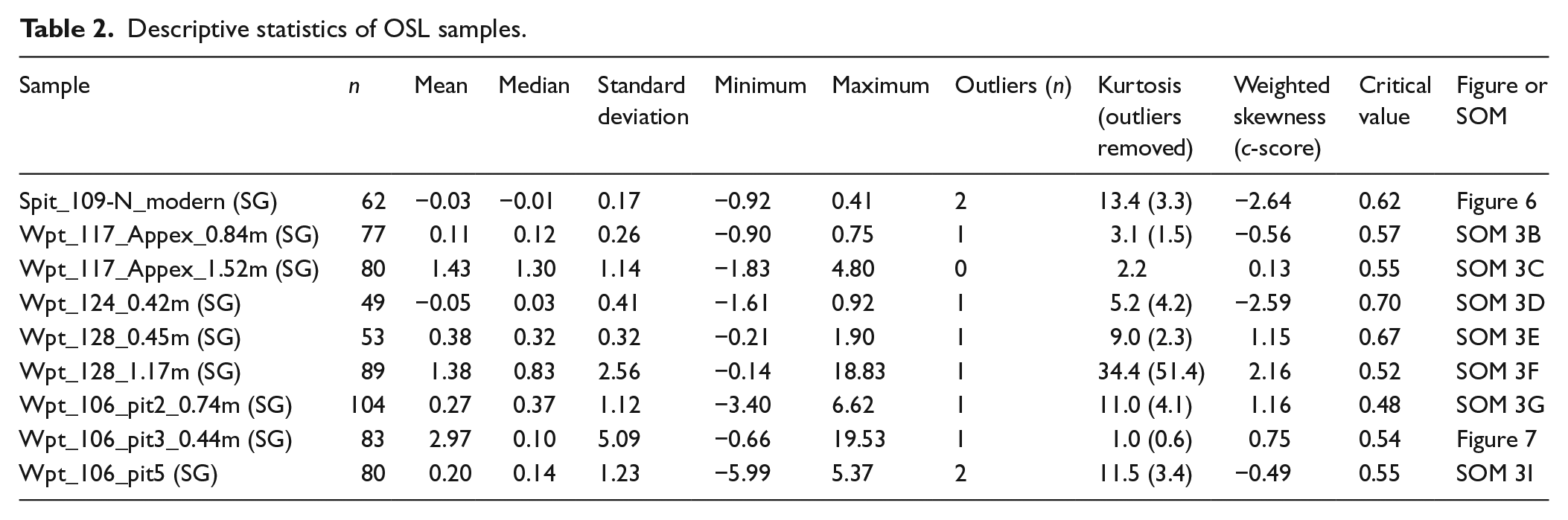
Based on the outcome of these OSL tests, we opted for measuring all samples on the single-grain level using a preheat combination of 160°C for 10 s for Ph 1 and 160°C for 5 s for Ph 2 (with one exception, i.e. sample Wpt_114_Spit_1.3m, which was measured on the multigrain level; Table 1). Typical OSL decay curves and SAR dose–response curves are shown in Figure 5. Construction of dose–response curves involved regenerative dosing up to 8 Gy and 80 Gy for the youngest and oldest samples encountered in this study, respectively. For sensitivity correction during the SAR procedure, test doses between 2 and 5 Gy were used and the SAR growth curves were fitted using either a linear or a saturating exponential function. Zero or negative De values were common in our single-grain data (Table 1) because of the very young or modern age for several of our samples. In order to deal with genuinely zero-age samples or zero-age grain populations (revealing negative, zero, and near-zero De values), we applied unlogged age models for De calculation as discussed below (see also Table 1). For visualization and interpretation of single-grain De distributions that include negative and zero De estimates, we opted for a combined graphical display involving scatter plots and histograms of De estimates and their standard errors. Radial plots are used for samples with De distributions entirely composed of positive single-grain De values. This two-pronged approach in visualizing our single-grain De data was adopted because currently available programs to generate radial plots are not capable of correctly plotting De distributions with a significant number of zero and negative De grains with low precision (as is the case for several samples in this study). The single-grain De distributions for selected samples are shown in Figures 6 and 7 (see SOM 3 for the De distributions of all remaining samples). For all single-grain De distributions that are plotted as histograms (i.e. that involve zero and negative De values), descriptive statistics are provided in Table 2, including the Grubb’s test for outliers, kurtosis (i.e. a measure of the ‘peakedness’ of a distribution with a value of 3 indicative for a normal distribution), and the weighted skewness test (i.e. if the c-score in Table 2 is greater than the critical value, a distribution can be regarded as significantly positively skewed; Bailey and Arnold, 2006). The final optical ages for all samples are given in Table 1.
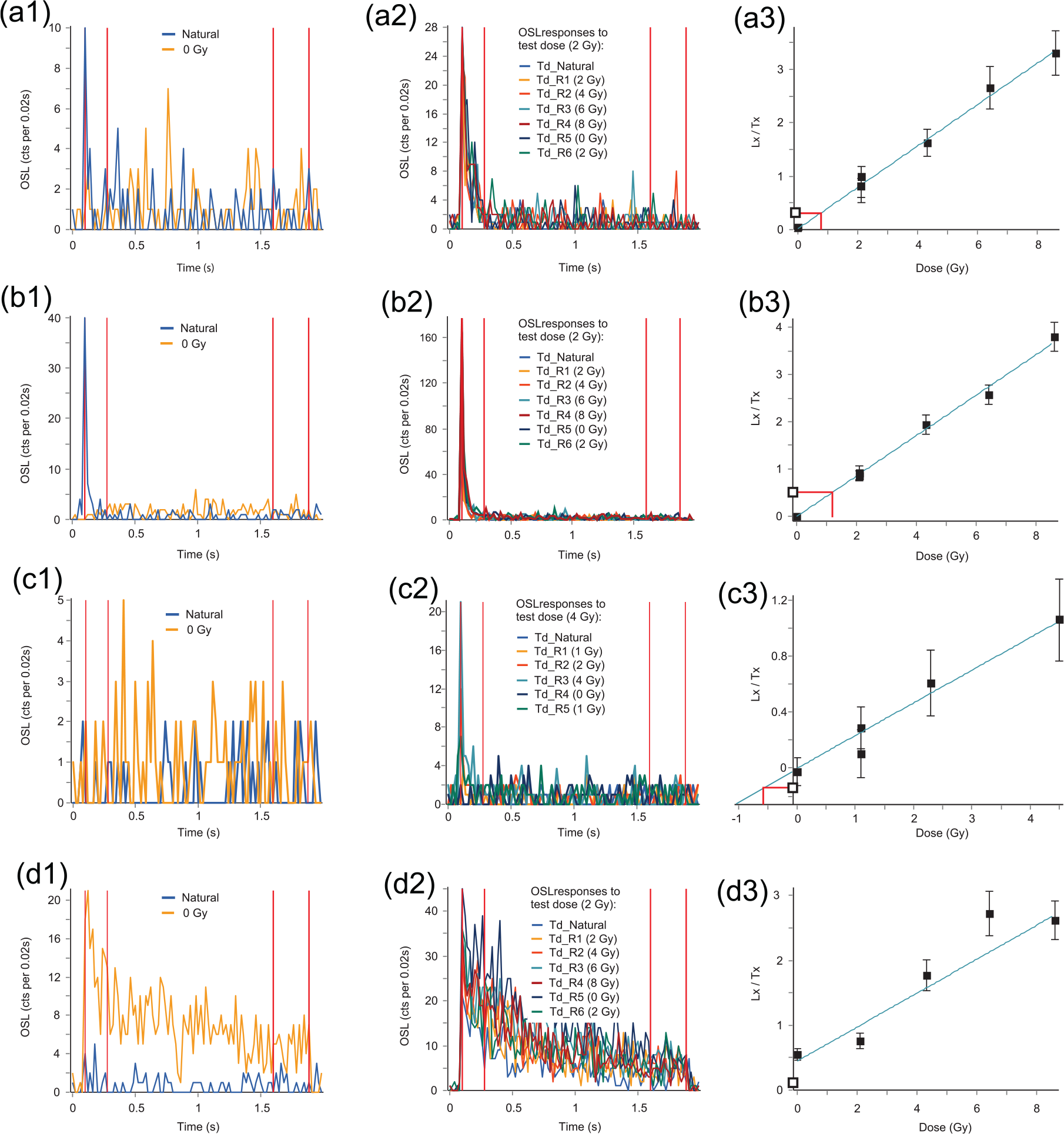
OSL characteristics of four representative single grains of quartz. In the first column (a1–d1) the OSL curves for the natural dose (Ln) and 0 Gy doses are shown. The second column (a2–d2) depicts the OSL responses to the SAR test doses. Third column (a3–d3) shows the SAR dose–response curve. Grain in row a reveals a very weak but measurable natural dose (0.8 ± 0.4 Gy, that is, 50% relative error); grain in row b has a moderate Ln OSL signal and relatively bright regenerated OSL signals, thus allowing the De value to be determined more precisely (1 ± 0.2 Gy, i.e. 20% relative error). Row c shows a modern grain with no natural signal. The signal integration interval is thus dominated by dark counts. The dark counts in the background integration interval of the natural OSL curve happen to be slightly higher than the dark counts in the signal integration interval (c1), thus causing the De value for this grain after background correction to become negative (c3). A grain with an aberrant OSL behavior is shown in row d (abnormal slow OSL decay), resulting in significant recuperation (details see text).
(a) Single-grain De distribution for sample Spit_109-N_modern (n = 62) plotted as histogram. (b) De error distribution for 62 accepted grains.
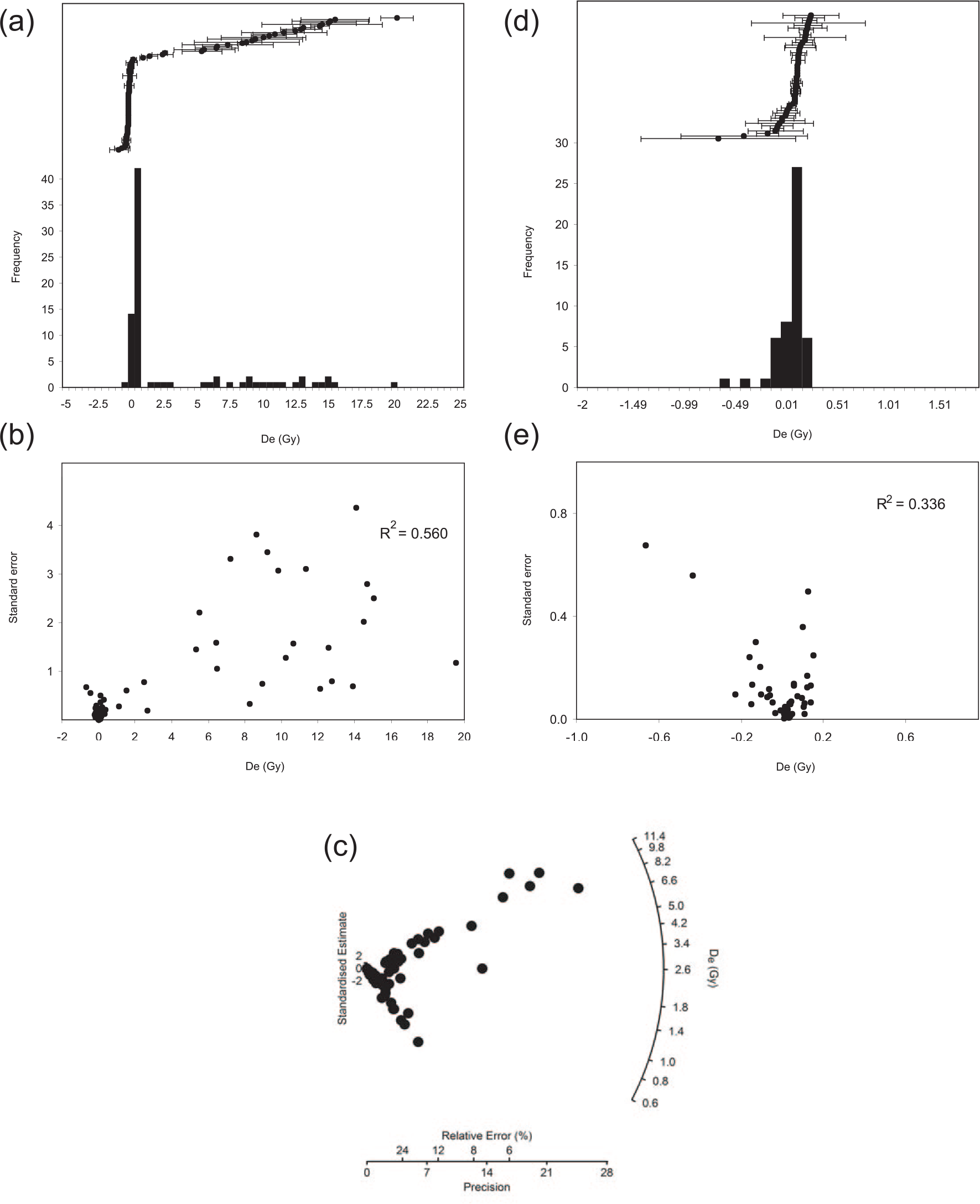
(a) Single-grain De and error distributions for sample Wpt_106_pit3_0.44m (n = 83). (b) Single-grain De estimates plotted as a histogram with corresponding De error distribution. (c) Radial plot of single-grain De estimates (for this plot, all grains with negative or zero De values were set to 0.001 Gy, while the standard errors remained unchanged). The radial plot confirms the existence of a distinct low and a high De component in this sample. (d and e) Single-grain De and error distribution, after the high De component has been removed from the data set.
Descriptive statistics of OSL samples.
Chronostratigraphy of the KT-LE shorelines
All surface elevations of our shorelines range from −11.8 m (the lowest on Hunt Peninsula; Figure 2) to −8.5 m (Figure 2), and peak lake levels in 1974 were −9.1 m AHD (±0.45 wave height uncertainty as recorded by Dulhunty, 1975), indicating that all shorelines examined in this study were at or below the peak 1974 water level. The multiple and composite shorelines that exist between −11.8 and −8.5 m AHD suggest that the modern maximum lake levels are all capable of inundating and potentially building and modifying these sedimentary features. Water level at the time of our sampling was below these shoreline elevations (−13.4 ± 0.2 m), and the filling extent/depth in 2010/2011 was comparable (albeit a little smaller) to 1989 and 1997 but smaller than 1984 and half the depth of 1974. The geochronology and stratigraphy of the shorelines have important implications on the likely frequency of extreme wet phases such as 1974 and are discussed below.
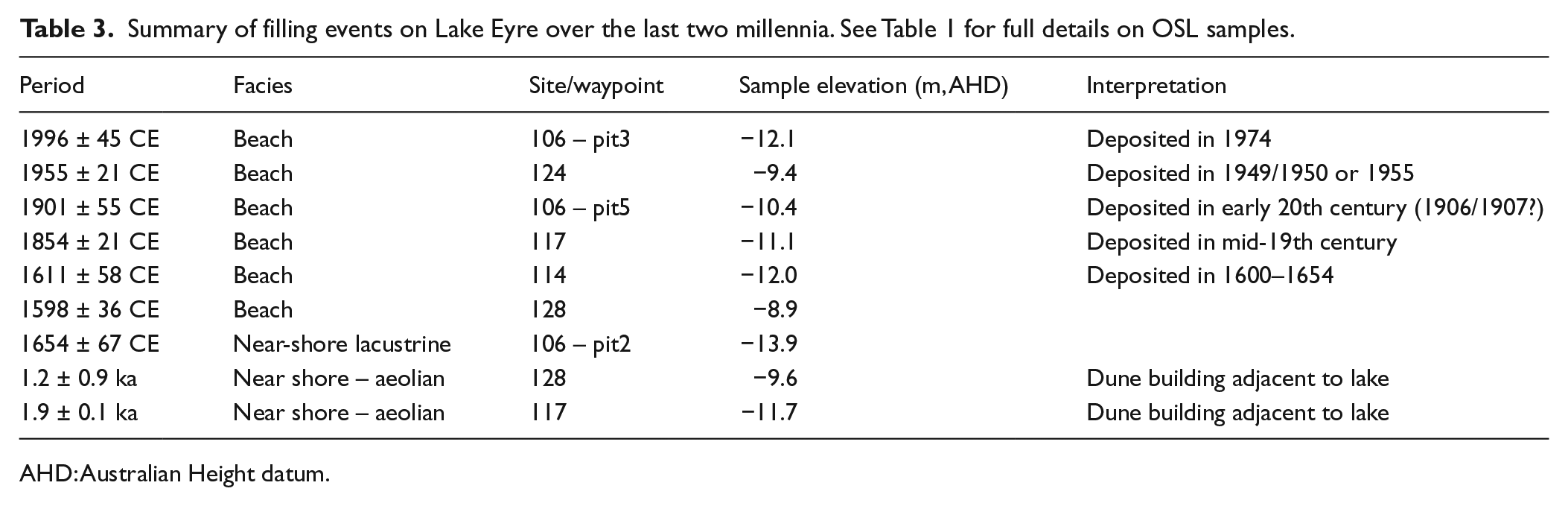
Table 3 presents a summary of sample elevation, depositional environment and the respective ages. Our analysis of 13 samples highlights the spectrum of deposits encountered on the margin of the modern KT-LE ranging from beach to near-shore lacustrine facies and near-shore aeolian facies. Composite shorelines exist and are characterized by poorly sorted coarse sand and pebbly beach facies with landward dipping foresets (Figure 8). In some cases, we can constrain that the deposits themselves are lenticular and drape preexisting (late Pleistocene) near-shore aeolian deposits, separated by an erosional unconformity. At our primary transect, where we have five excavations, three major depositional beach units overlie basal indurated aeolian sands (Figure 8). The uppermost of these beach facies is dated to 1996 ± 45 CE (which we interpret to be deposited in 1974) and contains fish vertebrae and plant remains (yielding modern AMS ages – Table 4 and Figure 8). This beach facies extends over multiple excavations at this transect and is expressed topographically as a series of low-relief shorelines that presumably reflect recessional deposits from the 1974 event. Sitting at a slightly higher elevation is the oldest of the 20th-century deposits, with one sample yielding an age of 1901 ± 55 CE. This beach facies (also landward dipping) is interpreted to represent lake filling in the early 20th century (possibly 1906 or 1908 as identified by Kotwicki, 1986). On the eastern side of Hunt Peninsula, we successfully capture a mid-20th-century filling event with one sample from a coarse-grained deposit yielding an age of 1955 ± 21 CE. All of the 20th-century samples stem from elevations that range from −13.9 to −8.9 m AHD (all within the range of modern historical filling events).
Summary of filling events on Lake Eyre over the last two millennia. See Table 1 for full details on OSL samples.
AHD: Australian Height datum.
AMS 14C results with calibration using CALIB 7.1 and SHCal13.14c (Stuiver et al., 2017).
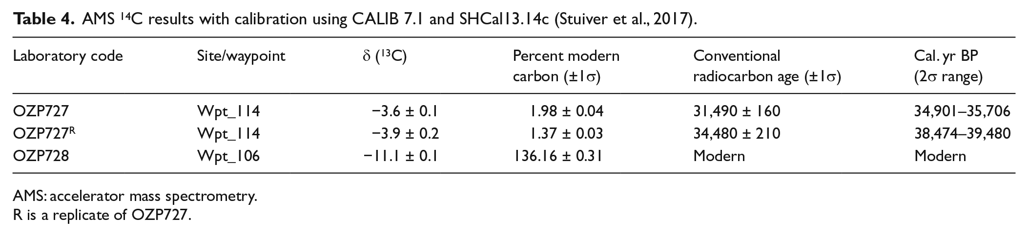
AMS: accelerator mass spectrometry.
R is a replicate of OZP727.
We also record two other filling intervals in the 19th and 17th centuries with one site recording beach facies deposition in 1854 ± 21 CE and three other sites recording beach or near-shore lacustrine sedimentation between 1598 ± 36 CE and 1654 ± 67 CE (Table 3). Given the varying elevations of these three samples (5 m vertical spread), we assume that peak lake level was −8.9 m (±wave height uncertainty) for this early 17th-century lake-filling event. Two other sites record depositional evidence that is ambiguous and could either represent well-sorted near-shore beach facies or source-bordering aeolian deposition. The OSL ages for these sites are 1.2 ± 0.09 ka (Wpt_128; Figure 2) and 1.9 ± 0.14 ka (Wpt_117; Figure 2 and Table 1).
Discussion
Inherent to optical dating of young and modern sediments are a number of methodological challenges that have to be adequately addressed before an interpretation of OSL chronologies from samples of the recent geological past can be reasonably attempted. These challenges include (1) low luminescence sensitivity, that is, young and modern samples frequently reveal dim OSL signals because of the low doses absorbed during the short periods of burial time. As a result, natural OSL signals from modern samples are often barely discernible from background noise, impairing the precision with which De estimates can be determined. This is particularly true when measuring individual grains of quartz because of the lower luminescence sensitivity on the single-grain level compared with the multigrain level (e.g. Ballarini et al., 2007a, 2007b; Jain et al., 2004; Medialdea et al., 2014; Thomsen et al., 2003); (2) thermal transfer that might occur during preheating can transfer charge from light-insensitive traps to light-sensitive ones (Rhodes, 2000; Wintle and Murray, 2000). Such transfer will cause problems if it is a significant fraction of the natural signal, leading to overestimates in palaeodose and hence optical ages (e.g. Bailey et al., 2001; Kiyak and Canel, 2006); (3) alterations in the sedimentary environment (e.g. changes in water content or sample depth and degree of compaction over time) can cause dose rates to become time-dependent. Especially in rapidly accreting sedimentary environments, some of these changes can be more pronounced at the beginning of the burial history rather than be linear in time (e.g. compaction and dewatering; variations in gamma and cosmic dose rates), therefore affecting the dosimetry of young and modern samples more intensively compared with geologically old samples (e.g. Madsen et al., 2005); (4) identification of incomplete bleaching is critical in young sediments because the dose retained by incompletely reset grains might be considerable compared with the burial dose (e.g. Ballarini et al., 2007a; Jain et al., 2004; Medialdea et al., 2014). Moreover, (v) any type of sediment mixing that causes intrusion of grains with a higher (or lower) burial dose into young strata will have – if unrecognized – a particularly adverse effect on the optical age estimate of young sediments (e.g. Reimann et al., 2012; Rink et al., 2013).
In the following, each of these methodological aspects that adhere to OSL dating of young and modern sediments is discussed for the investigated shoreline samples from KT-LE, and the implications in the context of this dating study are considered.
Luminescence sensitivity and single-grain De distributions containing negative De values
For single grains of quartz that were extracted from young or modern samples and that passed the rejection criteria, we observe low signal-to-noise ratios for the natural OSL signal, but good OSL responses to the test doses as well as increasing OSL responses to the successive regenerated doses (Figure 5a and b). Grains lacking a natural dose luminescence signal (Ln), but otherwise satisfying the OSL quality criteria, were assumed to be modern in age and also accepted. For several of the grains with very low or no Ln signal, however, the signal-to-noise ratio was
For each KT-LE sample, 6–12% of the measured grains passed all rejection criteria, suggesting that despite the low signal-to-noise ratio of the Ln signal, the intrinsic grain brightness of these samples (as measured by the test dose OSL signal) is comparable with single-grain OSL studies where much older sediments were dated (e.g. Jacobs et al., 2011: 5–30% for late Pleistocene cave mouth sediments from Morocco; Cohen et al., 2011: 3–17% for late Pleistocene shoreline sediments from central Australia). Most single-grain OSL studies on young sediments report a much lower intrinsic grain brightness (e.g. accepted grains in Ballarini et al., 2007a: 4–5%; Jain et al., 2004: 0.3%; Medialdea et al., 2014: 2%; Thomsen et al., 2003: 0.3–1.5%). Although we observe relatively high intrinsic grain brightness in our samples, the signal-to-noise ratio for the Ln OSL signal in the very young and modern KT-LE samples is still low. This can be attributed to the (inevitable) dominance of random noise over very low natural signal intensities and results in poor precision (i.e. a high relative standard error (RSE)) for the youngest of our single-grain De estimates. For those samples from KT-LE that are a few decades to a few centuries in age, the RSE in single-grain palaeodose estimates ranges from 9% to 50% (20% on average; Table 1). Very similar precisions on De estimates have been obtained in other single-grain studies on young sediments published so far (e.g. Jain et al., 2004: RSE of 13–32% for 40-year-old mortar samples; Ballarini et al., 2007a: RSE of 7% and 14%, respectively, for two subsamples from a ca. 300-year-old coastal dune ridge; Medialdea et al., 2014: RSE of 25–30% for samples a few decades in age and 6–10% for samples that are between 1 and 10 centuries old – all from slack-water deposits). Only the modern analog sample (Spit_109-N_modern) has a De estimate with a RSE of 500%, resulting in an optical age of 1 ± 6 years (Table 1). Yet, while the precision is low for this sample, it is – within dating errors – still a genuinely modern sample and the optical age thus accurate.
Thermal transfer and OSL signal composition
With the low preheats used in this study, we did not expect any significant thermal transfer of charge to occur, an expectation confirmed by the results of our thermal transfer experiment (Bailey et al., 2001; Kiyak and Canel, 2006; Rhodes, 2000; Wintle and Murray, 2006; Figure 4). However, very low preheats might fail to remove thermally unstable components that can result from laboratory irradiation, which, in turn, might adversely affect the accuracy and precision of the resulting SAR De estimates (Choi et al., 2003; Jain et al., 2008; Thomas et al., 2005; Tsukamoto et al., 2003). In this study, the thermal transfer experiment and the SAR dating runs were conducted on the single-grain level, and all accepted grains revealed OSL decay curves that reached background during or shortly after the first 0.1 s of stimulation (Figure 5a–c), suggesting that the OSL signal of these grains is dominated by the fast component. This finding is corroborated by the LM-OSL measurements conducted on the multigrain level for the same samples (SOM 2). However, some grains are characterized by OSL decay curves of the test dose signals and the regenerated dose signals that did not reach background even after 2 s of green laser stimulation (Figure 5d), resulting in recuperation values well above 5% (
Alterations in the sedimentary environment and dose-rate calculation
All the OSL samples are from well-drained medium to coarse-grained sandy deposits with burial depths between 40 and 150 cm, where post-depositional compaction and changes in the sedimentary texture and thus changes in the water content (if any) were minor. Because of the arid environment at KT-LE (200 mm/yr precipitation), infiltration from above or below (e.g. groundwater fluctuations that might alter soil moisture or radionuclide concentrations) is also negligible. Furthermore, hydrological evidence suggests that the historical shorelines most likely accreted rapidly as peak lake level is only maintained for
OSL signal resetting in KT-LE shorelines
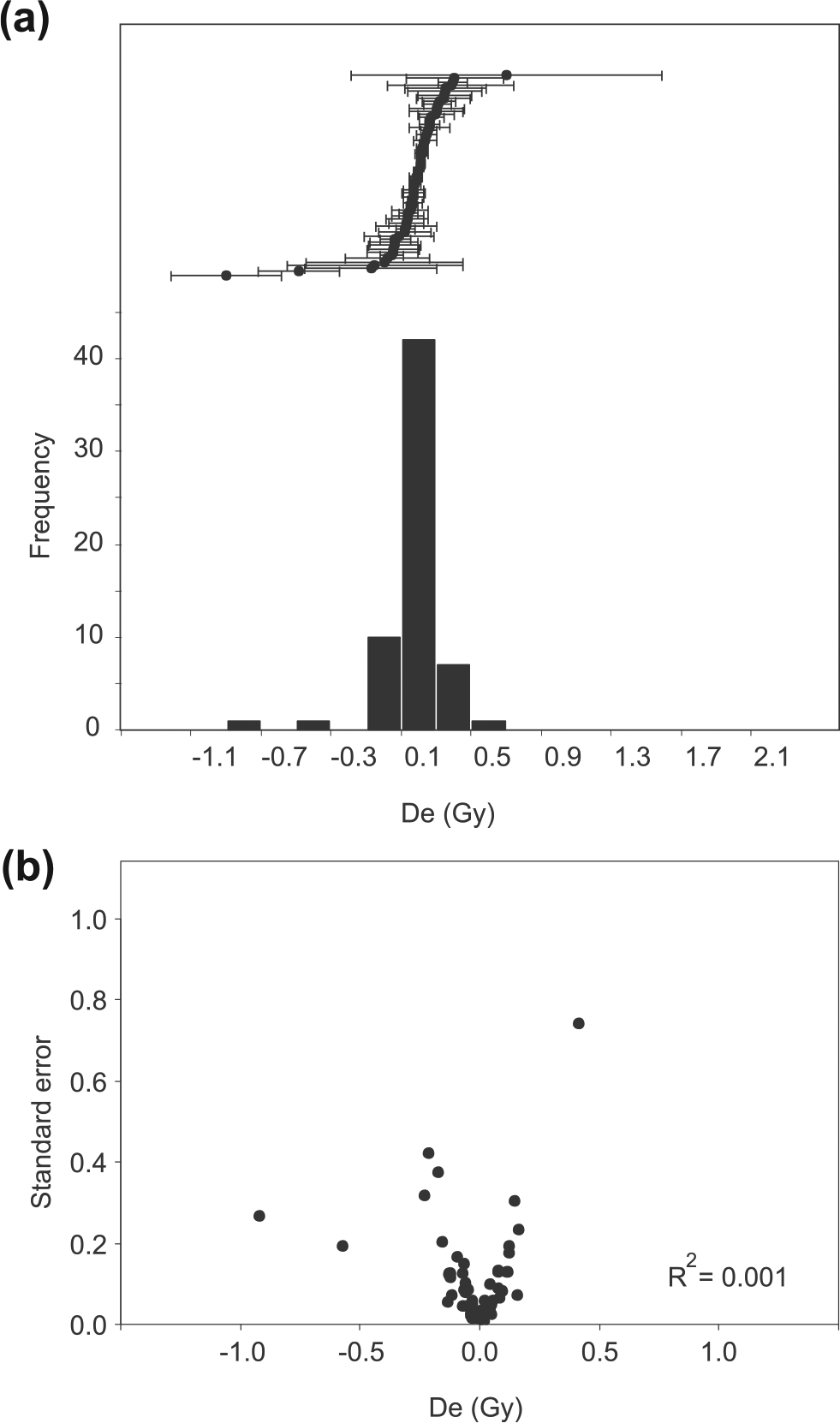
One sample was obtained from a modern shoreline that formed during the high stand in 2009–2011 (i.e. Spit_109-N_modern; validated via analysis of satellite imagery and during our field survey). The single-grain De distribution for this sample is shown in Figure 6. Visual inspection suggests that the De distribution is centered on a very low De value close to 0, has a kurtosis of 13.4, and also contains two negative De outliers (Table 2). The weighted skewness test is negative (i.e. no indication for a positively skewed single-grain De distribution that would suggest partial bleaching). Removing the two negative De outliers from the De distribution results in a kurtosis of 3.3 (i.e. an almost ideal normal distribution) and a weighted skewness test that is still negative. It is, therefore, concluded that this modern analog sample from a beach facies has been adequately bleached prior to deposition. Using the CAMUL (Arnold et al., 2009), we obtain an optical age of 1 ± 6 years, suggesting that a very low (essentially modern) De value can be accurately measured with the optimized SAR protocol parameters. In total, four more single-grain De distributions that contain near-zero, zero, and negative De values pass the weighted skewness test and also broadly resemble normal distributions (i.e. samples Wpt_117_Appex_0.84m, Wpt_117_Appex_1.52m, Wpt_124_0.42m, and Wpt_106_pit5; Table 2 and SOM 3). For these samples too, complete resetting of the OSL signal prior deposition arguably occurred, and the CAMUL has been applied to each of these single-grain De distribution for palaeodose calculation (Table 1).
Sediment mixing
For the samples Wpt_128_0.45m, Wpt_128_1.17m, Wpt_106_pit2_0.74m, and Wpt_106_pit3_0.44m, the single-grain De distributions are asymmetric and broad, and the weighted skewness tests suggest a significant positive skew in each of these distribution. The single-grain De distribution of sample Wpt_106_pit3_0.44m serves as a good example for this type of skewed De distribution and is depicted in Figure 7. The De values of this sample are clearly clustered on a very low De value, but a significant number of grains also carry palaeodoses that are higher by one to two orders of magnitude (Figure 7a). To better evaluate the shape of this particular single-grain De distribution, which includes grains with a wide range in precision (Figure 7b), all zero and negative De estimates were set to 0.001 Gy (the standard error remained unchanged) and the modified De distribution was visualized via a radial plot. From the radial plot, it becomes obvious that two distinct De populations are present in this sample, with a low De component congruent with a palaeodose in the order of several tens of milligray (60% of the grains), and a high De component centered on ca. 11 Gy (Figure 7c). We do not observe a continuous (or semi-continuous) spread of single-grain De values from high to low De values, as would be expected for a partially bleached sample (e.g. Duller, 2004). The same basic observation applies to the three other aforementioned positively skewed single-grain De distributions (see SOM 3). It is also interesting to note that in each of the samples that reveal an asymmetric single-grain De distribution, the low De population comprises the vast majority of grains (i.e. 60–97%; Table 2). We reject partial bleaching as the main cause for the positive skew in these De distributions because (1) two distinct De populations rather than a continuous spread of De values are observed in all of these distributions, and (2) no evidence for incomplete resetting was found in the modern analog sample or any other of the young shoreline samples investigated so far.
A plausible explanation for the presence of high De grains or distinct high De components in a De distribution that is dominated by low or very low De grains is pedoturbation by burrowing animals. This type of sediment mixing can affect the uppermost 1–2 m of the sedimentary substrate and often results in a preferential upward movement of grains from deeper into younger strata and even exhumation of grains to the surface (Bateman et al., 2003, 2007a, 2007b; Rink et al., 2013). Ongoing research suggests that upward translocation of sand grains by animals is mainly related to nest excavation (e.g. burrowing of ants; Rink et al., 2013) or small mammals (e.g. gophers; Bateman et al., 2003). These studies also suggest that a relatively small flux of downward movement of grains occurs (mainly due to back-filling by nest collapse). For our samples that reveal a skewed De distribution, (1) we propose that it is the low De component (comprising 60–97% of the grains; Table 5) that is representative of the true depositional event, and (2) we assume that burrowing animals that moved deeply buried grains upward into shallower levels are responsible for the presence of high De grains in our single-grain De distributions. This suggestion is supported by our observations made during the field campaign in 2011 (i.e. at the end of an unusual long wet period), when small mammals were particularly common and fresh traces of their burrowing activity ubiquitous (SOM 4).
Results of the finite mixture modeling.
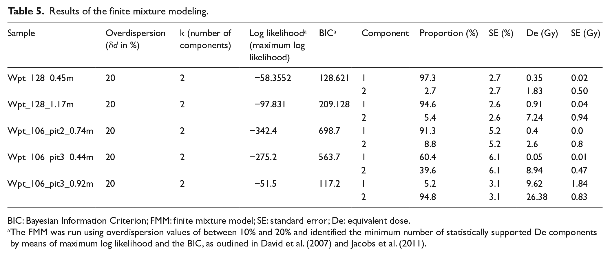
BIC: Bayesian Information Criterion; FMM: finite mixture model; SE: standard error; De: equivalent dose.
The FMM was run using overdispersion values of between 10% and 20% and identified the minimum number of statistically supported De components by means of maximum log likelihood and the BIC, as outlined in David et al. (2007) and Jacobs et al. (2011).
To ultimately derive a palaeodose from such mixed samples, we applied the following strategy: (1) identification of intrusive high De grains on statistical grounds (high kurtosis and weighted skewness values) and via inspection of single-grain De distributions (combining histograms and radial plots); (2) isolation of the high De component through the application of finite mixture modeling (all zero and negative De values were first set to 0.001 Gy; Table 5) and removal of this high De component from the single-grain De data set; and (3) application of the CAMUL to the remaining low De grains (all 0.001 Gy grains were set back to their original zero or negative De values). We note that the adjusted single-grain De distributions (i.e. those for which the high De component has been removed) did all pass the weighted skewness test and revealed kurtosis values in broad agreement with a normal distribution.
Identifying extreme pluvials in continental Australia – A proxy comparison
The resulting chronology obtained from the shorelines represents the first numerical dating of ‘recent’ filling events in KT-LE. Major flooding episodes in the LEB are most often associated with La Niña phases of ENSO, and during such times much of the continent experiences enhanced austral summer monsoon activity (including tropical cyclones; Villarini and Denniston, 2016) and incursions of the monsoonal system in central Australia (Allan, 1985). In today’s climate, lag correlations exist in the east of the LEB (i.e. in the headwaters of Cooper Creek) between spring rain and winter Southern Oscillation Index (SOI) and also between summer rain and spring SOI (McMahon et al., 2008). The strength of these ENSO-rainfall teleconnections varies on interdecadal timescales, and indeed, interdecadal variability is a strong feature of the eastern Australian climate. This has been investigated with regard to Pacific sea surface temperature variability, termed the Interdecadal Pacific Oscillation (IPO) or the Pacific Decadal Oscillation (PDO; Power et al., 1999). A positive IPO phase is associated with warming across the tropical Pacific and cooling of the north and south Pacific; the opposite occurs during the negative phase. Figure 9 shows the SOI over the last 130 years, the IPO phases for the same period along, predicted tributary inflows to KT-LE (Kotwicki and Isdale, 1991), and reconstructed annual discharge on the Burdekin River (Lough et al., 2015). The latter river is east flowing (compare Figure 1), and these proxy data together with the inflow model of Kotwicki (1991) currently provide the best empirical data set for historical filling events of KT-LE over the last century (river gauge data only exist since the early 1970s). What is clearly apparent from Figure 9 is that major predicted lake inflows to KT-LE occur when the SOI is positive (strong la Niña) but also when the IPO is negative (e.g. 1890, 1920, 1950, 1974, and 2011). This agrees well with the recent four decades where the two largest la Niña events produced exceptional stream discharge and lake filling (blue bars of 1974 and 2011 in Figure 9). In most instances, these filling events also coincide with high values of predicted annual discharge on the Burdekin River, showing the correlation between these two systems which share a catchment divide (Kotwicki and Isdale, 1991).
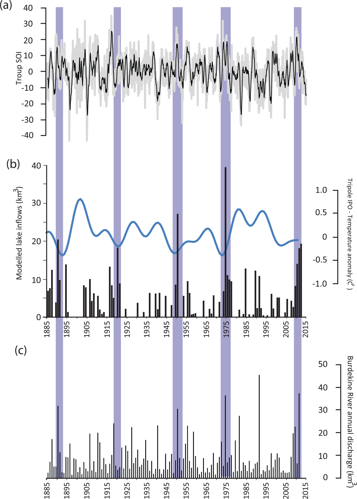
(a) Troup monthly Southern Oscillation Index (SOI) – gray line with 7-point moving average (black line) – Australian Bureau of Meteorology; (b) modeled Kati Thanda-Lake Eyre inflows (black bars) from Kotwicki (1991) and Kotwicki (unpublished data) and Interdecadal Pacific Oscillation tripole index (TPI – blue line; based on filtered ERSSTv3b monthly data; Henley et al., 2015); and (c) reconstructed Burdekin River annual discharge from Lough et al. (2015). Major KT-LE filling shown with vertical blue shading based on historical records.
Our shoreline ages generally support this (Figure 10); however, our error estimates of 2–4 decades on individual ages prevent us from precisely prescribing certain lake-full events to known historical filling intervals. For example, our estimated age of 1901 ± 55 years at our main transect (Wpt_106; Figure 8) is within errors of another site dated to 1955 ± 55 years (Wpt_104; Figure 2). Both shorelines have similar elevations (Table 3), and it is plausible that both formed in the largest lake-filling event in the first half of the 20th century in 1949/1950 (Kotwicki and Isdale, 1991). In the modern hydrological regime, previous work has shown that the tropical influences during the austral summer and autumn dominate significant daily precipitation occurrences in the KT-LE catchment (Pook et al., 2014). Indeed, over 70% of the heavy daily rain events in the LEB occurred when the SOI was in its positive phase (La Niña phase). These heavy rainfall days are characterized by convergence in a monsoon trough over northern Australia or, at the very least, a well-defined trough of low pressure in easterly airflow. Thus, it is not unreasonable to assume that peak lake-filling events, as documented for the mid to late 19th century and earlier, were also driven by extreme La Niña conditions as seen in 1974 and 2011.
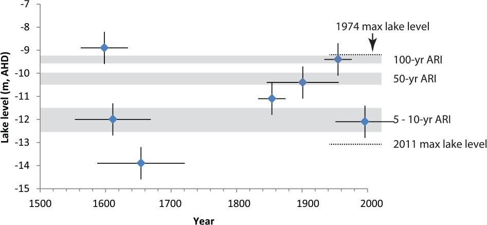
Age-elevation diagram of Lake Eyre based on OSL ages and average recurrence intervals (ARI) of filling levels based on Kotwicki and Isdale (1991). All ages are from horizontally bedded or landward dipping poorly to moderately sorted beach facies.
The 1854 ± 21 CE shoreline sample is within error of the second largest predicted annual flow on the Burdekin River in 1870 (Lough et al., 2015), suggesting major runoff to KT-LE via Cooper Creek which shares headwaters and hydrological characteristics with the Burdekin River (Figure 1; Kotwicki and Isdale, 1999). The other three sites record beach or near-shore lacustrine sedimentation between 1598 ± 36 CE and 1654 ± 67 CE. However, given that the three OSL ages of these shorelines overlap within errors and stem from three different locations, and different elevations, we cannot readily resolve whether these represent three individual filling episodes or were deposited during one lake-filling event. The existing terrestrial/coastal records for northern and northeastern Australia in which to compare these (single or multiple) pluvial event(s) include the following: (1) recent drought indices (based on regional average summer Palmer Drought Severity Index) suggesting a peak pluvial, equivalent to 1974 or 2011, having occurred in 1572–1573 (Cook et al., 2016); (2) a cyclone activity index (Haig et al., 2015) indicating elevated cyclone activity, relative to present over northwestern and northeastern Australia, from 1650 to 1690 (see Figure 1 for cyclone sites). We note that our shoreline ages fall between these two intervals. Finally, (3) a sea-salt record from Law Dome, Antarctica, that has been used as a far-field proxy for eastern Australian rainfall amount and for the reconstruction of the IPO (Vance et al., 2013) is available for comparison too. While KT-LE is not in eastern Australia, annual rainfall in the headwaters of Cooper Creek (one of two major tributaries to KT-LE) has a strong correlation to the sea-salt record at Law Dome (Vance et al., 2015). Indeed, this reconstruction of the IPO identifies a major IPO negative phase in 1609 CE falling midway between the documented shoreline ages and corresponds with previous estimations by Gergis and Fowler (2009) for extreme La Niña events from the 1520s through to the 1660s. However, this is not recorded as a peak pluvial in the recent Cook et al. (2016) drought atlas, highlighting the need for robust terrestrial records that actually record such wet extremes.
Conclusion, lessons, and outlook
The shorelines of KT-LE were investigated over four decades ago by Dulhunty (1975), but in the absence of absolute age control, these shorelines were assigned arbitrary dates of formation of between 500 and 3000 years before present. In contrast, our proof of concept study has shown the value of applying the advanced capability of single-grain OSL dating to discontinuous archives from ephemeral landforms such as lake shorelines, which by their nature record the peak runoff in a given extreme pluvial season(s). We show that many shorelines around Australia’s largest lake are composite features and thus potentially record multiple peak pluvials. However, a more systematic collection of samples from a broader range of lake-margin locations, including more substantive excavations at sites that yielded ambiguous lake-filling evidence, remains to be conducted. It is only with a larger data set that drivers of hydroclimate variability over the last millennia and the delivery of moisture to the arid interior can effectively be evaluated. What can be readily ascertained, however, is that the shorelines around KT-LE record a history of extreme pluvials akin to 1974 and 2011.
We have shown the value of OSL, in particular single-grain OSL, in dating lake shorelines constructed as recently as the mid to late 20th century. Modern shorelines (formed in 2011) yield well-bleached samples with no residual signal and a zero age. Despite a relatively low signal-to-noise ratio, given the youthful nature of the deposits and the low dose rates, the distribution of De values identifies the well bleached, but in some cases, bioturbated nature of these deposits. From this, we have successfully captured the deposition of lake shoreline facies that occurred in peak pluvials, including historical filling events such as 1974 and 1949/50. These wet phases in the historical data set correspond to enhanced La Niña years and IPO negative phases. Two major continental-scale pluvials are identified in 1854 ± 21 CE and 1598–1654 CE with the former corresponding well to other proxy data from northeastern Australia suggesting pronounced runoff via Cooper Creek. Two additional periods of potential lake filling have been identified at 1.2 ± 0.09 and 1.9 ± 0.14 ka, but these require further validation. We believe that assessing the spatial coherence of Australian lake shore records and thus constraining the regional signature of particular La Niña periods, over the last millennia and beyond, provide immense scope for future research.
Footnotes
Acknowledgements
The authors would like to thank the Arabuna community for allowing access to Hunt Peninsula and the South Australian Department of Environment, Water and Natural Resources for the research permit.
Funding
This work was undertaken through funding made available to TC via the Australian Research Council Discovery Program (DP1096911).