Regional hydrologic synchrony in the Southeastern United States: Insights from 916 years of reconstructed streamflow

Stream selection and gauge data

Streamflow across the SAG region can be broadly organized into three spatial clusters defined by the annual and monthly variability in the observed gauge record (Lins, 1997; McCabe and Wolock, 2014; Ortegren et al., 2014; Rodgers et al., 2020). The first cluster represents the South Atlantic region, encompassing rivers draining North Carolina and Virginia. The second cluster includes rivers within the southern Mississippi River Basin, extending across Louisiana, Mississippi, and Alabama. The third cluster captures streamflow patterns characteristic of North and Central Florida, extending northward through Georgia and South Carolina. To represent hydrologic variability within each cluster, we selected one river from each region based on its total annual discharge and its relative ecological, cultural, and economic importance. The Roanoke River (South Atlantic; SA), Pascagoula River (southern Mississippi River Basin; SMRB), and St. Johns River (North and Central Florida; NCF) were chosen as representative systems. Only rivers with mean annual discharge exceeding 28 m³ s⁻¹ (1000 ft³ s⁻¹) were considered, as such rivers serve as regional integrators of smaller tributaries within their respective basins (Zscheischler et al., 2020).

We chose to reconstruct May-July streamflow for the following representative rivers: the Roanoke River for the SA (total basin area = 25,070 km²), the Pascagoula River for the SMRB (total basin area = 24,864 km²) and the St Johns River for NCF (total basin area = 22,900 km²). The choice of May-July over other seasons is based on both management needs and practical considerations. Starting from May, precipitation and streamflow patterns begin to shift across the SAG, with May representing the beginning of the low-flow season for much of the region (Raczynski and Dyer, 2022). It is this low-flow season when SAG streamflow is most vulnerable to drought, as southeastern states are forced to balance ecological, infrastructural, agricultural, and drinking water demands (Stephens and Bledsoe, 2020). From a practical perspective, May-July also shows the strongest correlations between annual tree growth and streamflow, as this seasonal window represents the peak growing season for most tree species across the SAG.

The selection of the Roanoke, Pascagoula, and St. Johns Rivers for reconstruction is explained in more detail in the following sections. For each selected river, May-July streamflow for each river is within the range of variability for other streams within their respective spatial cluster (Supplemental Figure 1) and May-July streamflow is significantly correlated (R > 0.6) to annual flows at their respective gauge (Supplemental Figure 2). For each river, we selected U.S. Geological Survey (USGS) gauges located upstream from the river outlet with complete streamflow observations. These gauges are not part of the Hydro-Climatic Data Network (HCDN; Slack and Landwehr, 1992) and are not free from anthropogenic disturbance. In spite of this, May-July streamflow at all gauges exhibits strong (r > 0.5) and significant (p < 0.01) correlations with HCDN gauges found in their respective basins (Supplemental Figures 3–5). Furthermore, annual patterns of observed May-July streamflow data for each gauge align closely with naturalized streamflow data produced by Miller et al. (2018) (Supplemental Figure 6). These pieces of evidence substantiate the claim the May–July natural flow regime is preserved in spite of anthropogenic influence on each river. Average monthly streamflow data were obtained from the National Water Information System (U.S. Geological Survey, 2024) using the R package dataRetrieval (v2.7.17). Since our reconstructions assume a normal distribution, average annual streamflow values were log-transformed prior to reconstruction and then back-transformed to cubic meters per second following the reconstruction. Gauge locations and average monthly streamflow are summarized in Figure 1. Climatic data at gauge locations were obtained using the R package openmeteo (v0.2.4) (Hersbach et al., 2023; Muñoz Sabater, 2019; Schimanke et al., 2021; Zippenfenig, 2023).

OPEN IN VIEWER

Figure 1.

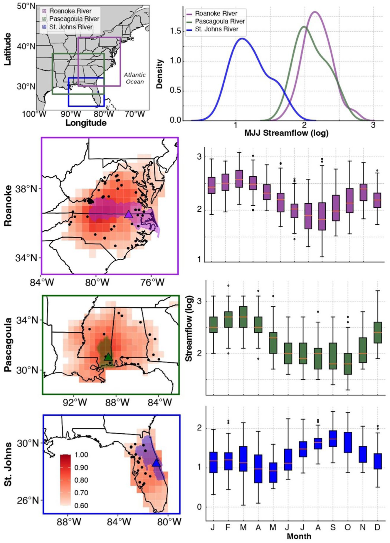
Study area, gauges, predictor network, and hydroclimatology. Top-left: regional map with the three analysis domains (Roanoke—purple; Pascagoula—green; St. Johns—blue) and gauge locations (colored triangles). Top-right: kernel densities of log-transformed May–July (MJJ) streamflow for each gauge (USGS NWIS; retrieved with dataRetrieval). Rows (Roanoke, Pascagoula, St. Johns): left panels show each gauge’s “drought footprint” used for screening predictors—SPEI correlations with MJJ streamflow (threshold ⩾ 0.6; darker reds corresponding to stronger correlations; SPEI from Vicente-Serrano et al. (2010; fields from KNMI Climate Explorer; Trouet and Van Oldenborgh, 2013). Black points are tree-ring chronology sites retained from the ITRDB and unpublished collections; colored triangle marks the gauge; colored polygons indicate the boundaries of the hydrologic unit subregion extent for the respective river. Right panels show monthly distributions of log streamflow (1934–2022); boxes span the interquartile range with medians, whiskers to 1.5×IQR, and outliers shown as points.

Tree-ring data and reconstruction

We compiled tree-ring data from 287 sites across the SAG to form the predictor pool for reconstructions (Supplemental Table 1). Data were obtained from both the International Tree-Ring Data Bank (Zhao et al., 2019) and from unpublished data sets. All samples were previously (i) prepared using standard dendrochronological techniques (Stokes and Smiley, 1968), (ii) visually and statistically cross-dated in standard dendrochronological programs such as CooRecorder (v8.1; Maxwell and Larsson, 2021), and (iii) quality-controlled using the program COFECHA (Holmes, 1983). The initial predictor pool included 290 chronologies, including chronologies of total ring width, earlywood width, and latewood width, from 31 different species. Chronologies spanned the years 604 BCE to 2023, with an average chronology length of 359 years (standard deviation = 307 years).

In dendrochronology, detrending is used to remove trends associated with wood formation over an expanding circumference (i.e. age-related growth trend), while preserving as much information related to the variable being reconstructed. To avoid introducing temporal bias in our reconstruction, particularly the loss of low-frequency variability near the present (Klesse, 2021), we did not apply standard detrending methods such as the 2/3-n spline (Cook, 1985). Instead, each ring width series was detrended using a 100-year fixed-length spline with a frequency cutoff of 0.5 to ensure variance preservation was consistent across time. Given the wide-ranging lengths of standard chronologies forming the predictor pool (60–2622 years, x ¯ = 359 years), use of a fixed spline avoids having to make a priori assumptions about the shape of the growth curve (e.g. negative exponential) while maintaining consistent power to resolve low-frequency trends (Klesse, 2021). All detrending was performed in the R package dplR (v1.7.7).

The climate footprint approach was used to screen chronologies suitable for each reconstruction (Maxwell et al., 2017a). This approach ensures reconstructions only include those chronologies that responded to similar hydrologic conditions as our target basin and ensures each predictor appears in only one reconstruction (Maxwell et al., 2022). Using KNMI Climate Explorer (Trouet and Van Oldenborgh, 2013; http://climexp.knmi.nl) we performed a field correlation between May and July observed streamflow and gridded 0.5° Standardized Precipitation Evapotranspiration Index (SPEI) at a 3-month time step ending in July (i.e. July SPEI-3) for the time period common to all time series (1934–2018). SPEI is a commonly used drought index that uses precipitation and potential evapotranspiration data to estimate drought conditions and, unlike other drought metrics, can be calculated at multiple time scales (Vicente-Serrano et al., 2010). Although meteorological drought often has a wider spatial footprint than hydrologic drought (Hisdal and Tallaksen, 2003), hydrologic drought arises from meteorological drought and so is a reasonable approximation for the climate footprint. The results of each SPEI-streamflow correlation were a series of nested rasters showing the spatial distribution of particular correlation strengths (e.g. R ≥ 0.50, R ≥ 0.60, etc.). We used the raster corresponding to R ≥ 0.60 (p < 0.01) to filter our chronologies such that all chronologies intersecting this raster were kept in the predictor pool for that particular gauge. The R ≥ 0.60 threshold was chosen to maximize the predictor pool for each reconstruction while simultaneously ensuring that predictor pools for each reconstruction were independent (Supplemental Figure 9). These drought footprints largely overlapped with the streamflow clusters identified by McCabe GJ and Wolock, (2014), confirming the footprint captured hydrologic variability in each cluster while ensuring independent predictor pools for each reconstruction (Figure 1). This spatial filter reduced the number chronologies in the predictor pool for each reconstruction to 97 in the SA (19 species), 31 in the SMRB (7 species), and 35 in the NCF (5 species).

Streamflow reconstructions were performed using point-by-point regression (Cook et al., 1999) with the PPR program (v10/09/2019). As designed, this program performs nested, principal component regression of gridded climate fields (e.g. drought). The predictor pool of tree-ring chronologies is first filtered by a user-specified distance from each grid point and the number of chronologies in the predictor pool is further reduced based on the correlation strength between the tree-ring chronology and the climate variable of interest. For a chronology to make it past this stage it must be significantly correlated (p < 0.1, one-tailed) to climatic data according to Pearson’s R, Spearman’s Rho, and the Robust Pearson statistic.

For our analysis we use a simplified version of PPR that performed reconstructions at a single grid point (i.e. streamflow gauge) rather than on a gridded climate field. Rather than utilize PPR’s distance screening, chronologies were screened based on the previously mentioned climate footprints. This ensures that only those chronologies reasonably expected to respond to regional hydrological patterns are included in the reconstruction. We did still utilize PPR’s statistical screening to select for chronologies that contained a May-July streamflow signal. Although an individual tree-ring site may not have a direct hydrologic connection to the reconstructed river, chronologies that pass both the spatial and statistical screening are likely responding to the same climatic factors (e.g. precipitation, evapotranspiration) that regulate summer streamflow in the region. Although there are additional factors (i.e. drainage area, pathways of water transport) that also regulate discharge, this approach provides a reasonable estimate of historical discharge.

We reconstructed May-July discharge at each streamflow gauge based on the period common to all gauges (1934–2022). To ensure the reconstruction was adequate and models were not overfitted, we verified our reconstructions using split validation. To do this, each discharge record was split into the following calibration and verification periods: Roanoke (calibration = 1971–1991, verification = 1934–1970), Pascagoula (calibration = 1965–1992, verification = 1934–1964), and St. Johns (calibration = 1965–1992, verification = 1934–1964). Within the PPR program, the principal components of the selected tree-ring chronologies were regressed against the calibration period, producing a reconstruction. The resulting reconstruction was then verified on the validation period. To assess the skill of the reconstruction, we calculated both the reduction of error (RE) and coefficient of efficiency (CE) (Cook et al., 1999, Appendix B). RE[CE] compares each observed value in the calibration[verification] period to both the reconstructed value and the mean value of the calibration[verification] period to determine if the reconstruction is a better fit of the observed data than simply using the mean of the calibration[verification] period. The final reconstructions are based on the regression between the entire observed discharge record and the principal components of tree-ring chronologies.

In order to assess the relative contribution of each chronology and species on the final reconstruction, we performed an analysis of the standardized regression coefficients, or beta weights (Maxwell et al., 2017a). Beta weights indicate the explanatory power of each model predictor (i.e. chronology), where larger values indicate predictors with more explanatory power. By summing these values for a particular species and dividing it by the sum of beta weights for all predictors we can then estimate each species’ importance to each reconstruction.

Hydrologic drought synchrony

For each reconstruction we identified years over the common reconstructed record with low- (flows at or below the 10th percentile) and high-flow (flows at or above the 90th percentile). The lists of years for each reconstruction were then compared to find years where two or more reconstructions showed an extreme hydrological drought or surplus. To understand changes in reconstruction correlations through time we also calculated 50-year running correlations for each pair of reconstructions. Fifty-year windows provide adequate sample size for identifying significant Pearson correlations while maximizing the temporal resolution.

To investigate changes in hydrologic synchrony with time, we performed Quasi-Poisson regression (Cameron and Trivedi, 2013). The full reconstructed period was separated into four 230-year intervals (1100–1328, 1329–1557, 1558–1786, 1787–2016). For each interval the occurrence of synchronous low- and high-flows was tallied (a) for all basins, and (b) for each pair of basins. Quasi-Poisson regression was performed instead of Poisson regression due to overdispersion and underdispersion in our data (dispersion values for each of the eight combinations of basins and wet/dry periods ranged from 0.345-3.38). Poisson regression was performed using the glm() function in R (R Core Team, 2025).

Severity-duration analysis and return intervals

We performed a severity-duration analysis on each reconstruction to identify the most severe and long-lasting low-flow and high-flow events over the reconstructed record. To do this, we first identified years where streamflow fell above and below the mean value of the reconstruction and for each year calculated the difference between streamflow in that year and the mean streamflow for the entire record (the residual). In order to account for differences in mean river discharge and facilitate comparisons between basins, residuals were normalized by the reconstruction mean. Consecutive years above or below the mean value were placed into groups. The severity of an event was estimated by summing the annual departure from the mean value for group. The duration of an event (j) was the number of years in each group, and the intensity calculated by dividing the severity by the duration (González and Valdés, 2003; Harley et al., 2024). Mathematically, the calculations appear as follows:

Intensity: Severity/Duration where i is an individual year, j is the number of years in the event, and x is the streamflow value. To estimate the occurrence with which we would expect low- and high-streamflow events, we calculated return intervals. For each reconstruction, we split streamflow values into values above and below the mean. The return interval was estimated for low- and high-flow events separately using the Weibull equation (Gumbel, 1941; Makkonen, 2006):

T = ( n + 1 ) / m ,

where T is the return interval, n is the number of low- or high-flow events, and m is the rank of a particular low- or high-flow event.

Spatial patterns of drought

After identifying lows and high-flow events, we mapped the spatial extent of drought and wetness using observed and reconstructed self-calibrated Palmer Drought Severity Index (scPDSI) fields (Dai et al., 2004). scPDSI estimates soil-water balance by accounting for precipitation, evapotranspiration, and local climatology. To enable direct comparison between reconstructed and observed conditions across the SAG, we use scPDSI rather than SPEI, noting that both indices are strongly correlated over the region (r = 0.51; Supplemental Figure 10) and that millennial reconstructions are available only for scPDSI (Cook et al., 2005). For events since 1901, we downloaded gridded monthly scPDSI NetCDF files and generated May–July composites and maps in R; for pre-instrumental events we used the North American Drought Atlas (NADA; Cook et al., 2005), which reconstructs summer (June–August) scPDSI from a network of moisture- and temperature-sensitive tree-ring chronologies spanning 0 CE to present. Although several predictor chronologies used in our streamflow reconstructions also appear in NADA, these maps still provide a useful depiction of event footprints. All maps were clipped to 75°W–96°W and 24°N–42°N.

Reconstruction and synchronous hydrologic drought

Streamflow reconstructions for each river are significantly correlated with observed streamflow (R > 0.60, p < 0.001) (Figure 2). Values of both RE and CE were greater than zero for all reconstructions, indicating each reconstruction is skillful, performing better than the average streamflow for the calibration (RE_Roanoke = 0.39, RE_Pascagoula = 0.45, RE_{St Johns} = 0.62) and verification (CE_Roanoke = 0.39, CE_Pascagoula = 0.45, CE_{St Johns} = 0.62) periods. R_adjusted was 0.58, 0.63, and 0.51 for Roanoke, Pascagoula, and St. Johns, respectively. The reconstructions were also well correlated with the instrumental data over the full calibration period (Supplemental Figure 11).

OPEN IN VIEWER

Figure 2.

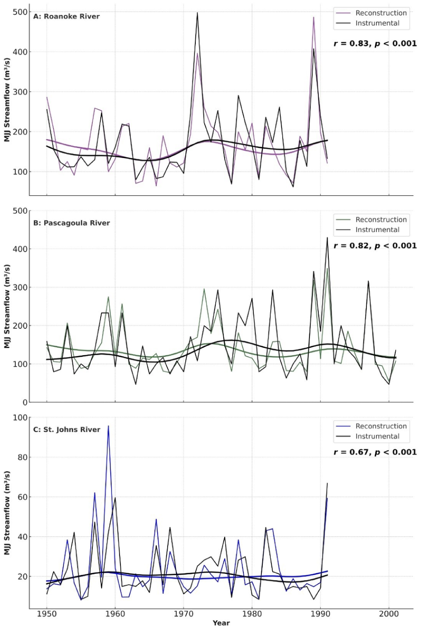
Observed and reconstructed May–July streamflow for (a) Roanoke River, (b) Pascagoula River, and (c) St. Johns River. Reconstructed streamflow (colored lines) is compared to observed (instrumental) records (black lines) at each gauge. Thicker colored and black lines indicate 20-year running means for reconstructed and observed series, respectively. Each panel shows the Pearson correlation coefficient (r) between reconstructed and observed values during the calibration period, with all relationships statistically significant (p < 0.001).

The Roanoke reconstruction extends from 787 to 2022, the Pascagoula reconstruction extends from 907 to 2023, and the St. Johns reconstruction extends from 1089 to 2023 (Figure 3). All reconstructions are truncated to the common period 1100–2015 to simplify comparisons. Average streamflow over the common reconstruction period was 214.7 m³/s (standard deviation = 109.1 m³/s), 140.5 m³/s (standard deviation = 78.3 m³/s), and 19.7 m³/s (standard deviation = 22.6 m³/s) for Roanoke, Pascagoula, and St. Johns respectively. We calculated the relative influence of each chronology based on beta weights (Maxwell et al., 2017a) to determine which chronologies and which species were most important to each reconstruction (Supplemental Figure 12). The Roanoke reconstruction included 13 different species, of which the most important (ranked by relative influence calculated from beta weights) were (Taxodium distichum (L.) (TADI), Quercus alba L. (QUAL), Quercus prinus L. (QUPR), and Tsuga canadensis (L.) Carr. (TSCA). The Pascagoula reconstruction included three species (TADI, Pinus palustris Mill. (PIPA), and Quercus prinus L. (QUPR)) of which TADI had the greatest relative influence by a wide margin. For St. Johns, chronologies from four species were retained in the reconstruction, with PIPA and TADI being the most important, followed by Quercus lyrata Walt. (QULY) and Quercus stellata Wangenh (QUST). The latter emphasizes the ability of PIPA to capture moisture signals in Florida.

OPEN IN VIEWER

Figure 3.

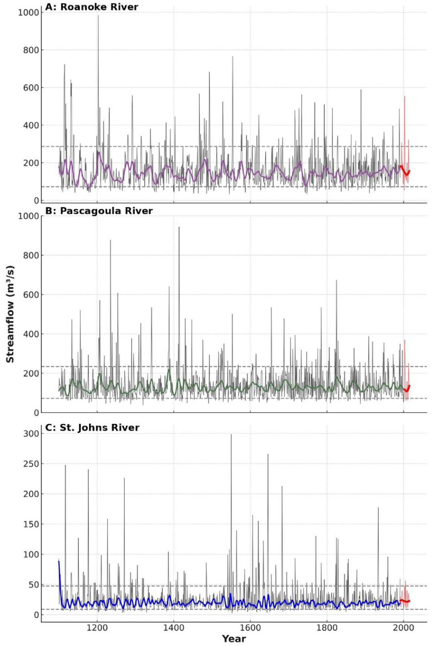
Reconstructed streamflow for the Roanoke, Pascagoula, and St. Johns Rivers (1100–2015 CE). (a) Roanoke River (pink), (b) Pascagoula River (green), and (c) St. Johns River (blue). Solid black lines show annual (May–July) reconstructed streamflow values for each gauge. Colored lines show the 20-year running average, and red segments indicate the instrumental period. Horizontal dashed lines represent the mean reconstructed flow for each record.

Comparing dry (10th percentile and below) and wet (90th percentile and above) years provides a better understanding of shared hydrology across the SE. We identified 41 low-flow and 48 high-flow years that occurred simultaneously in two or more basins (Supplemental Table 2). Of the drought events, most shared drought years were synchronized between the Pascagoula and St. Johns regions (15), followed by Roanoke and Pascagoula (12), and Roanoke and St. Johns (9). We also identified 5 years in which hydrologic drought was shared between all three basins. Shared high-flow years were also most common between Pascagoula and St. Johns (21), followed by Roanoke and Pascagoula (17), and Roanoke and St. Johns (9). In only 1 year (1717) was an extreme wet event recorded in all three reconstructions. Over the entire 916-year period of record, 29% of synchronized low-flow events and 19% of synchronized high-flow have occurred since 1900. Notably, there is an absence of shared extreme dry and wet years between 1800 and 1930.

To quantify the spatial coherence of streamflow extremes across basins, we calculated the odds of co-occurring low or high flows between pairs of rivers. Table 1 shows the odds that a basin is experiencing extreme low flows (⩽10th percentile) [extreme high flows (⩾90th percentile)] given another basin is experiencing low [high] flows. Synchronous hydrologic drought is more likely to occur between the Pascagoula and St. Johns River than between any other combination of rivers. When the St. Johns River is experiencing low [high] flows, there is a 40% [48%] chance the Pascagoula River is experiencing a similarly extreme low [high] flow. In contrast, low [high] flows on the St. Johns River only correspond to low [high] flows on the Roanoke River roughly 29.2% [22.2%] of the time. When the Pascagoula River is experiencing extreme low [high] flows, the Roanoke only experiences extreme low [high] flows about 27.9% [36%] of the time.

OPEN IN VIEWER

Table 1.

Probability of synchronous streamflow extremes among the Roanoke, Pascagoula, and St. Johns Rivers.

(a) Low-flow events
Low-flow river	Roanoke probability low flow	Pascagoula probability low flow	St. Johns probability low flow	All Basins probability low flow
Roanoke	—	26.2	21.5	7.7
Pascagoula	27.9	—	32.8	8.2
St. Johns	29.2	41.7	—	10.4
(b) High-flow events
High-flow river	Roanoke probability high flow	Pascagoula probability high flow	St. Johns probability high flow	All Basins probability high flow
Roanoke	—	31.0	17.2	1.7
Pascagoula	36.0	—	44.0	2.0
St. Johns	12.2	48.9	—	2.2

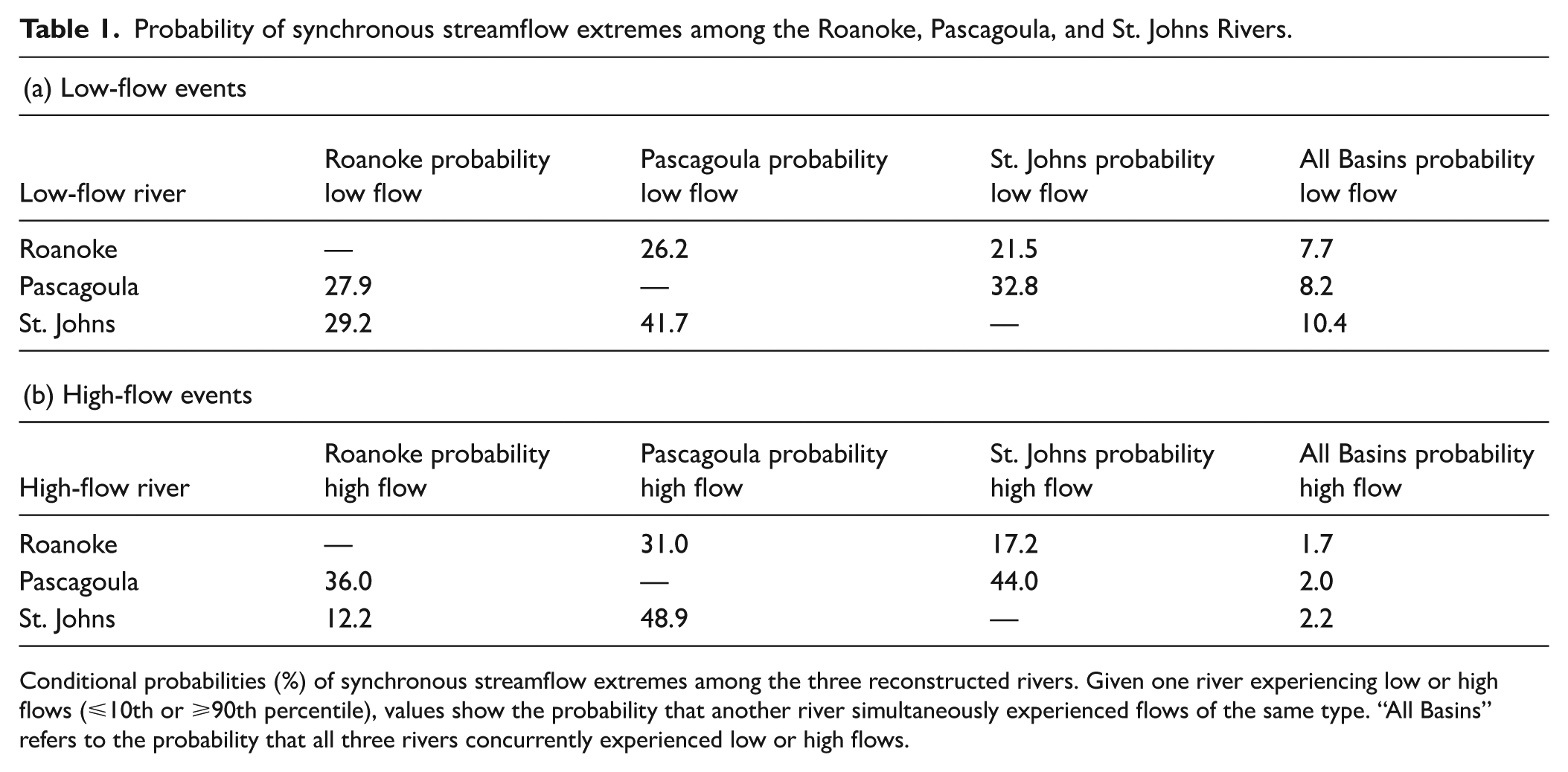
Conditional probabilities (%) of synchronous streamflow extremes among the three reconstructed rivers. Given one river experiencing low or high flows (⩽10th or ⩾90th percentile), values show the probability that another river simultaneously experienced flows of the same type. “All Basins” refers to the probability that all three rivers concurrently experienced low or high flows.

In addition to exploring shared extreme years, we also identified statistically significantly (p < 0.05) correlated periods between gauges (Figure 4b). No pair of gauges were significantly correlated for the entirety of the reconstructed streamflow record. The Pascagoula and St. Johns gauges shared the strongest relationship, with significant correlations observed for almost 1/3 of the record and between 1500 to present. The Roanoke and Pascagoula were significantly correlated for a smaller range of years, particularly since 1900. Unlike the previous pairs, the Roanoke and St. Johns reconstructions are only significantly correlated for short (<50 year) periods.

OPEN IN VIEWER

Figure 4.

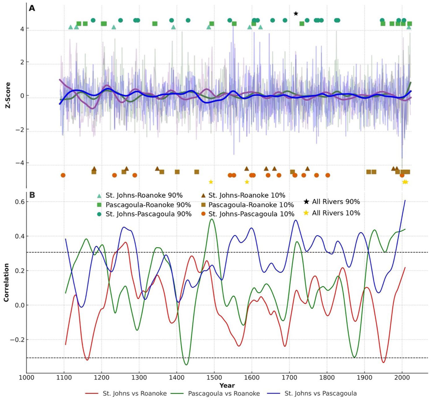
Synchronous low- and high-flow events across the South Atlantic–Gulf region. (a) Reconstructed May–July streamflow (Z-scores) for the Roanoke ( light pink), Pascagoula (light green), and St. Johns (light blue) Rivers, highlighting synchronous extreme events. Thick pink (Roanoke), green (Pascagoula), and blue (St. Johns) lines are 30-year running averages. Symbols mark years when two or more basins experienced concurrent extremes. Shared low-flow (≤10th percentile) events shown with dark brown triangle (St. Johns and Roanoke), light brown squares (Pascagoula and Roanoke), orange circle (St. Johns and Pascagoula), and yellow star (shared event across all three basins). Shared high-flow (⩾90th percentile) events shown with light green triangle (St. Johns and Roanoke), green square (Pascagoula and Roanoke), dark green circle (St. Johns and Pascagoula), and black star (shared event across all three basins). (b) Running 20-year correlations between reconstructed streamflow series for each pair of basins: St. Johns–Roanoke (red), Pascagoula–Roanoke (green), and St. Johns–Pascagoula (blue). Dotted portions of each line indicate statistically significant correlations (p < 0.01).

An increase in frequency of synchrony across two or more basins is not supported by statistical testing (Table 2). None of the eight models identified time as a significant factor in the occurrence of low- or high-flow event synchrony across any combination of basins.

OPEN IN VIEWER

Table 2.

Quasi-Poisson regression and changes in synchrony through time.

(a) Low-flow events
Variable	Roanoke-Pascagoula low flow	Roanoke-St. Johns low flow	Pascagoula-St. Johns low flow	All Basins low flow
Intercept	E = 0.16, SE = 0.89, t = 0.19, p = 0.87	E = 0.46, SE = 0.84, t = 0.55, p = 0.64	E = 0.80, SE = 1.3, t = 0.62, p = 0.60	E = −2.4, SE = 1.1, t = −2.2, p = 0.16
Time period	E = 0.34, SE = 0.29, t = 1.2, p = 0.35	E = 0.13, SE = 0.29, t = 0.46, p = 0.69	E = 0.17, SE = 0.45, t = 0.39, p = 0.74	E = 0.86, SE = 0.31, t = 2.8, p = 0.11
(b) High-flow events
Variable	Roanoke-Pascagoula low flow	Roanoke-St. Johns low flow	Pascagoula-St. Johns low flow	All Basins low flow
Intercept	E = 1.9, SE = 0.44, t = 4.2, p = 0.05	E = 2.1, SE = 0.61, t = 0.35, p = 0.07	E = 1.2, SE = 0.72, t = 1.7, p = 0.24	E = −2.5, SE = 3.5, t = −0.73, p = 0.54
Time period	E = −0.20, SE = 0.18, t = −1.1, p = 0.37	E = −0.67, SE = 0.31, t = −2.2, p = 0.16	E = 0.17, SE = 0.25, t = 0.70, p = 0.55	E = 0.42, SE = 1.1, t = 0.38, p = 0.74

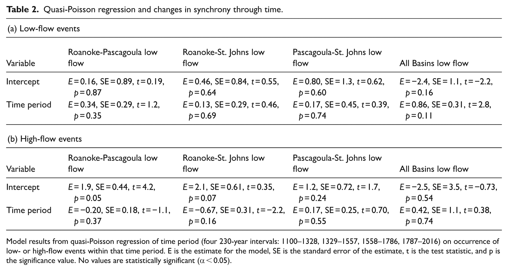
Model results from quasi-Poisson regression of time period (four 230-year intervals: 1100–1328, 1329–1557, 1558–1786, 1787–2016) on occurrence of low- or high-flow events within that time period. E is the estimate for the model, SE is the standard error of the estimate, t is the test statistic, and p is the significance value. No values are statistically significant (α < 0.05).

Severity-duration and return intervals

In the Roanoke basin, above average low and high flows tend to last longer than in the other basins (Figure 5). We identified 183 low-flow events and 182 high-flow events over Roanoke’s reconstructed record. On average, low-flow events last 3.1 years while high-flow events last 2.9 years. After Roanoke, low-flow events last longer at Pascagoula (2.4 years) than at St. Johns (2.2 years), but high-flow events last slightly longer at St. Johns (2.0 years) compared to Pascagoula (1.9 years). Although the Roanoke had longer events on average, the longest low-flow event occurred on the St. Johns River in 1459, lasting 26 years.

OPEN IN VIEWER

Figure 5.

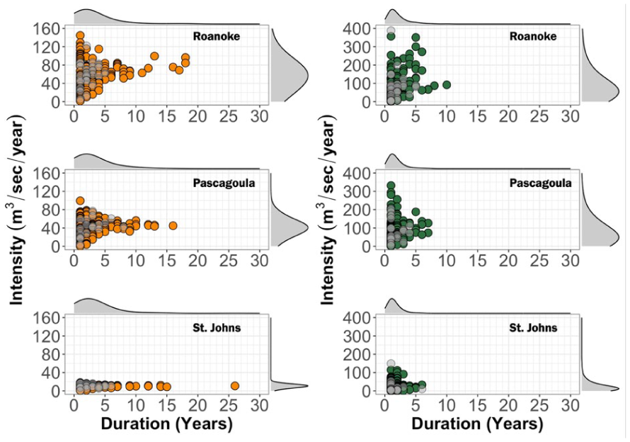
Intensity and duration of drought and pluvial events (1100–2015 CE). Duration and intensity of dry years (left column) and wet years (right column) on the Roanoke, Pascagoula, and St. Johns Rivers. Gray, transparent circles indicate dry or wet events during the instrumental period (Roanoke: 1912–2015, Pascagoula: 1931–2015, St. Johns: 1933–2015). Colored circles indicate dry (orange) or wet (green) events during the reconstructed period (Roanoke: 1100–1911, Pascagoula: 1100–1930, St. Johns: 1100–1932). Gray histograms depict the density distribution of event durations and intensities for each basin.

Although the magnitude of events on the Roanoke River are larger than the other two rivers, the St. Johns River has more intense events based on percentage of annual streamflow. On average, Roanoke streamflow was 81.7 m³/s (62%) less than average for low flow events and streamflow was 56.7 m³/s/year (26%) greater than average for high flow events. In contrast, the average intensity of low-flow [high-flow] events at the Pascagoula and St. Johns were 21.9 m³/s (83%) [10.4 m³/s (54%)] and 68.1 m³/s (27%) [40.4 m³/s (285%)], respectively.

Low-flow return intervals reveal that the low-flow events observed on the Pascagoula and St. Johns are more uncommon than return intervals based on the instrumental record alone would suggest (Figure 6). The most notable example is the low-flow event that occurred on the Pascagoula River in 2000, the lowest flow recorded on this river in either the instrumental or reconstructed record. The instrumental return interval for this event was 60 years, while the reconstructed return interval was 592 years – an order of magnitude difference. Although less extreme, reconstructions along the St. Johns also help put early 2000s low flows in context. For this river the year 2000 had the sixth highest reconstructed return interval at just over 100 years compared to an instrumental return interval of 29.5 years. In contrast, the instrumental period on the Roanoke tends to underestimate the frequency of low flow events. Using the early 2000s again as an example, the lowest flow observed on the Roanoke occurred in 2002 with an estimated return interval of 63 years. In contrast, the reconstructed return interval demonstrates events such as these are more common, with a return interval of 31 years. High-flow events with large return intervals were more common prior to the 20th century, although similar events have occurred in the 20th–21st century.

OPEN IN VIEWER

Figure 6.

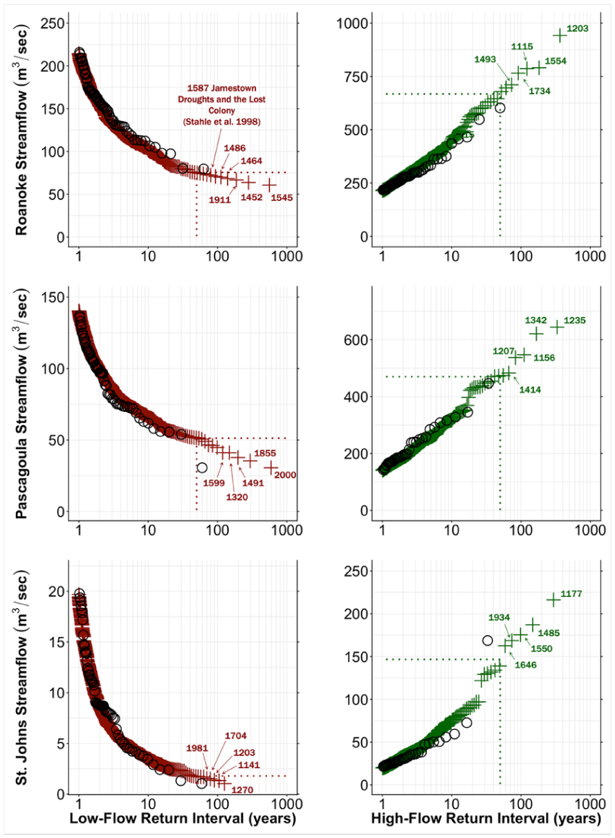
Return intervals of low- and high-streamflow events for common reconstruction period (1100–2015). Red crosses identify low-flow events and green crosses identify high-flow events. Black circles show instrumental period return interval estimates for each river (Roanoke: 1912–2015, Pascagoula: 1931–2015, St. Johns: 1933–2015). Dashed lines indicate 50-year return intervals. Years of selected extreme events are labeled.

Comparisons to observed and reconstructed records

Reconstructions for the Roanoke, Pascagoula, and St. Johns Rivers indicate that observed streamflows are not representative of the multi-century streamflow record. The synchrony observed between Roanoke and Pascagoula River streamflow (McCabe and Wolock, 2014) may not be a consistent hydrological feature in the SE. Despite being significantly correlated over the 20th century, the Roanoke and Pascagoula Rivers have historically not been strongly correlated. In contrast, the Pascagoula and St. Johns River show consistently positive correlations through time. Previous studies relying on the observed streamflow records have disagreed over whether there are two or three streamflow clusters in the SAG. Lins (1997), using observed streamflow from 1941 to 1988, identified only two clusters, a Mid-Atlantic pattern and South Atlantic pattern. Using longer observed records, both McCabe and Wolock (1951–2009) and Rodgers et al. (2020) (1950–2015) identified two distinct streamflow clusters in the South Atlantic, one in north central Florida and one encompassing the Gulf States. Our study shows that the patterns in the NCF and SMRB are strongly correlated for large parts of the record, helping explain why the number of identifiable streamflow clusters changes depending on the record length.

Although this study is far from the first to reconstruct streamflow in the SAG, it does allow for a straightforward comparison of streamflow across the region. Since Cook and Jacoby’s (1983) reconstruction of Potomac River flows, 22 additional streamflow reconstructions have been published on Southeast rivers (Supplemental Table 3). Many of the model predictors used in our reconstructions, particularly from bald cypress (Taxodium distichum), are the same predictors used in these previous reconstructions. As a result, the reconstructions shown here exhibit many of the same long-term patterns as observed in other studies, in spite of differences in reconstruction season and reconstruction length. Additionally, previous studies on tree-ring series synchronization indicates that stressful growing conditions are conducive to tree growth synchronization, especially following extreme climate events (Gazol et al., 2020; Jia et al., 2024; Liang et al., 2003; Shestakova et al., 2016). While the sites in this study are not necessarily located in a region that is stressful to tree growth (i.e. the SAG is relatively warm and wet with a long growing season), synchrony in our results does increase following extreme droughts and pluvials. These studies also support our result that synchrony is high in the most recent century of analysis.

The only other regional reconstructions of streamflow for the SAG also agree with our findings as we would expect given the overlap in chronologies. Ho et al. (2017) reconstructed streamflows over the past 500 years for the entire continental US, including the SAG. This work found SAG streamflow either exhibited no trends or decreased toward the present, and the lack of a long-term trend in our reconstructions reaffirms the former. The work of Maxwell et al. (2017a) investigated the synchrony of streamflow across the East Coast and found that streamflow in the Mid-Atlantic region behaved as a hinge, occasionally correlated to activity in northern rivers and at other times correlated to activity in southern rivers. This is consistent with our observations that the similarities between Roanoke and Pascagoula streamflow are limited to the observed streamflow record. During the remaining time the Roanoke River is likely more in-sync with rivers farther north.

While other paleohydrologic proxies exist in the region, their coarse temporal resolution and limited spatial extent makes comparison to our current work challenging. Still, one comparison that can be made offers tentative support for the validity of our reconstructions. Late-Holocene precipitation reconstructed from δ¹⁸O speleothem records in Alabama generally align with low-frequency variability in reconstructed Pascagoula streamflow. Both reconstructed summer streamflow and (primarily) summer precipitation indicate wetter conditions between the mid-1100s to mid-1500s, with a shift from wetter to drier conditions beginning in the mid-1500s (Medina-Elizalde et al., 2022). As Medina-Elizalde et al. note, other tree-ring precipitation reconstructions in the region do not show a similar pattern, which may be because our reconstruction specifically targets summer water availability. Although we found additional paleo-precipitation reconstructions within the Pascagoula region (e.g. Aharon and Dhungana, 2017, Hillman et al., 2024), these did not have adequate temporal resolution to compare to the Pascagoula streamflow reconstruction. While it is clear that tree rings serve as the most abundant proxy for late-Holocene paleohydrology in the region, further development of traditional proxies (e.g. speleothems, lake sediments) or newer proxies (bat guano isotopes (Tsalickis et al., 2024) or Odocoileus virginianus tooth enamel (Bonham, 2023)) will allow for better future comparisons.

Our results also provide greater context for the drought that staggered the southeast US between 2006 and 2008. This drought, resulting in large amounts of environmental (Clark et al., 2008) and economic (Nguyen et al., 2023) damage, spurred calls for a drastic paradigm shift in southeastern water management (Manuel, 2008; NIDIS, 2022). Tree-ring based drought reconstructions for the Appalachicola-Chattahoochee-Flint basin, one of the basins hardest hit by the drought, found that droughts like that which occurred in 2006–2008 are unremarkable in the 346-year paleorecord (Pederson et al., 2012). Our severity-duration analysis supports this finding, as the 2006–2008 drought’s intensity and duration did not stand out compared to other drought events. The spatial extent of the 2006–2008 drought, however, was unique. Out of the 5 years where synchronized hydrologic drought occurred over the entire SAG, two of those years were in 2006 and 2007. This suggests that the 2006–2008 drought was remarkable largely for its spatial coverage (Figure 7). Although droughts spanning the entire SAG are rare, three of the five region-spanning events have occurred since 2000, which should be a concern for water managers in the region.

OPEN IN VIEWER

Figure 7.

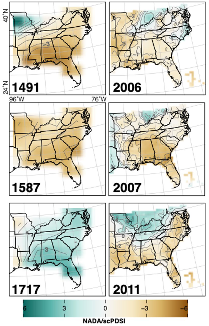
Spatial patterns of synchronous drought and pluvial events across the Southeast Atlantic–Gulf region. Maps depict May–July self-calibrated Palmer Drought Severity Index (scPDSI) anomalies for years of synchronous extreme flow identified in the streamflow reconstructions. Left panels (1491, 1587, 1717) show reconstructed drought and pluvial conditions from the North American Drought Atlas (Cook et al., 2005). Right panels (2006, 2007, 2011) show observed scPDSI fields generated using the KNMI Climate Explorer. The scPDSI integrates both precipitation and evapotranspiration to estimate soil moisture balance and is presented here instead of SPEI to facilitate comparison with reconstructed records. Each map is limited to the region spanning 76°–96° W and 24°–40° N. Historic droughts (1491, 1587, 2011) exhibit strong coastal drying with weakening inland gradients, whereas the 2006–2007 droughts were centered over Alabama and Georgia.

Hydrologic drought risk in the SE

Synchronous hydrologic droughts across the SAG are rare, but if they were to occur they would be damaging to the environmental and economic health of the region. Over the last 936 years, we found just five drought events that were synchronized over the entire SAG, with three of these events occurring in a 6-year span during the 21st century. Both the 2006 and 2007 synchronous drought years were part of the infamous 2006–2008 drought that crippled the SE. Unusually low precipitation across the region made 2007, at the time, the second driest year on record for the SE. The result was losses to major field crops totaling more than $1.3 billion, power companies being forced to switch from thermoelectric power to fossil fuels, wide-spread forest mortality, increased wildfires, and a state of emergency in Atlanta after being only a few months away from running out of drinking water (Clark et al., 2008; Ding et al., 2007).

While full SAG-wide synchrony is uncommon, partial synchrony involving two basins is substantially more frequent and represents an important regional-scale hazard. We identified 36 years in which low flows occurred simultaneously in two basins, indicating that multi-basin drought impacts are not anomalous but a recurring feature of the hydroclimatic record. These events were evenly distributed throughout the reconstructed period. When one river experienced low flows, there was an 8–10% probability that at least one additional basin also experienced low flows. Such levels of synchrony have meaningful implications for regional water supply reliability, as concurrent low flows can limit opportunities for inter-basin buffering or adaptive management.

Synchrony was particularly strong between the St. Johns and Pascagoula Rivers, suggesting that these basins function as a coherent hydrologic cluster during drought conditions. This relatively consistent relationship highlights the need for coordinated drought planning and management within these systems. Given the geographic proximity of the Pascagoula and St. Johns Rivers to ongoing legal conflicts over streamflow allocation (Bearden and Andreen, 2017), improved understanding of partial synchronous droughts may be especially valuable for informing drought preparedness, water-sharing agreements, and contingency planning.

The spatial form and extent of synchronous hydrologic drought across all basins can vary considerably between years (Figure 7). Years of synchronous drought include 1491, 1587, 2006, 2007, and 2011. Droughts in 1491, 1587 and 2011 each show a similar pattern where intense droughts were restricted to coastal states and drought severity decreased moving inland. The 2006 and 2007 drought years both exhibit a distinct form. The 2006 drought was much more severe for the Gulf states, with wetter conditions moving up along the east coast. In contrast, Alabama and Georgia were the epicenter of the 2007 drought with drought severity decreasing as you moved farther from these states. The lone shared high-flow year in 1717 reveals that while the wettest regions were those including the reconstructed rivers, the entirety of the east experienced wet conditions.

Our study provides a much-needed perspective on the spatial and temporal components of hydrologic drought synchrony with the SAG. There is strong interest in synchronous droughts across the world, as such droughts threaten food and water supplies, and, by extension, societal order (Gaupp et al., 2020; Mahto and Mishra, 2023). To date, there has not been such a study conducted for the SAG. Although synchronous drought is a common topic in the literature, this work is unique for the type of drought explored, its temporal extent, and, most importantly, its spatial scale. Most investigations of drought synchrony focus on meteorological rather than hydrological drought (e.g. Mondal et al., 2023; Zhao et al., 2024), often employing drought indices such as SPEI or scPDSI. While these are equally important, the relationship between meteorological and hydrologic drought is not always linear, so having information on hydrologic drought can be more immediately helpful to water managers. The research that does focus on hydrologic drought synchrony can be classified into studies that utilize dense networks of observational streamflow records and those that rely on reconstructed records. While investigations of drought synchrony using networks of streamflow gauges benefit from a higher spatial resolution with which to diagnose drought extent, these records are often short, as little as 35 years (Abdelkader and Yerdelen, 2022; Sharma and Mujumdar, 2024).

By utilizing tree records, studies like this one are able to place hydrologic drought synchrony into a multi-century context. Spatial comparisons of drought are not uncommon in tree-ring based streamflow reconstructions, but they do tend to focus more on lower-frequency coherence across space. For example Martin et al. (2019) investigated hydrologic drought synchrony between basins within the Upper Missouri River Basin and Colorado River Basin on 20- and 60-year timescales. Similarly, Maxwell et al. (2017a) evaluated synchrony across eastern U.S. streamflow reconstructions using 20- and 50-year temporal windows. Still, studies like Chuphal and Mishra (2025) do explore drought synchrony on an annual basis. Although the study employed tree-ring reconstructions only indirectly (via reconstructed values of the (Monsoon Asia Drought Atlas), they reconstructed streamflow across 45 gages that provided finer spatial resolution of drought synchrony across the Indian subcontinent. To ensure a large enough number of independent predictors in each of our reconstructions our spatial resolution is limited to the three basins examined, highlighting a limitation of this work.