First Younger Dryas-Early Holocene varve chronology of the Russian Plain

Abstract

Annually-laminated lake sediments (varves) are among the most reliable archives for high-resolution paleoenvironmental reconstruction. However, the Russian Plain has remained a gap in the global distribution of varve chronologies. This preliminary study presents the first Younger Dryas Early Holocene varve chronology from Lake Kasplya (western part of the Russian Plain). A 17.3 m sediment core (Kas-17) was retrieved in 2022, of which the 9.6–15.2 m interval revealed well-preserved biochemical varves. Thin-section microscopy and diatom identification confirmed the annual nature of laminations. Independent chronologies were developed through manual varve counting, and radiocarbon dating. The results indicate a floating varve chronology of 4745 ± 325 annual layers (with cumulative uncertainties of 6.84%), spanning ca. 12.1–7.4 ka BP. Anchoring to radiocarbon age-depth models demonstrates a high level of agreement, with discrepancies within 10%. This record from Lake Kasplya provides a high-resolution terrestrial archive for the Russian Plain and underscores the potential of similar lakes to provide varve-based reconstructions of paleoclimate.

Keywords

palaeolimnology radiocarbon dating varve chronology thin sections diatoms younger Dryas Holocene

Introduction

Varves act as key archives for reconstructing Quaternary paleoenvironmental variability, including ecosystem dynamics, climatic oscillations, and abrupt events (e.g. Brauer et al., 2008; Dräger et al., 2017; Sirocko et al., 2021). Their principal advantage is the presence of an independent varve chronology, providing annual to seasonal resolution (Ojala et al., 2012).

One of the mixed varve types, common for the Holocene, is biochemical varves which consist mostly of organic matter with minerogenic contributions from catchment erosion and autogenic mineral precipitation (Zolitschka et al., 2015). Despite their structural complexity, biochemical varves are widely used for constructing varve chronologies for example, Lake Suigetsu (Nakagawa et al., 2012), Holzmaar (Zolitschka, 2007), Lake Żabińskie (Żarczyński et al., 2018), Elk Lake (Anderson et al., 1993).

The Russian plain (part of the East European Plain, EEP) and the Asian part of Russia are misrepresented in terms of varve chronologies. The worldwide distribution of varved records from the VARDA (Ramisch et al., 2020) reveals a substantial gap extending from the Carpathians to Kamchatka. Existing studies are limited and geographically scattered. Clastic-organic varves have been documented in the Caucasus (Lake Donguz-Orun; Alexandrin et al., 2018) in the Russian Arctic (Lake Bolshoye Shchuchye; Regnéll et al., 2019), and in Siberia (Teletskoe and Shira lakes; Kalugin et al., 2013; Rudaya et al., 2016).

Varved sediments are expected in lakes within the north-western Russian plain, comparable to those in northeastern Poland (Tylmann et al., 2013). One such archive, Lake Kasplya, was identified in 2022. Although the lake is currently shallow and holomictic, its sedimentary infill contains 5.6 m of thin-laminated deposits, making it a unique terrestrial archive for the EEP.

This study aims to confirm the varved nature of the thin-laminated deposits in Lake Kasplya and establish a reliable varve chronology. As the study is currently in its pilot phase, the presented conclusions should be regarded as preliminary.

Study area

Lake Kasplya is located 35 km northwest of Smolensk (54°57′51″N 31°35′51″E, 160.4 m asl; Figure 1(a)–(d)). It is the source of the Kasplya River, a tributary of the Daugava River, and receives inflow from the Klets River. The catchment area (585 km²) lies entirely within the Late Valdai (Weichselian) glaciation zone (Astakhov et al., 2016).

Figure 1.

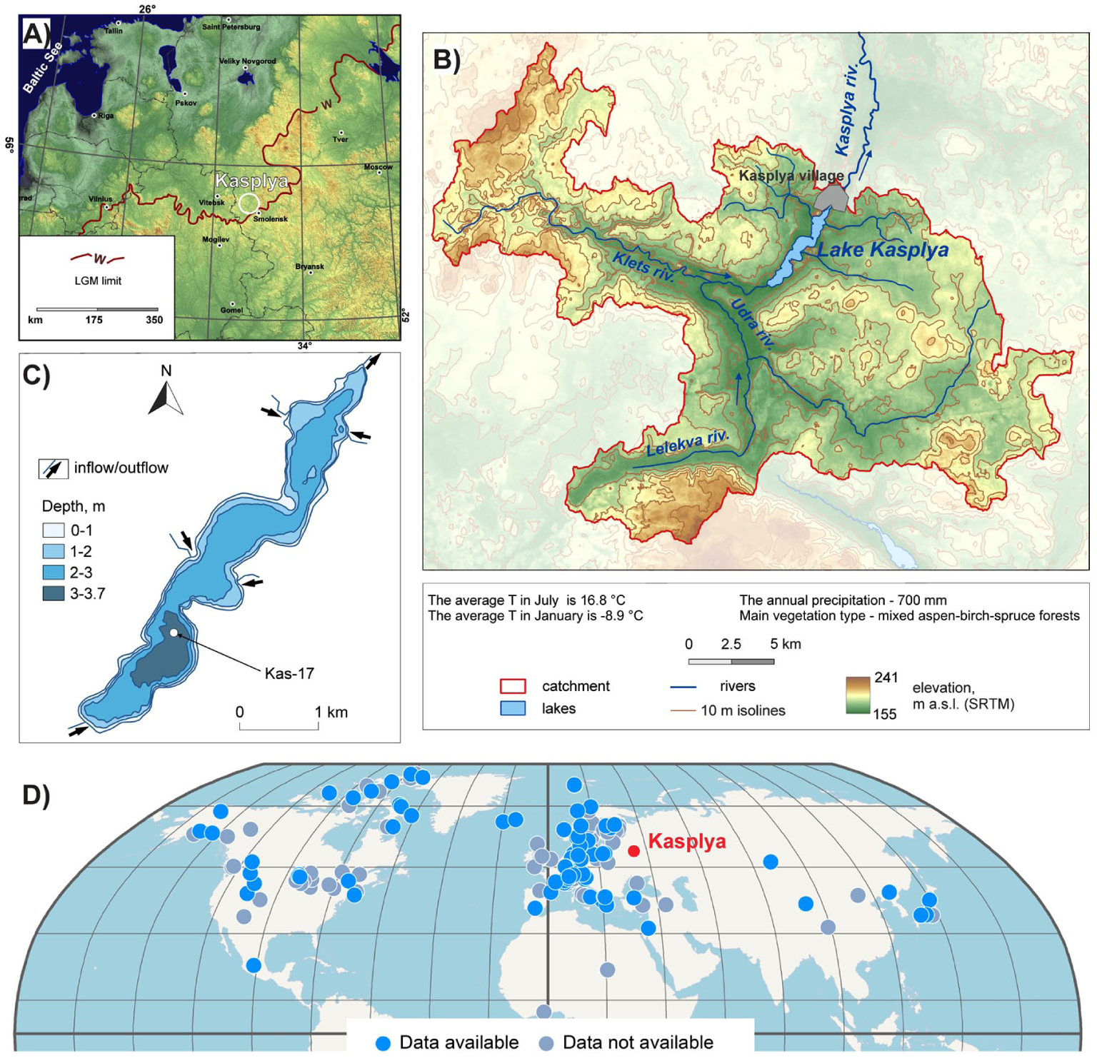
Location of studied area. (a) Lake Kasplya within the East European Plain and LGM margin (Astakhov et al., 2016). (b) Topography of Lake Kasplya’s catchment area. (c) Bathymetric map of Lake Kasplya with the location of the coring site. (d) A fragment of the map “Spatial distribution of identified lakes and collected datasets included in VARDA 1.0.” (Ramisch et al., 2020) with the location of Lake Kasplya.

Lake Kasplya has a surface area of 3.2 km², an elongated southwest–northeast orientation, and a maximum depth of 3.7 m. Its shores are steep and locally terraced, particularly along the eastern margin. The northern shores are marked by terminal moraine ridges composed of till, whereas the southern shores are mainly composed of sandy glaciofluvial deposits (Shkalikov, 2005). Pre-Quaternary rocks lie at altitudes of 130–150 m abs. They represent the deposits of the Famennian stage of the Devonian system: dolomites, limestones, marls, and clays (Stolyarova and Konstantinova, 1972). The basin likely formed through glacial erosion and subglacial meltwater activity (Shkalikov, 2005). Today, the lake is mesotrophic with a tendency towards eutrophication.

Materials and methods

Fieldwork

Sediment cores were retrieved in February 2022 from an ice-covered lake. A bathymetric survey was conducted in the summer of 2023 using a Deeper Pro+ echo sounder.

Coring was performed using a Livingston piston corer with a 100 × 5 cm barrel. The total length of the recovered sediment is 17.3 m. Here we present the results covering the middle part of the profile, 9.6–15.2 m (six cores), which is characterised by rhythmic thin lamination. Below 8 m depth, end-to-end drilling resulted in partial sediment loss, and most cores were shortened to 70–90 cm. We assume the main reason for core shortening is bypassing, which is described for piston corers. Excessive internal resistance within the core barrel can result in the cutting edge becoming blocked and underlying sediments being excluded, meaning that some strata are bypassed and not recovered (Morton and White, 1997).

Laboratory analyses

All Kas-17 cores were split lengthwise, photographed and subsampled in the Laboratory of Environmental Paleoarchives of the Institute of Geography RAS. High-quality (40–50 pix/mm) photographs are presented in Supplemental Material 1.

Loss on ignition

Loss on ignition (LOI) was determined using the stepwise ignition at 550°C and 950°C (Heiri et al., 2001). According to the method of Dean (1974), the percentage of calcite (CaCO₃) was estimated from LOId950/0.44.

Thin section

Preparation of thin-sections consisted of several stages: (1) cutting a sediment block measuring ca. 2 × 4 cm from the core; (2) low-temperature (~22°C) slow drying for 7 days; (3) freeze-drying for 12 h; (4) impregnating the sediment block with epoxy resin; (5) preparation of a 30 µm thin-section using cutting and polishing machines.

Varve structure description

Four thin-sections were examined using the MEKOS-C2 scanning microscope with magnification 40×. Scan images allowed to distinguish sublaminae within the varved section based on: colour, fraction of organic and clastic detritus, fraction of diatoms, and fraction of authigenic minerals (Supplemental Material 2).

In order to obtain more accurate information about the taxon of diatoms, the slides for the light microscopy from the same intervals as thin-sections were prepared using a standard technique for lake sediments (Battarbee et al., 2001). The taxonomic identifications using the microscope Motic BA300 at 1000× magnification were conducted in accordance with Krammer and Lange-Bertalot (1986, 1988, 1991a, 1991b).

Radiocarbon dating and C, N measurement

Radiocarbon dating was made using the liquid scintillation (LSC) and the accelerator mass spectrometry (AMS) methods.

AMS dating was performed at the Shared Research Facility “Laboratory of Radiocarbon Dating and Electron Microscopy” of the Institute of Geography RAS in collaboration with the Centre for Applied Isotope Studies at the University of Georgia, USA. All the samples (17) were dated with the use of the total organic carbon (TOC) fraction due to the absence of visible terrestrial macrofossils and prepared and measured following the procedure described in (Zazovskaya et al., 2017).

LSC dating was performed at the Laboratory of Geomorphological and Palaeogeographic Studies of Polar Regions and the World Ocean, Institute of Earth Sciences, St. Petersburg State University. All the samples (6) were prepared and measured following the procedure described in Arslanov (1987).

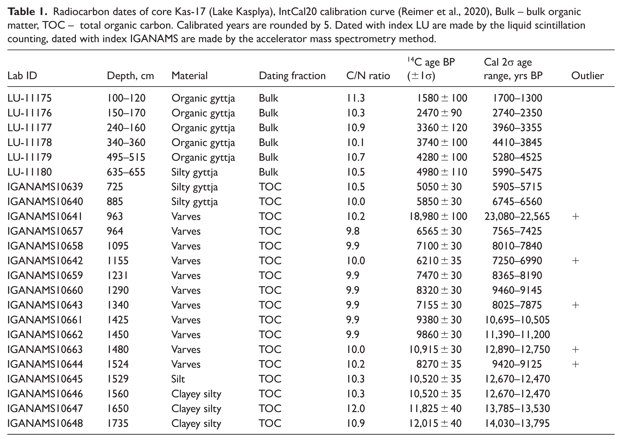
The dates were calibrated using the IntCal20 calibration curve (Reimer et al., 2020). The results are presented in Table 1. The age-depth model was constructed using the rBacon package (v3.1.1), based on Bayesian statistics (Blaauw and Christen, 2011), in the R software (v4.3.2).

Table 1

Radiocarbon dates of core Kas-17 (Lake Kasplya), IntCal20 calibration curve (Reimer et al., 2020), Bulk – bulk organic matter, TOC – total organic carbon. Calibrated years are rounded by 5. Dated with index LU are made by the liquid scintillation counting, dated with index IGANAMS are made by the accelerator mass spectrometry method.

Lab ID	Depth, cm	Material	Dating fraction	C/N ratio	¹⁴C age BP (±1σ)	Cal 2σ age range, yrs BP	Outlier
LU-11175	100–120	Organic gyttja	Bulk	11.3	1580 ± 100	1700–1300
LU-11176	150–170	Organic gyttja	Bulk	10.3	2470 ± 90	2740–2350
LU-11177	240–160	Organic gyttja	Bulk	10.9	3360 ± 120	3960–3355
LU-11178	340–360	Organic gyttja	Bulk	10.1	3740 ± 100	4410–3845
LU-11179	495–515	Organic gyttja	Bulk	10.7	4280 ± 100	5280–4525
LU-11180	635–655	Silty gyttja	Bulk	10.5	4980 ± 110	5990–5475
IGANAMS10639	725	Silty gyttja	TOC	10.5	5050 ± 30	5905–5715
IGANAMS10640	885	Silty gyttja	TOC	10.0	5850 ± 30	6745–6560
IGANAMS10641	963	Varves	TOC	10.2	18,980 ± 100	23,080–22,565	+
IGANAMS10657	964	Varves	TOC	9.8	6565 ± 30	7565–7425
IGANAMS10658	1095	Varves	TOC	9.9	7100 ± 30	8010–7840
IGANAMS10642	1155	Varves	TOC	10.0	6210 ± 35	7250–6990	+
IGANAMS10659	1231	Varves	TOC	9.9	7470 ± 30	8365–8190
IGANAMS10660	1290	Varves	TOC	9.9	8320 ± 30	9460–9145
IGANAMS10643	1340	Varves	TOC	9.9	7155 ± 30	8025–7875	+
IGANAMS10661	1425	Varves	TOC	9.9	9380 ± 30	10,695–10,505
IGANAMS10662	1450	Varves	TOC	9.9	9860 ± 30	11,390–11,200
IGANAMS10663	1480	Varves	TOC	10.0	10,915 ± 30	12,890–12,750	+
IGANAMS10644	1524	Varves	TOC	10.2	8270 ± 35	9420–9125	+
IGANAMS10645	1529	Silt	TOC	10.3	10,520 ± 35	12,670–12,470
IGANAMS10646	1560	Clayey silty	TOC	10.3	10,520 ± 35	12,670–12,470
IGANAMS10647	1650	Clayey silty	TOC	12.0	11,825 ± 40	13,785–13,530
IGANAMS10648	1735	Clayey silty	TOC	10.9	12,015 ± 40	14,030–13,795

The organic carbon (С_org) and nitrogen (N) content were measured by the dry combustion method in CHNS-analyser Vario Isotope Cube (Elementar, Germany) at the Shared Research Facility “Laboratory of Radiocarbon Dating and Electron Microscopy.”

Varve counting and quality assessment

Manual varve counting and thickness measurements were independently conducted by three researchers on high-quality photographs using ImageJ software. By prior agreement, the base of the pale sublayer was used as the most distinct year marker. Missing intervals between cores were interpolated using average varve thickness, assuming a constant sedimentation rate. This rate was calculated as the mean of sedimentation rates at the base of the overlying core and the top of the underlying core (i.e. from both sides of the gap).

As a result, three floating chronologies were obtained. These were combined by calculating the average chronology with uncertainty as the standard deviation (σ) of the individual chronologies, following the approach described by Lamoureux (2001) and referred to as “method B” by Żarczyński et al. (2018). The obtained floating varve chronology was compared with a radiocarbon age-depth model and anchored to the mean modelled calibrated age at a depth of 9.63 m, corresponding to the uppermost level of a clear varved record.

Additionally, a Varve Quality Index (VQI) was determined following Zolitschka (1990) and Bonk et al. (2015a). Groups of layers were assigned to classes of quality: (1) low; (2) high; (3) perfect.

Results

Lithology and age-depth relation

The sedimentary sequence Kas-17 comprises the following sections (Figure 2):

0–7.2 m: dark-brown and olive-brown gyttja, with the highest organic content, low carbonate content; the texture is massive with certain pours.

7.2–9.6 m: faintly laminated silty gyttja with constant organic content and increasing carbonate content; certain light thin laminae occur randomly and increase in number with depth.

9.6–15.2 m: thin-laminated silt, characterised by alternating brown and beige layers, with occasional grey layers interspersed. The content of С_org is 7–10% and the CaCO₃ content varies between 9 and 35% (mean ~20%). A visual inspection of the core surfaces revealed the following: (1) the thickness of the dark-pale pair increases upwards; (2) at a depth of 13.4 m, a distinct transition occurs where laminae become thicker, darker, and reddish after drying; (3) bending and distortion of laminae is only observed at the edges of the cores.

15.2–17.3 m: laminated clayey silt and silt, subdivided into three sublayers of different colours.

Figure 2.

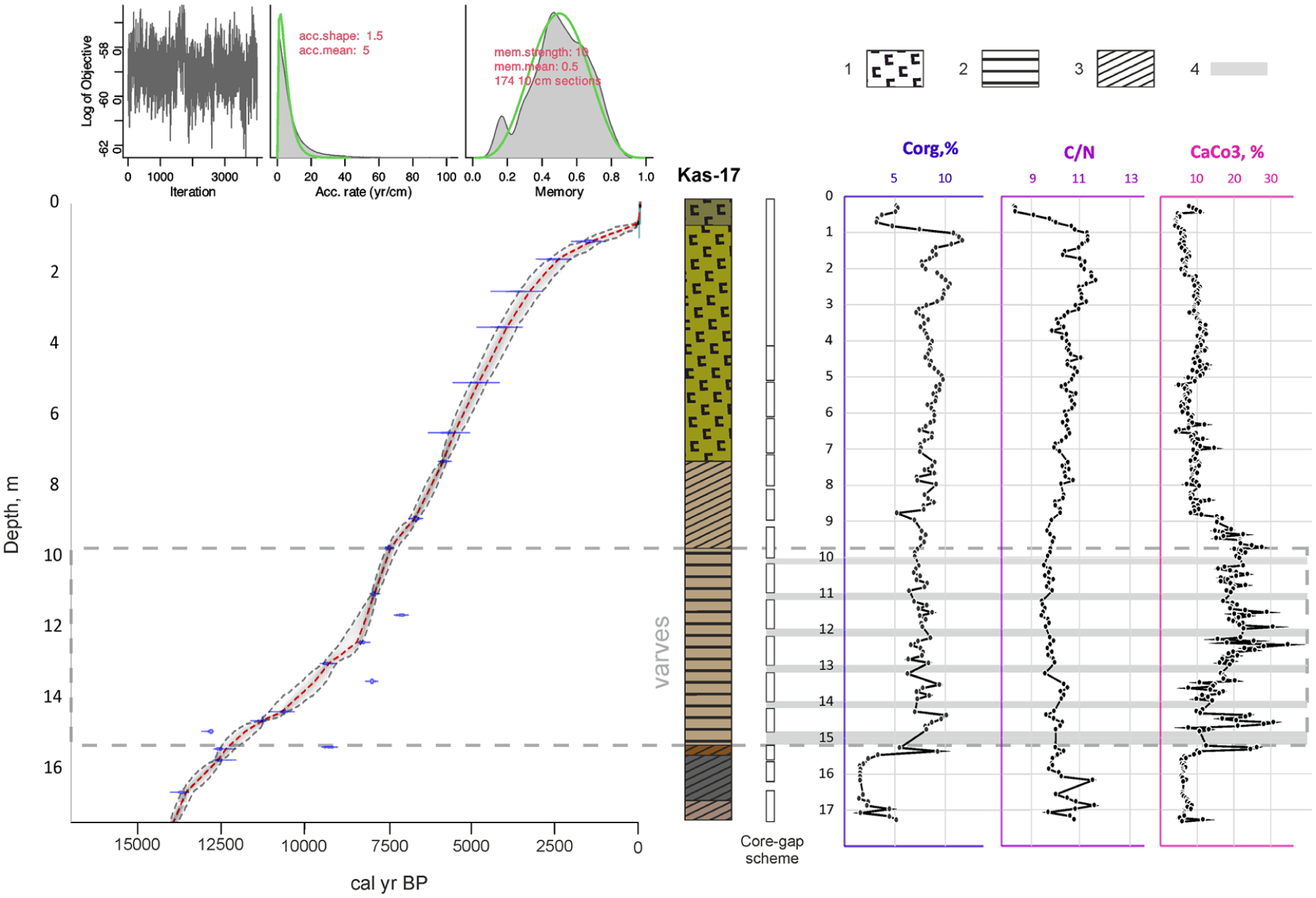
General lithological structure of the sediments of the core Kas-17 and overall age-depth model with the 95% confidence interval made with the use of the rBacon package (Blaauw and Christen, 2011). Lithological description: 1 - gyttja, 2 - varves, 3 - laminated silt, 4 - gaps.

C/N ratios vary from 9.8 to 12.0 throughout the sequence and from 9.8 to 10.3 in the varved section (Figure 2), indicating predominantly autochthonous organic matter and no influence from terrestrial organic matter (based on Meyers and Ishiwatari, 1993).

A radiocarbon age-depth model was built for the overall Kas-17 sequence (Figure 2). Based on this model, the 9.6–15.2 m interval was dated as follows: formation of thin-laminated silt began at 12,057–12,516 (2σ; mean = 12,306) cal BP, and ended at 7178–7501 (mean = 7388) cal BP. A transition between thin-laminated silt types at 13.4 m occurred around 9700 cal BP.

Varve microstructure, thickness, and quality

Fragments of four thin-sections are present in Figure 3. Although minor structural differences occur within individual thin-sections, the overall characteristics of the thin-laminated silt are consistent.

Figure 3.

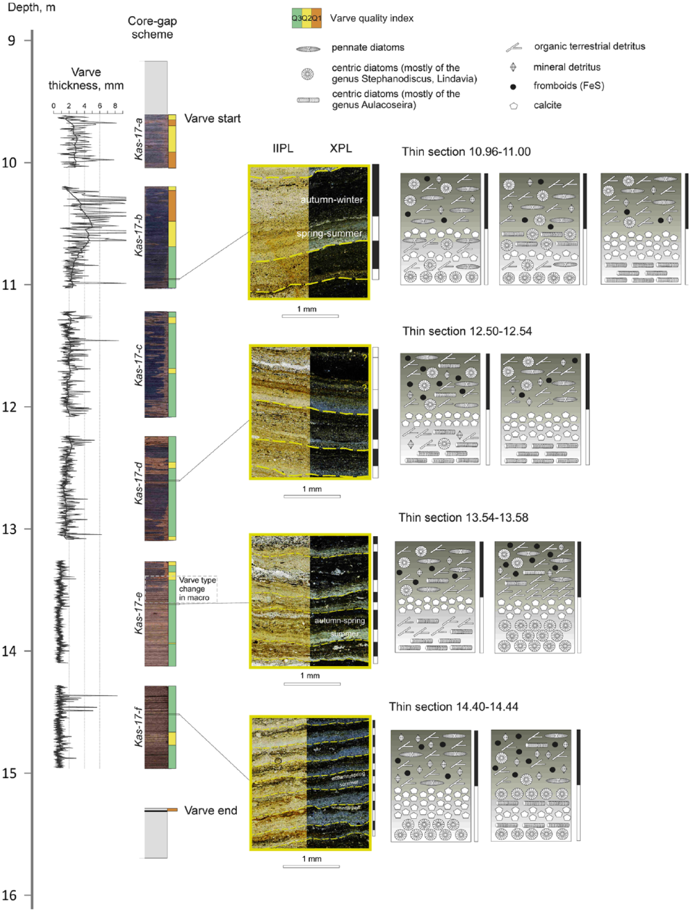
Varve structure, thickness and quality of Kas-17 core. The thickness graph is based on the manual count of MA; the quality data are based on VQI; varve structures are shown with thin section scans in parallel (IIPL) and cross (XPL) polarised light, and schematic structure (varve couplets are indicated by black and white bars). For high-quality photographs of cores see Supplemental Material 1. For full scans of thin sections see Supplemental Material 2.

Below 13.4 m (thin-sections 13.54–13.58 and 14.40–14.44), laminae are thin, averaging 0.7 mm. They consist of a pale lamina made up of a thin diatom sublayer (featuring both pennate and centric species, the latter predominating) and a thicker calcite sublayer, followed by a dark lamina composed of organic matter, minerogenic detritus, and framboids (spherical pyrite crystals).

Above 13.4 m (thin-sections 10.96–11.00 and 12.50–12.54), laminae gradually thicken, averaging up to 1.85 mm, and become more complex in structure. In the pale laminae, diatomite sublayers become thicker, the diversity of diatom frustules increases, and the calcite sublayer becomes thinner or may nearly disappear. Pairs with two diatom sublayers, or mixed diatom-calcite lamina, are frequently encountered. Dark sublayers remain relatively uniform, but show increased organic and reduced mineral content.

Diatom analyses indicate that the annual sedimentation cycle usually involves a predominance of centric diatoms (Aulacoseira spp., Lindavia spp., and Stephanodiscus spp.) preceding the calcite deposition. Above 13.4 m, a second diatom post-calcite sublayer is clearly observed (represented by either pennate or centric diatoms). However, below 13.4 m a second diatom sublayer also appears.

The structure of annual couplets tends to become less complex with depth, and the varve thickness decreases accordingly (Figure 3).

VQI results: Q1 - 9.5%, Q2 - 20.1%, Q3 - 70.4% (Figure 3). Most of the low-quality varves occur in the upper part of the varved layer - 9.6–10.7 m.

Varve counting results and validation with radiocarbon dating

The count of individual layer pairs in the depth interval of 9.6–15.2 m for independent counts without gap interpolation is 3388, 3471, and 3855 pairs. After interpolating missing core sections, the counts increase to 4468, 4563, and 5203, respectively (Figure 4). Counting results differ the most in the depth intervals of 9.6–11 m due to poor varve visibility (VQI = 1–2; Figure 3) and in 14–15.2 m due to the interpolation effect of a large number of varves. The mean count is 4745 ± 325 (uncertainty of 6.84%).

Figure 4.

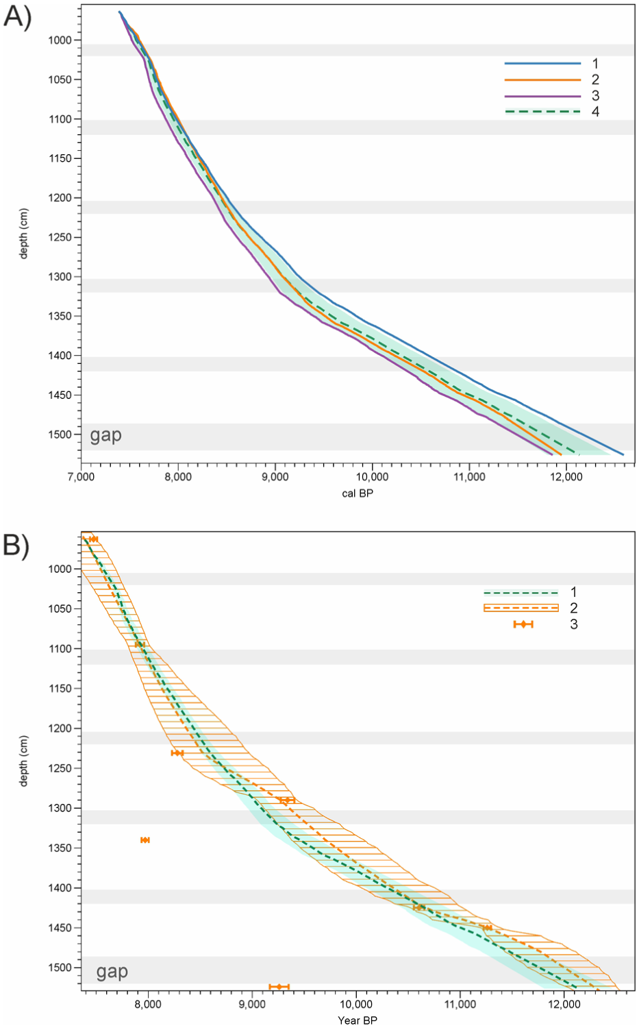
Varve chronology of Kas-17: (a) Individual manual counts of varves (1 - LS, 2 - AZ, 3 - MA) and resultant average varve chronology with standard deviation as a dashed line with colour fill (4) anchored to ¹⁴C modelled age. (b) Comparison of the averaged manual varve chronology (1) with radiocarbon age-depth model with the 95% confidence interval (2) based on ¹⁴C dates (3). Grey bars – gaps between cores.

The floating varve chronology was anchored to the ¹⁴C age-depth model at 7388 cal BP at 9.63 m depth. It’s the topmost of the clear varve and a starting point for counting (Figure 4).

According to the ¹⁴C model, varve formation at 15.26 m began between 12,057 and 12,516 cal BP (mean = 12,306). The anchored varve chronology yields a slightly younger age estimation for the same event - 12,133 ± 325 cal BP. While absolute ¹⁴C uncertainty remains relatively constant, varve-age uncertainty increases cumulatively with depth. Overall, varve and radiocarbon chronologies agree within ~10% (⩽200 years). Agreement is strongest in the uppermost 3 m and the basal metre, with larger discrepancies in the middle section. The consistency between methods confirms the annual nature of lamination and indicates continuous varve formation in Lake Kasplya since the Younger Dryas.

Discussion

Varve annual patterns and sedimentation conditions

Sediments of Lake Kasplya exhibit a distinctive annual cycle throughout the studied interval (9.6–15.2 m), as inferred by microstructure analyses. Although direct observation of varve formation is not possible, an assumption on the seasonality of the varve component can be made by comparing with known varve models for lakes of Europe, for example, Zhabinskie Lake (Bonk et al., 2014), Lake Szurpiły (Kinder et al., 2013), and lakes Tiefer See and Czechowskie (Roeser et al., 2021).

Varve sublayers of sediments of Lake Kasplya can be interpreted as follows:

sublayer of calcite – late spring and summer water stratification, possibly under anoxic conditions;

sublayers of diatoms – spring and autumn water mixing;

sublayer of organic matter and mineral detritus – late autumn, winter stratification, early spring (flood); this sublayer often contains framboids (authigenic FeS₂), indicating anoxic conditions.

Lake Kasplya was stratified during the Younger Dryas and the Early-Middle Holocene, and oxygen-deficient bottom waters promoted the preservation of organic-carbonaceous varves. The conditions of annual sedimentation differed between са. 12,300–9700 cal BP, and ca. 9700–7400 cal BP. We assume that the post-9700 cal BP increase in lamina thickness and complexity likely reflects enhanced lake productivity and eutrophication caused by basin infilling and reduced water depth. Varve formation in Lake Kasplya probably ended due to a shift from meromictic to mixed water conditions. Further investigation is needed for a better understanding of the drivers of limnological changes.

In the lakes of Lakelands of Poland – the closest analogue – organic-carbonaceous varves began forming during the Late Glacial–Holocene transition. For instance, varve sedimentation began in Lake Zhabinskie at 10.8 cal ka BP (Zander et al., 2021); in Lake Szurpiły at 11.6 cal ka BP (Kinder et al., 2013); in Lake Gościąż – at 12.8 varve ka BP (Bonk et al., 2021). Climate change in the Early and Middle Holocene affected sedimentation patterns, for example, a rapid increase in calcite precipitation and primary productivity in Lake Gościąż at 7.9 varve ka BP (Bonk et al., 2021).

Varve age

Discrepancies between the radiocarbon age-depth model and the varve chronology were affected by two sources: (1) shortcomings of the varve record, including unclear boundaries, core deformations and shortening, and (2) potential “apparent age” in TOC-based ¹⁴C dates used for building the age-depth model and anchoring the floating varve chronology.

The uncertainty of the varve chronology of Lake Kasplya increases cumulatively with depth, reaching 6.84% and reflects both varve counting and gap interpolation errors. Direct counting errors are mainly caused by poorly defined varve boundaries, particularly in the 9.6–10.7 m interval (VQI = 1–2), where varve thickness increases markedly (>3.0 mm). This interval may record periods of weak stratification and poor lamina preservation. Therefore, the varve chronology in that section underrepresents calendar years.

Core shortening is the main cause of errors. Interpolation of missing intervals propagates counting bias: under- or overestimation during direct counting results in corresponding errors in the interpolated sections. In undisturbed or overlapping sequences, varve counting errors are usually <5% (Ojala et al., 2012). Larger uncertainties, comparable to those observed here, are common in records with missing intervals, for example, the varve chronology of Steel Lake has a cumulative error of ~240 years over 3000 years, and the discrepancy between the ¹⁴C and varve chronologies is 8.4% (Tlan et al., 2005).

The radiocarbon ages being slightly older than the varve chronology appear reasonable for Lake Kasplya. Radiocarbon overestimation has been widely reported in varved lake sediments (Kinder et al., 2013; Mellström et al., 2013; Stanton et al., 2010). Furthermore, TOC-based radiocarbon dating sometimes results in an “apparent age” that is older than the ages obtained by macrofossil dating (Andree et al., 1986; Barnekow et al., 1998). In this case, the “apparent age” may be due to two processes: (1) the remobilisation of older organic carbon in the dated samples (Agatova et al., 2020; Stanton et al., 2010), or (2) the “freshwater reservoir effect,” also known as the “hard water effect,” which occurs when dissolved limestone carbonate enters a lake via surface and groundwater runoff (Philippsen, 2013).

The overall sedimentary sequence of Lake Kasplya may be affected by a reservoir effect. However, even if this effect is present, its magnitude likely remained relatively constant, as indicated by the similar shape of the ¹⁴C age-depth model and the varve chronology (Figure 4). Catchment input of old terrestrial organic matter to the lacustrine sediments appears limited, and the C/N ratio of 9.8–10.3 in the varves indicates a consistent source of organic carbon. Dissolved carbonates may have been present in the groundwater runoff, but their effect on the ¹⁴C age obtained by TOC with careful sample pre-treatment and low mineral carbon content in the samples is quite insignificant.

Overall, the beginning of varve formation as determined by the anchored varve chronology (ca. 12,100 cal BP), seems to be more reliable than the corresponding ¹⁴C-modelled age (ca. 12,300 cal BP), which may represent an “apparent age.”

Conclusions

Lake Kasplya contains a confirmed floating varved record. Annual couplets show a structure typical of biochemical varves. Varve thickness increases upwards, and the internal structure becomes more complex.

The mean varve count is 4745 ± 325, with a cumulative uncertainty of 6.84%. The ¹⁴C age-depth model broadly agrees with varve chronology, but yields slightly older ages. Reasons for the discrepancies: (1) unclear varve boundaries and cores shortening, (2) the use of TOC fraction for ¹⁴C dating, which is potentially affected by a reservoir effect.

The anchored varve chronology dates the onset of varve formation to 12,133 ± 325 cal BP. The clear varved record ended at 7388 ± 150 cal BP. During the period of varve accumulation, a change in limnic setting occurred around 9700 cal BP.

Although preliminary, these results highlight potential for further research at Lake Kasplya and suggest that additional varved archives may be found in western and north-western regions of the Russian Plain with similar lake histories.

Supplemental Material

sj-docx-1-hol-10.1177_09596836261450833 – Supplemental material for First Younger Dryas-Early Holocene varve chronology of the Russian Plain

Supplemental material, sj-docx-1-hol-10.1177_09596836261450833 for First Younger Dryas-Early Holocene varve chronology of the Russian Plain by Lidiia Shasherina, Mikhail Alexandrin, Evgeny Konstantinov, Andrey Zakharov, Anna Rudinskaya, Rodion Andreev and Elya Zazovskaya in The Holocene

Supplemental Material

sj-docx-2-hol-10.1177_09596836261450833 – Supplemental material for First Younger Dryas-Early Holocene varve chronology of the Russian Plain

Supplemental material, sj-docx-2-hol-10.1177_09596836261450833 for First Younger Dryas-Early Holocene varve chronology of the Russian Plain by Lidiia Shasherina, Mikhail Alexandrin, Evgeny Konstantinov, Andrey Zakharov, Anna Rudinskaya, Rodion Andreev and Elya Zazovskaya in The Holocene

Footnotes

Acknowledgements

The fieldwork research was conducted as part of the Institute of Geography RAS State Assignment, Project No. FMWS-2024-0003. All the laboratory analyses, radiocarbon dating and varve counting procedures were supported by the Russian Science Foundation Project 23-77-10063.

ORCID iDs

Lidiia Shasherina

Mikhail Alexandrin

Evgeny Konstantinov

Andrey Zakharov

Anna Rudinskaya

Rodion Andreev

Elya Zazovskaya

Ethical considerations

Not applicable.

Consent to participate

Not applicable.

Author contribution(s)

Lidiia Shasherina: Data curation; Formal analysis; Investigation; Methodology; Project administration; Visualization; Writing – original draft; Writing– review & editing.

Mikhail Alexandrin: Conceptualization; Data curation; Investigation; Methodology; Writing– original draft; Writing– review & editing.

Evgeny Konstantinov: Conceptualization; Investigation; Methodology; Project administration; Resources; Writing– original draft; Writing– review & editing.

Andrey Zakharov: Funding acquisition; Investigation; Methodology; Visualization; Writing– review & editing.

Anna Rudinskaya: Investigation; Visualization; Writing– original draft; Writing– review & editing.

Rodion Andreev: Investigation; Visualization; Writing– review & editing.

Elya Zazovskaya: Investigation; Writing– review & editing.

Funding

The authors disclosed receipt of the following financial support for the research, authorship, and/or publication of this article: Institute of Geography RAS State Assignment, Project No. FMWS- 2024-0003 and Russian Science Foundation Project 23-77-10063.

Declaration of conflicting interests

The authors declared no potential conflicts of interest with respect to the research, authorship, and/or publication of this article.

Data availability statement

The data is available from the authors upon reasonable request.

Supplemental material

Supplemental material for this article is available online.

References

Agatova

Nepop

Bronnikova

, et al. (2020) Problems of ¹⁴C dating in fossil soils within tectonically active highlands of Russian Altai in the chronological context of the late pleistocene megafloods. CATENA 195: 104764.

Alexandrin

Darin

Kalugin

, et al. (2018) Annual sedimentary record from Lake Donguz-Orun (Central Caucasus) constrained by high resolution SR-XRF analysis and its potential for climate reconstructions. Frontiers in Earth Science 6: 158.

Anderson

Bradbury

Dean

, et al. (1993) Chronology of Elk lake sediments: Coring, sampling, and time-series construction. In: Piatt

Dean

(eds) Elk Lake, Minnesota: Evidence for Rapid Climate Change in the North-Central United States. Geological Society of America, pp.37–43.

Andree

Oeschger

Siegenthaler

, et al. (1986) ¹⁴C dating of plant macrofossils in Lake Sediment. Radiocarbon 28(2A): 411–416.

Arslanov

(1987) Radiouglerod: geokhimiya i geokhronologiya [Radiocarbon: Geochemistry and Geochronology]. Leningrad University (In Russian).

Astakhov

Shkatova

Zastrozhnov

, et al. (2016) Glaciomorphological map of the Russian Federation. Quaternary International 420: 4–14.

Barnekow

Possnert

Sandgren

(1998) AMS¹⁴C chronologies of holocene lake sediments in the Abisko area, northern Sweden – A comparison between dated bulk sediment and macrofossil samples. GFF 120(1): 59–67.

Battarbee

Jones

Flower

, et al. (2001) Diatoms. In: Smol

Birks

HJB

Last

, et al. (eds) Tracking Environmental Change Using Lake Sediments: Terrestrial, Algal, and Siliceous Indicators. Springer, pp.155–202.

Blaauw

Christen

(2011) Flexible paleoclimate age-depth models using an autoregressive gamma process. Bayesian Analysis 6(3): 457–474.

10.

Bonk

Müller

Ramisch

, et al. (2021) Varve microfacies and chronology from a new sediment record of Lake Gościąż (Poland). Quaternary Science Reviews 251: 106715.

11.

Bonk

Tylmann

Amann

, et al. (2014) Modern limnology, sediment accumulation and varve formation processes in Lake żabińskie, northeastern Poland: comprehensive process studies as a key to understand the sediment record. Journal of Limnology 73(2): 358–370.

12.

Bonk

Tylmann

Goslar

, et al. (2015a) Comparing varve counting and ¹⁴C-Ams chronologies in the sediments of Lake żabińskie, northeastern Poland: Implications for accurate ¹⁴C dating of lake sediments. Geochronometria 42(1): 159–171.

13.

Brauer

Mangili

Moscariello

, et al. (2008) Palaeoclimatic implications from micro-facies data of a 5900 varve time series from the Piànico interglacial sediment record, southern Alps. Palaeogeography Palaeoclimatology Palaeoecology 259(2–3): 121–135.

14.

Dean

(1974) Determination of carbonate and organic matter in calcareous sediments and sedimentary rocks by loss on ignition; comparison with other methods. Journal of Sedimentary Research 44(1): 242–248.

15.

Dräger

Theuerkauf

Szeroczyńska

, et al. (2017) Varve microfacies and varve preservation record of climate change and human impact for the last 6000 years at Lake Tiefer See (NE Germany). Holocene 27(3): 450–464.

16.

Heiri

Lotter

Lemcke

(2001) Loss on ignition as a method for estimating organic and carbonate content in sediments: Reproducibility and comparability of results. Journal of Paleolimnology 25(1): 101–110.

17.

Kalugin

Darin

Rogozin

, et al. (2013) Seasonal and centennial cycles of carbonate mineralisation during the past 2500 years from varved sediment in Lake Shira, South Siberia. Quaternary International 290–291: 245–252.

18.

Kinder

Tylmann

Enters

, et al. (2013) Construction and validation of calendar-year time scale for annually laminated sediments – An example from Lake Szurpiły (NE Poland). GFF 135(3–4): 248–257.

19.

Krammer

Lange-Bertalot

(1986) Bacillariophyceae. 1.Teil: Naviculaceae. In: Pascher

BvA

Ettl

HvH

Gerloff

, et al. (eds)Süßwasserflora von Mitteleuropa. Gustav Fischer Verlag, pp.1–876.

20.

Krammer

Lange-Bertalot

(1988) Bacillariophyceae. 2.Teil: Bacillariaceae, Epithemiaceae, Surirellaceae. In: Pascher

BvA

Ettl

HvH

Gerloff

, et al. (eds) Süßwasserflora von Mitteleuropa. Gustav Fischer Verlag, pp.1–596.

21.

Krammer

Lange-Bertalot

(1991a) Bacillariophyceae. 3.Teil: Centrales, Fragilariaceae, Eunoticeae. In: Pascher

BvA

Ettl

HvH

Gerloff

, et al. (eds) Süßwasserflora von Mitteleuropa. Gustav Fischer Verlag, pp.1–576.

22.

Krammer

Lange-Bertalot

(1991b) Bacillariophyceae. 4.Teil: Achnantaceae. In: Pascher

BvA

Ettl

HvH

Gerloff

, et al. (eds) Süßwasserflora von Mitteleuropa. Gustav Fischer Verlag, pp.1–434.

23.

Lamoureux

(2001) Varve chronology techniques. In: Last

Smol

(eds) Tracking Environmental Change Using Lake Sediments: Basin Analysis, Coring, and Chronological Techniques. Springer, pp.247–260.

24.

Mellström

Muscheler

Snowball

, et al. (2013) Radiocarbon wiggle-match dating of bulk sediments—How accurate can it be? Radiocarbon 55(3): 1173–1186.

25.

Meyers

Ishiwatari

(1993) Lacustrine organic geochemistry—An overview of indicators of organic matter sources and diagenesis in lake sediments. Organic Geochemistry 20(7): 867–900.

26.

Morton

White

(1997) Characteristics of and corrections for core shortening in unconsolidated sediments. Journal of Coastal Research 13(3): 761–769.

27.

Nakagawa

Gotanda

Haraguchi

, et al. (2012) SG06, a fully continuous and varved sediment core from Lake Suigetsu, Japan: Stratigraphy and potential for improving the radiocarbon calibration model and understanding of late Quaternary climate changes. Quaternary Science Reviews 36: 164–176.

28.

Ojala

AEK

Francus

Zolitschka

, et al. (2012) Characteristics of sedimentary varve chronologies – A review. Quaternary Science Reviews 43: 45–60.

29.

Philippsen

(2013) The freshwater reservoir effect in radiocarbon dating. Heritage Science 1(1): 24.

30.

Ramisch

Brauser

Dorn

, et al. (2020) VARDA (VARved sediments DAtabase) – Providing and connecting proxy data from annually laminated lake sediments. Earth System Science Data 12(3): 2311–2332.

31.

Regnéll

Haflidason

Mangerud

, et al. (2019) Glacial and climate history of the last 24 000 years in the Polar Ural Mountains, Arctic Russia, inferred from partly varved lake sediments. Boreas 48(2): 432–443.

32.

Reimer

Austin

WEN

Bard

, et al. (2020) The IntCal20 Northern Hemisphere radiocarbon age calibration curve (0–55 cal kBP). Radiocarbon 62(4): 725–757.

33.

Roeser

Dräger

Brykała

, et al. (2021) Advances in understanding calcite varve formation: New insights from a dual lake monitoring approach in the southern Baltic lowlands. Boreas 50(2): 419–440.

34.

Rudaya

Nazarova

Novenko

, et al. (2016) Quantitative reconstructions of mid- to late holocene climate and vegetation in the north-eastern Altai mountains recorded in lake Teletskoye. Global and Planetary Change 141: 12–24.

35.

Shkalikov

(2005) Osobo okhranyayemyye prirodnyye territorii Smolenskoy oblasti. [Specially Protected Natural Areas of the Smolensk Region]. Universum (In Russian).

36.

Sirocko

Martínez-García

Mudelsee

, et al. (2021) Muted multidecadal climate variability in central Europe during cold stadial periods. Nature Geoscience 14(9): 651–658.

37.

Stanton

Snowball

Zillén

, et al. (2010) Validating a Swedish varve chronology using radiocarbon, palaeomagnetic secular variation, lead pollution history and statistical correlation. Quaternary Geochronology 5(6): 611–624.

38.

Stolyarova

Konstantinova

(1972) Geologicheskaya karta SSSR masshtaba 1:20000. Seriya Moskovskaya. List N-36-VIII. Ob"yasnitel'naya zapiska. [Geological Map of the USSR, Scale 1:20000. Moscow Series. Sheet N-36-VIII. Explanatory Note]. Nedra Publishing House, p.73 (In Russian).

39.

Tlan

Brown

Hul

(2005) Comparison of varve and 14C chronologies from Steel Lake, Minnesota, USA. Holocene 15(4): 510–517.

40.

Tylmann

Zolitschka

Enters

, et al. (2013) Laminated lake sediments in northeast Poland: Distribution, preconditions for formation and potential for paleoenvironmental investigation. Journal of Paleolimnology 50(4): 487–503.

41.

Zander

Żarczyński

Vogel

, et al. (2021) A high-resolution record of holocene primary productivity and water-column mixing from the varved sediments of Lake Żabińskie, Poland. Science of the Total Environment 755: 143713.

42.

Żarczyński

Tylmann

Goslar

(2018) Multiple varve chronologies for the last 2000 years from the sediments of Lake żabińskie (northeastern Poland) – Comparison of strategies for varve counting and uncertainty estimations. Quaternary Geochronology 47: 107–119.

43.

Zazovskaya

Mergelov

Shishkov

, et al. (2017) Radiocarbon age of soils in oases of East Antarctica. Radiocarbon 59: 489–503.

44.

Zolitschka

(1990) Spätquartäre jahreszeitlich geschichtete Seesedimente ausgewählter Eifelmaare, Paläolimologische Untersuchungen als Beitrag zur spät- und postglazialen Klima- und Besiedlungsgeschichte [Late Quaternary varved lake sediments from Eifelmaar, palaeolimnological studies contributing the Late and posglacial climate and settlement history]. Documenta Naturae 60: 226 (in German).

45.

Zolitschka

(2007) Varved lake sediments. In: Elias

(ed.) Encyclopedia of Quaternary Science. Elsevier, pp.3105–3114.

46.

Zolitschka

Francus

Ojala

AEK

, et al. (2015) Varves in lake sediments – A review. Quaternary Science Reviews 117: 1–41.

Supplementary Material

Please find the following supplemental material available below.

For Open Access articles published under a Creative Commons License, all supplemental material carries the same license as the article it is associated with.

For non-Open Access articles published, all supplemental material carries a non-exclusive license, and permission requests for re-use of supplemental material or any part of supplemental material shall be sent directly to the copyright owner as specified in the copyright notice associated with the article.

1.04 MB

6.62 MB

0.00 MB