Summary of the 2018 International Diffuse Reflectance Conference (IDRC) software shoot-out

Abstract

The software shoot-out has been a staple of the International Diffuse Reflectance Conference (IDRC), a biennial meeting taking place in Chambersburg, Pennsylvania, USA. It is a competition among participants of the conference that acknowledges and rewards the person who develops the best model(s) and obtains the lowest prediction or classification error for a diffuse reflectance spectral dataset. For every conference, a new challenge is presented. The conference website (http://www.cnirs.org) provides access to the past conference datasets. Previous NIR news articles have reported results from the past four competitions.^1–4

Two competitions took place during the 2018 conference: as usual, a dataset was made available for download and completion at home. In addition, an onsite competition was proposed to all conferees. This onsite shoot-out was carried out as an anonymous challenge, in which students and professionals used their chemometric skills to come up with the best prediction models for a parameter pertaining to a single dataset. The top three students and the top professional were recognized during the conference banquet.

The more traditional shoot-out presentation followed the onsite challenge and was a great occasion to learn from and interact with experienced chemometricians presenting their approach to a common multivariate analysis problem. For the first time, an aquaphotomics dataset used for regression and classification was proposed. The conference would like to thank Prof. Roumiana Tsenkova from Kobe University, Japan, for her support to this year’s competition and for donating an aquaphotomics art piece that was awarded to the winner of the competition.

Challenge

In Aquaphotomics, water is analyzed under various perturbations, using a set of narrow wavelength regions (water bands) that have been assigned with the help of chemometric tools. Different areas of science (including NIRS) have shown that water's OH bond sensitively responds to the presence of dissolved molecules but also very strongly to other water molecules and environmental conditions, which is why bands appearing in spectra of aqueous solutions have been generally considered as disturbing factors when targeting components other than water. Participants of this year's shoot-out experienced utilizing the wavelength region, in which water is the primary absorber (1300–1600 nm/7690–6250 cm⁻¹). Through distinguishing and quantifying the presence of some standard solutes (both absorbing and non-absorbing), participants experienced spectroscopy and chemometrics in a way that complements the standard approaches.

Spectral data acquired with a dispersive instrument, in the wavelength range between 1300 and 1600 nm with a spectral resolution of 0.5 nm, were provided. The dataset was composed of calibration, test and validation subsets; splitting was achieved by assigning 60% of the total number of spectra to calibration, 20% to test, and 20% to validation sets. Spectra of the following four binary solutions were provided over the concentration range spanning 1–100 mM (1, 2, 3,…, 9, 10, 20, 30,…, 90, 100 mM):

Acetic acid in water (Ace – CH₃COOH, M = 60.052 g/mol)

Lactose monohydrate in water (Lac – C₁₂H₂₂O₁₁·H₂O, M = 360.312 g/mol)

Sodium chloride in water (NaCl, M = 58.44 g/mol)

Potassium chloride in water (KCl, M = 74.548 g/mol)

The data collection was performed over three days (12 experiments). Solutions were prepared using two methods: direct and serial dilutions. Each sample was measured in duplicates, and each replicate sample was scanned three times. Pure water was measured at the beginning, in the middle, and at the end of each experiment. This design resulted in 12 spectra per concentration level. However, the number of samples provided per analyte and concentration level was rarely equal to 12. Some outliers were removed, and others were added to ensure that it was not possible to exactly determine the membership of the samples in the validation set. The specification of the number of measured samples is summarized in Table 1 (values for pure water are given separately, for example 46 spectra of solutions with 9 spectra of pure water are shown as 46 + 9).

Table 1.

Number of spectra provided in the datasets handed out in the frame of the traditional shoot-out.

Calibration set					Test set				Validation set
Solute	Exp1	Exp2	Exp3	Total	Exp1	Exp2	Exp3	Total	Total
Ace	46+9	54+9	49+8	149+26	9	24	10	43	?
Lac	45+4	49+7	42+2	136+13	21	20	6	47	?
NaCl	50+7	41+9	41+9	132+25	9	14	18	41	?
KCl	42+9	39+9	51+9	132+27	12	15	15	42	?
Total				549+91 = 640				173	217

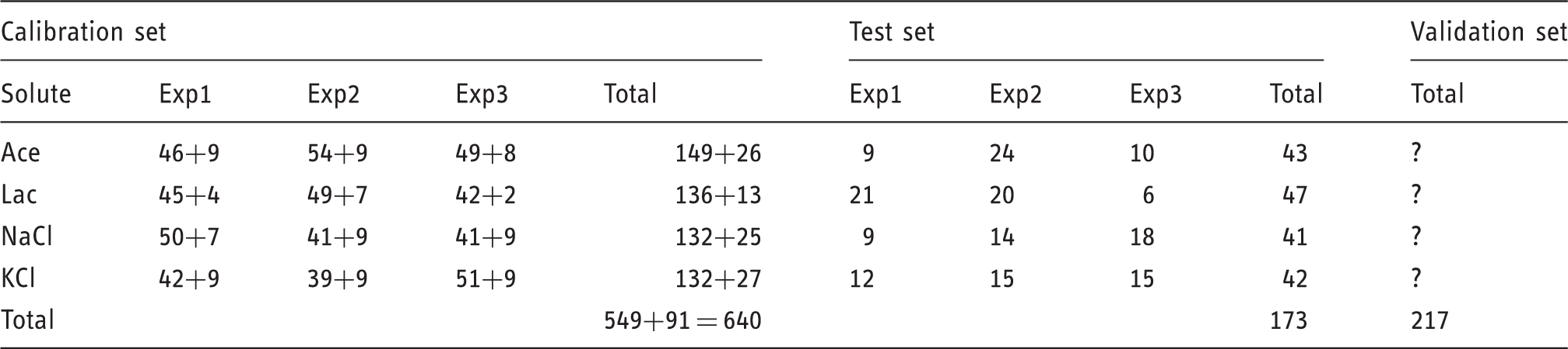
In addition to the data described above, 217 spectra of two unrevealed solution types were also provided for classification purposes without letting the contestant know about their lower concentration (0.1–0.9 mM).

Along with the raw spectra described above, two spectra pre-treatments were provided:

Pure water subtracted⁵ (EA – experimental average): pure water spectra measured in a given experiment were averaged into a single spectrum that was subtracted from solutions that were measured only in that same experiment.

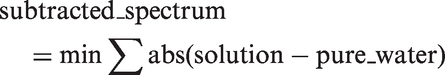
Pure water subtracted⁶ (C – closest pure water): spectra of pure water from all experiments (91 spectra) were subtracted from each solution spectrum (91 × 12 subtracted spectra per concentration level), and the subtracted spectrum with the smallest summed deviation was provided (as the one that most efficiently removed the influence of pure water)

\begin{matrix} subtracted_spectrum \\ = min \sum abs (solution - pure_water) \end{matrix}

The challenge of this shoot-out was to work with water by managing two important sources of spectral variation: concentration and environment-related perturbations. Two ranges of concentrations (low 1–10 mM and high 10–100 mM) were given to illustrate different water–solute interactions that will influence prediction outcomes, while fluctuations in environmental temperature and humidity illustrate environmental variation. The tasks were to:

Predict the concentration of each solute in the validation set

Predict the class of the samples provided in the classification validation dataset in two cases: using only (a) 1–10 mM and (b) the entire (1–100 mM) concentration range.

The next section describes approaches as provided by the four participants.

Participant approaches

Participant 1

For task 1, test partial-least squares (PLS) regressions were conducted using pretreatment combinations of raw, weighted multiplicative scatter correction (MSC) or standard normal variate (SNV) + detrend applied prior to first or second derivative treatments with varying gaps over the entire wavelength range of 1300–1600 nm. This trial and error scheme also included testing various repeatability files⁷ within the Foss WinISI 4 software attempting to minimize temperature and humidity effects. Replicate spectra collected with similar temperature and humidity values were averaged as part of the performance testing. The best performing model for all analytes was observed using the raw calibration set replicates as determined by least root mean square error of cross validation, and thus used for predicting the validation set. The final model spectra for acetic acid utilized first derivative pretreatment with no scatter correction; spectra for the lactose model were corrected only with weighted MSC, whereas NaCl and KCl model spectra underwent SNV and detrend manipulation prior to a PLS regression.

Task 2 was the most challenging, as the classification validation set appeared to contain only samples with low concentration, as predicted by previous models and determined by principal component analysis (PCA) scores. The sample scores for seven PCA latent variables were used as linear discriminant analysis (LDA) predictors using The Unscrambler®. PCA also helped to determine that no KCl samples existed in the validation set, and they were removed from the model. This allowed LDA models to be derived using acetic, lactose, and NaCl spectra only, although the pure water spectra were also included as a separate group during testing. Models were derived with both the full concentration (1–100 mM) and low concentration (1–10 mM) calibration samples. Resulting low concentration classification model statistics were 82% and 92% for the raw and pure water subtracted calibration sets, respectively. Classification between models for the validation set differed greatly, with the most consistent results from the MSC-treated raw spectra, low concentration only model.

Participant 2

The difference between spectra of identical samples measured under varying external factors (humidity, temperature, etc.) can be used as a covariance matrix (also known as interference matrix or clutter). The covariance matrix can then be used to down weight the effect of such interferences via a generalized least-squares based weighting (GLSW) strategy.^8,9 A regularization parameter (alpha) is used in GLSW to adjust the extent of de-weighting (smaller alpha is equivalent to a greater de-weighting). A simplified version of GLSW is called external parameter orthogonalization, which does an orthogonalization (complete subtraction) of some number of significant patterns identified as clutter.¹⁰

To our knowledge, GLSW has not been used in the context of aquaphotomics before. This approach can offer advantages compared to existing methods (water spectrum subtraction or even Extended MSC). In this work, best performance was achieved by applying GLSW on raw spectra (Figure 1). There is an abundance of replicate (water and water/solute) spectra in the challenge data that can serve as an excellent interference matrix for GLSW.

Figure 1.

Applying GLS weighting reveals unique underlying spectral features of different solutes.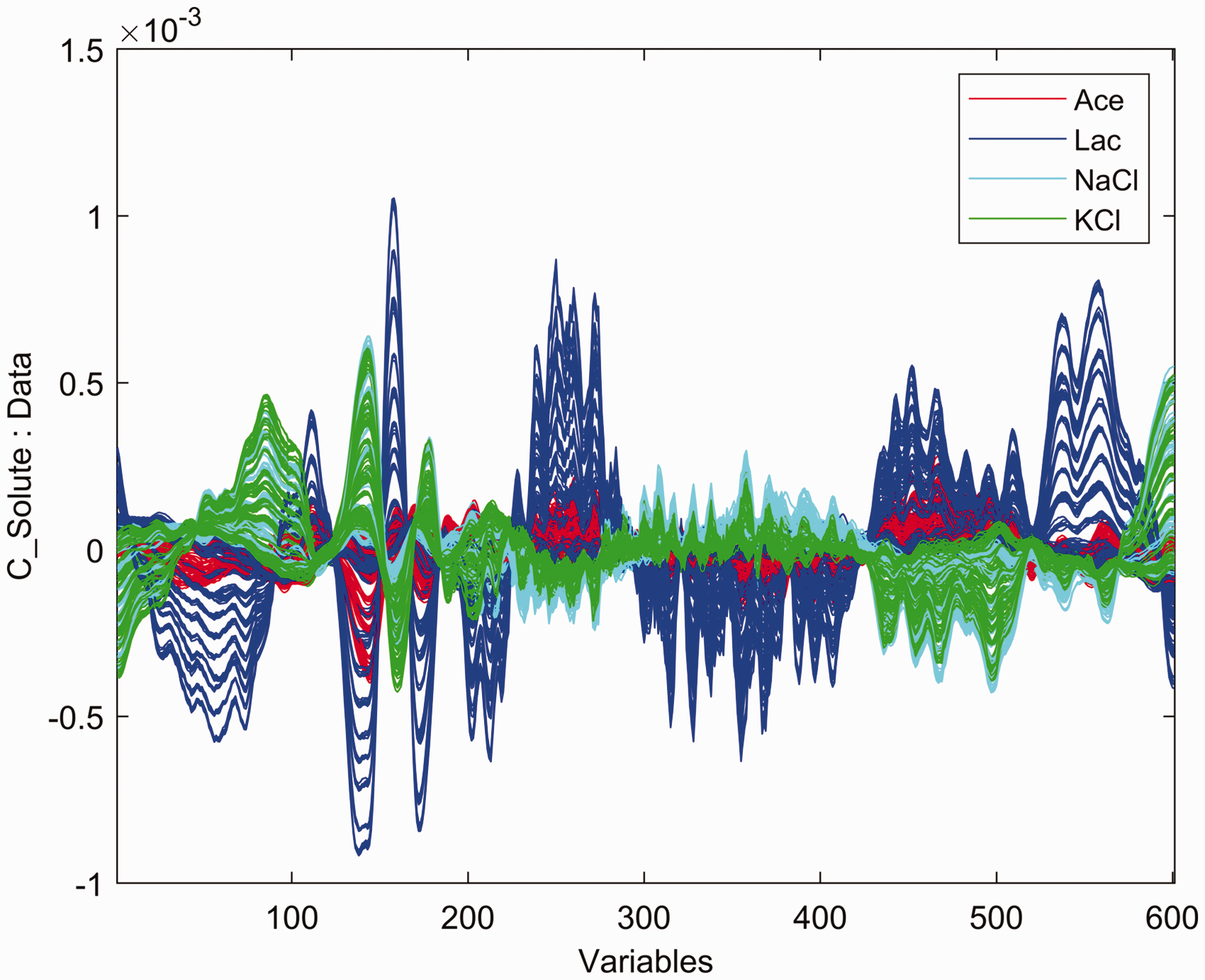

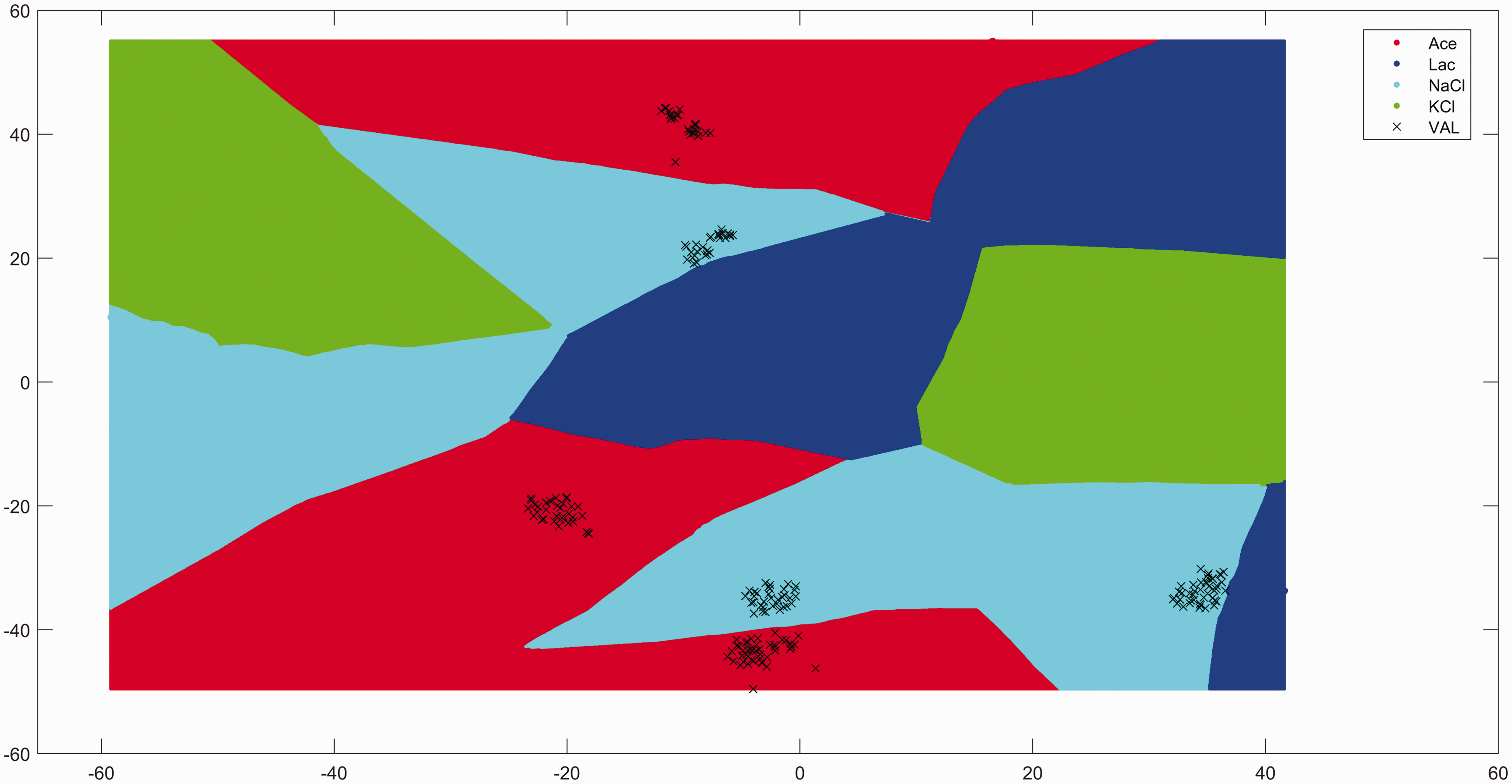
For the classification task, a combination of SNV and GLSW (alpha = 0.0005) was used as pre-processing. This was then followed by a Euclidean k-Nearest Neighbors (KNN) (k = 7) classification step (Figures 2 and 3). For the quantification task, a combination of SNV and GLSW (alpha = 0.001) was used as pre-processing. This was then followed by a variable selection step using recursive PLS¹¹ before applying a locally weighted PLS regression for prediction.

Figure 2.

2D-embedded representation of the original data based on t-SNE approach.¹² The actual KNN predictions are done on the original 601-dimension space.

Figure 3.

Non-linear boundaries are derived from KNN predictions applied on the data grid extracted from Figure 2.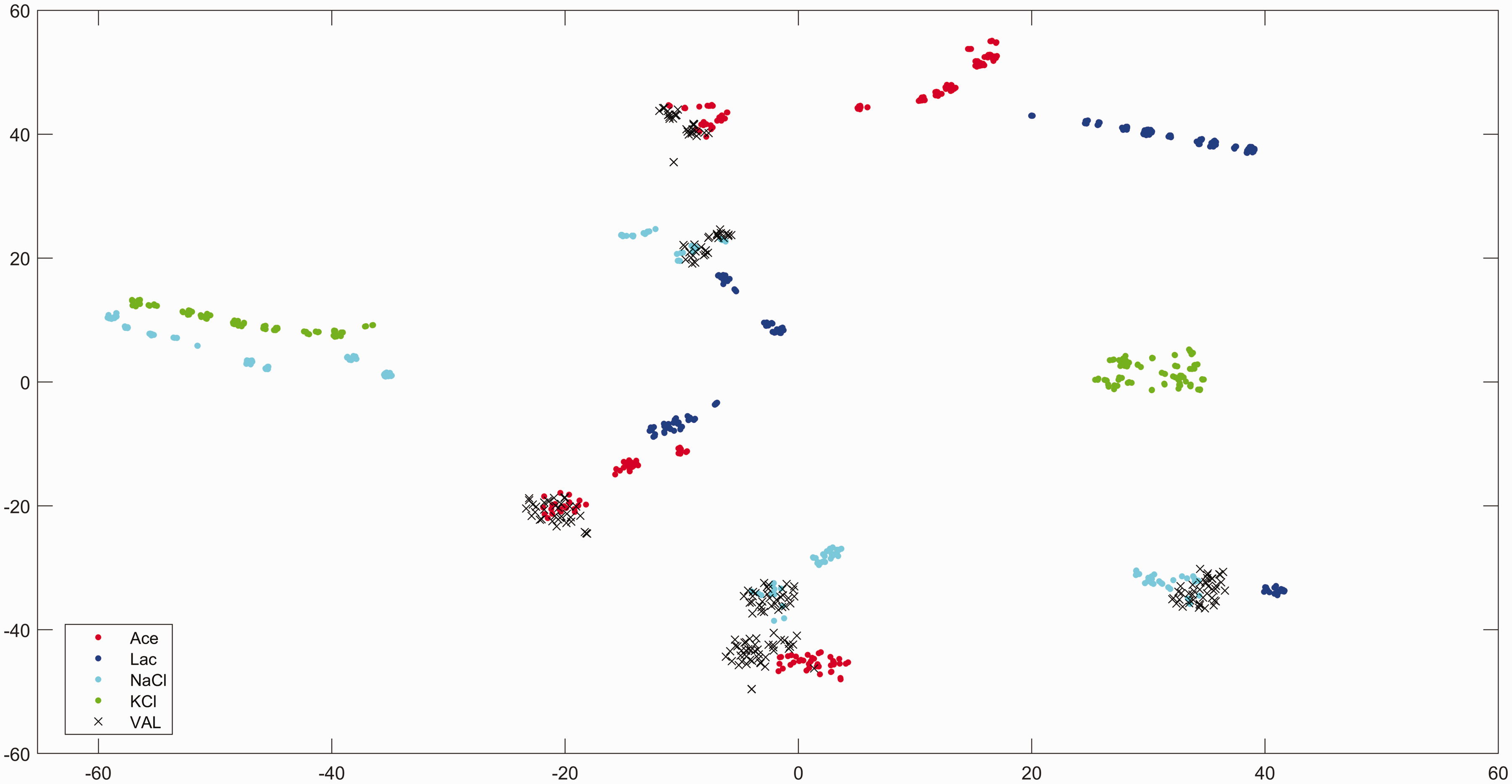

Participant 3

As a relative newcomer to chemometrics, this participant only had access to a specific proprietary PLS software package that was unsuitable to use for these analyses. ‘R’ software is freely available from the CRAN website, and it was selected for EDA and the ‘R’ packages ‘pls’ and ‘mdatools’ were used for PLS and PLS-discriminant analysis/SIMCA, respectively. ‘R’ is a fantastic and very powerful software tool, but it is a scripting language and it is often totally frustrating when some new script will not run until the syntax is totally error free.^13–15 Right at the start of analysis, reading text data into ‘R’ can sometimes be more difficult than expected when for example numeric or integer data are coded as factors or character. All one can say is persist, it gets better.

With the datasets uploaded and available as R objects, plots (see Figure 4 and code below) were obtained using the matplot() function in the ‘R’ base. The plots were visually checked for outliers and some smoothing functions tried but to no real advantage (only added noise).

Figure 4.

Overview/EDA with ‘R’ matrix plot for one of the calibration files from task 1.

Figure 5.

Example of regression coefficient plot output from the PLS ‘R’ package. The model is clearly overfitted when four instead of three PCs are selected.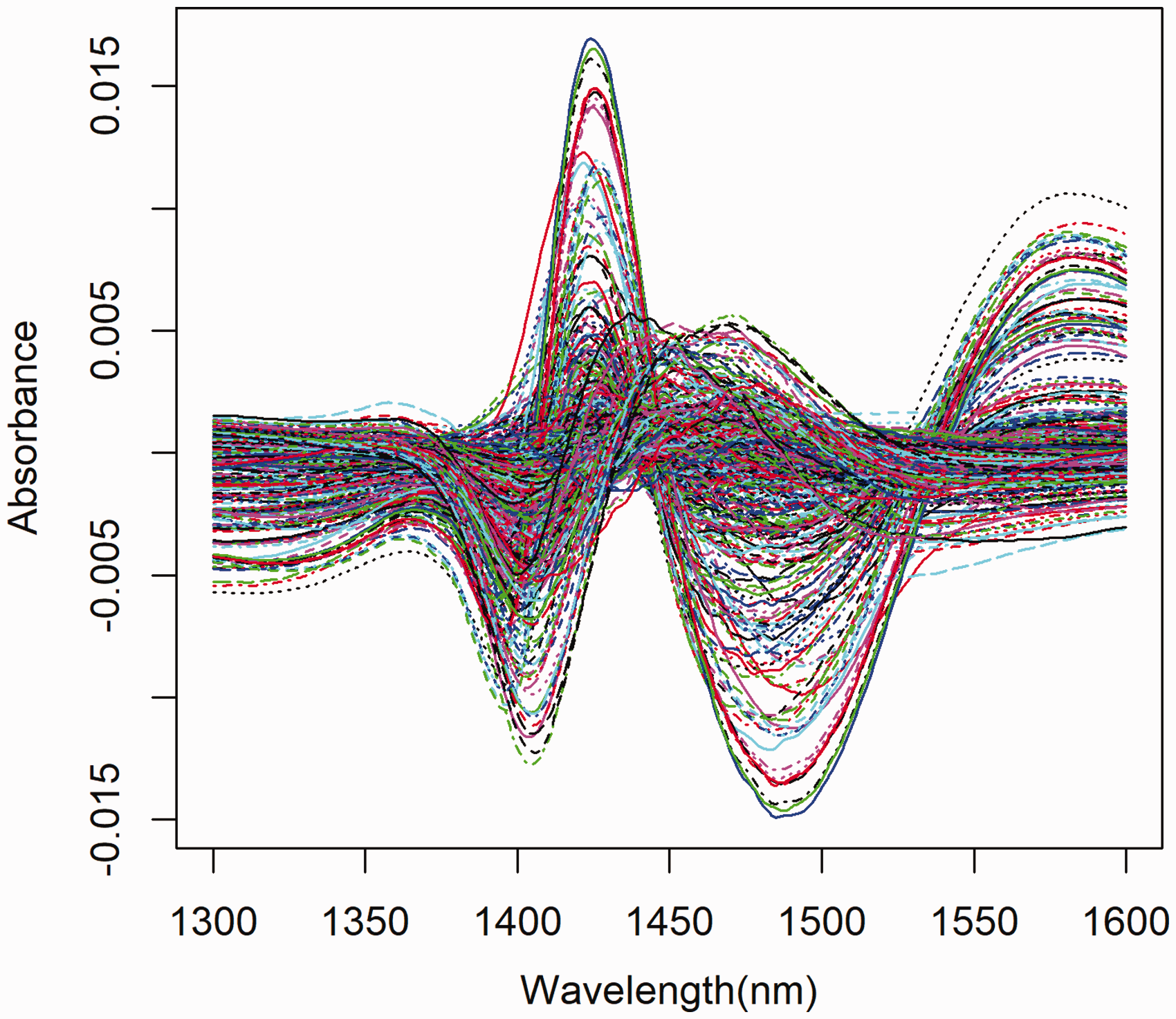

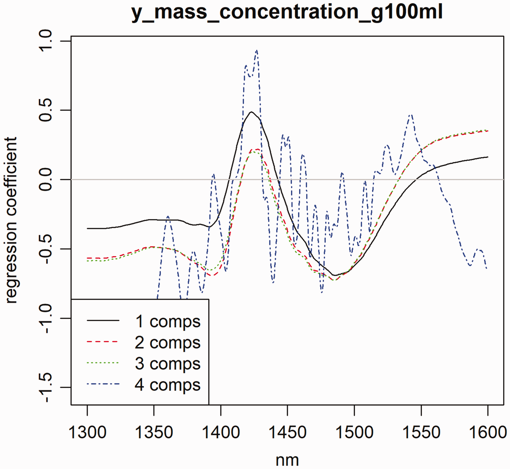
a <- cal_c # data object to plot

x <- which(names(a) %in% c (“ w1300", “ w1600 ”) ) # wavelength range

wl <- names(a[x[1]:x[2]]) # save wavelengths for X-axis

wl <- as.numeric(gsub (‘ w','', wl)) # remove leading w

X <- as.matrix(a[ , x[1]:x[2]]) # convert data to matrix

colnames(X) <- wl # change the matrix column names to wavelength

matplot(as.numeric(colnames(X)), t(X[1:n.r, ] ),

type = “ l", xlab = “ Wavelength(nm)", ylab = “ Absorbance ”) # matrix plot

The training datasets as supplied were used without any pre-treatment to build separate PLS models for each solute. The training models were optimized based on the diagnostic output available from the pls package and by comparison with the test dataset. A plot of the regression coefficients was used to help decide on the number of PCs to try and avoid overfitting (Figure 5). In the code below PLS is called by the plsr() function, data were subset into separate objects by the logical test together with the which() function for each solute in column 2. The NIR wavelength data were first separated and saved as a matrix, protected by the I() function and recombined with the row header information for analysis.

ace_row_nos <- which(cal_c[, 2]== “ Ace ”) # logical test to find only the ace solute rows

NIR <- as.matrix(cal_c[ace_row_nos , x[1]:x[2]]) # subset the ace & wavelength data

cal_c.1 <- cal_c [ c.r.ids, 1:8] # extract the row head info in a new object

cal_c.1$NIR <- I(NIR) # protect NIR matrix and add to the header info

ace <- plsr(y_mass_conc_g100ml ∼ NIR, ncomp = 10, data = cal_c.1, validation = “ LOO ”) # run pls

out.ace$column_x<- predict(ace, ncomp = 3, newdata = val_c) # save predictions vector

write.csv2(out.ace, “best prediction output for acetic acid model.csv ”) # write to export file as csv

This participant struggled with task 2, and used up a lot of time learning the ‘mdatools’ package and writing scripts, rather than really looking at the problem itself and considering the best option for the actual analysis. Exploring the classification problem by first building a PLS model and applying it to the unknown dataset showed clearly that solute concentrations were very low. Without trying to extrapolate the training data in any way to account for the lower concentrations in the unknown data, the approach was to first scale (mean = 0, std = 1) the values and then use the ‘mdatools’ package to run both the simca() and plsda() functions. SIMCA with the low concentration data as a training set gave the best results, but it still failed to classify around 25% of the unknown data. Four separate PCAs were first run for each of the different solutes (each with three PCs) and then each solute model was tested separately against the unknown dataset to be classified. As similar approach was used for partial least-squares discriminant analysis (PLS-DA).

Participant 4

Multivariate models for predicting the solute’s concentration using spectra collected from dispersive instrument were developed. There were four solution systems available varying in the type of solute. In addition, these four systems included samples with high and low solute concentrations. A hierarchal modelling strategy was used to provide a method robust against different solution systems and concentrations. This strategy involved classifying the sample spectra into different groups and then using specifically generated models corresponding to each group.

The first step of the hierarchal strategy was classification. First, all spectra were preprocessed by removing pure water spectral information from each sample spectra using ‘closest pure water’ algorithm. Visual inspection of these preprocessed solution spectra showed distinction between most of the solute systems. However, this distinction was more prominent in higher molar concentration (>1.5 mM), while at lower molar concentration (<1.5 mM), the spectra were similar. Spectrally similar solute groups (especially sodium chloride and potassium chloride), the concentration level, and additional process/environmental factors provided significant challenges in classification of the four solutes (task 2), thus leading to the development of a sequential classification strategy. The first classification performed was to separate the sample into class of high and low molar concentration. This was followed by a second classification step which separated the high molar concentration samples into three groups. Each group corresponded to a specific solute; however, one group was a combination of the solute’s sodium chloride and potassium chloride due to their spectral similarity. All classification analyses were performed using PLS-DA. The classification rate can potentially be further improved by investigating different spectral pretreatments and classification methods.

The second step of the hierarchal strategy was to perform quantitative modelling for solute concentration (task 1). The first step (classification) resolved samples into the following four groups: acetic acid high concentration solution, lactose monohydrate high concentration solution, combination of sodium chloride, and potassium chloride high concentrations solution, and all solute low concentration solution. Four total PLS models were generated corresponding to their respective group. The accuracy of each of the four models was lower than a global PLS model without hierarchal strategy.

Results

Table 2 presents the validation results for each participant. Root mean square errors of prediction are presented along with the classification rate.

Table 2.

Participant performance.

	Participant 1	Participant 2	Participant 3	Participant 4
Regression
Acetic acid	0.0062	0.0051	0.0110	0.0426
Potassium chloride	0.0320	0.0119	1.3014	0.8015
Lactose	0.0055	0.0048	0.2328	0.0322
Sodium chloride	0.0056	0.0057	0.0572	0.0277
Classification, %	43	100	6	23

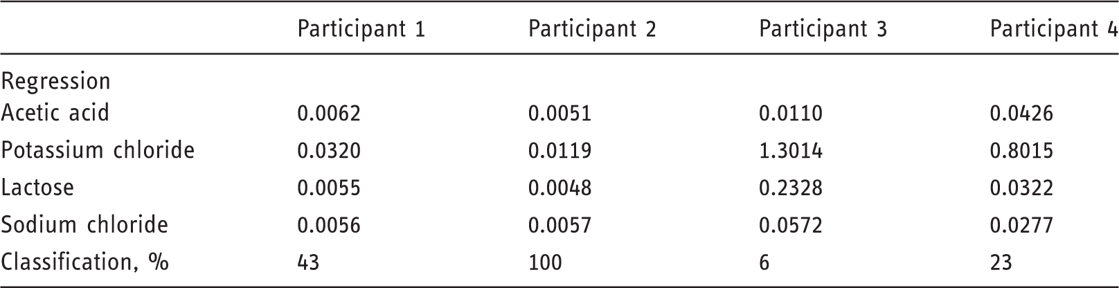
The participants chose quite different approaches to get prediction results that also varied significantly. With the overall best statistics, Participant 2 won the 2018 IDRC Shoot-Out.

The data are available on the IDRC website (http://www.cnirs.org). The authors would like to thank the 2018 IDRC chair Prof. Charles R Hurburgh Jr and the Council for Near-Infrared Spectroscopy for providing funding for the shoot-out and support for the conference. The next conference will take place in the summer 2020.

Footnotes

Declaration of conflicting interests

The author(s) declared no potential conflicts of interest with respect to the research, authorship, and/or publication of this article.

Funding

The author(s) received no financial support for the research, authorship, and/or publication of this article.

References

Igne

Dardenne

Honigs

et al.

The 2010 IDRC software shoot-out at a glance. NIRNews 2010; 21: 14–16.

Igne

Berzaghi

et al.

Summary of the 2012 IDRC software shoot-out. NIRNews 2012; 23: 13–15.

Igne

Bogomolov

et al.

Summary of the 2014 IDRC software shoot-out. NIRNews 2014; 26: 8–11.

Igne

Alam

et al.

Summary of the 2016 IDRC software shoot-out. NIRNews 2017; 28: 16–22.

Kovacs

Bazar

Oshima

et al.

Water spectral pattern as holistic marker for water quality monitoring. Talanta 2016; 147: 598–608.

Kojić

Tsenkova

Yasui

. Improving accuracy and reproducibility of vibrational spectra for diluted solutions. Anal Chim Acta 2017; 955: 86–97.

Westerhaus

Improving repeatability of NIR calibrations across instruments. In: Biston

Bartiaux-Thill

(eds). Proceeding third international conference near infrared spectroscopy, Gembloux, Belgium: Agricultural Research Centre Publishing, 1990, pp. 671–674.

Martens

Høy

Wise

et al.

Pre-whitening of data by covariance-weighted pre-processing. J Chemometr 2003; 17: 153–165.

Eigenvector research. Glsw, http://wiki.eigenvector.com/index.php?title=Glsw (2015, accessed 14 November 2018).

10.

Roger

J-M

Fabien

Véronique

B-M

. EPO–PLS external parameter orthogonalisation of PLS application to temperature-independent measurement of sugar content of intact fruits. Chemometr Intell Lab Syst 2003; 66: 191–204.

11.

Rinnan

et al.

Recursive weighted partial least squares (rPLS): an efficient variable selection method using PLS. J Chemometr 2014; 28: 439–447.

12.

The Mathworks. T-SNE, https://uk.mathworks.com/help/stats/t-sne.html (2018, accessed 10 November 2018).

13.

R Core Team. R: A language and environment for statistical computing, Vienna, Austria: R Foundation for Statistical Computing, 2017.

14.

Mevik B-H, Wehrens R and Liland KH. pls: partial least squares and principal component regression. R package version 2.7-0. https://cran.r-project.org/web/packages/pls/index.html (2018, accessed 10 November 2018).

15.

Kucheryavskiy S. mdatools: multivariate data analysis for chemometrics. R package version 0.9.1, https://cran.r-project.org/web/packages/mdatools/index.html (2018, accessed 10 November 2018).