A comparison of methods for sample size estimation for non-inferiority studies with binary outcomes

Abstract

Non-inferiority trials are motivated in the context of clinical research where a proven active treatment exists and placebo-controlled trials are no longer acceptable for ethical reasons. Instead, active-controlled trials are conducted where a treatment is compared to an established treatment with the objective of demonstrating that it is non-inferior to this treatment. We review and compare the methodologies for calculating sample sizes and suggest appropriate methods to use. We demonstrate how the simplest method of using the anticipated response is predominantly consistent with simulations. In the context of trials with binary outcomes with expected high proportions of positive responses, we show how the sample size is quite sensitive to assumptions about the control response. We recommend when designing such a study that sensitivity analyses be performed with respect to the underlying assumptions and that the Bayesian methods described in this article be adopted to assess sample size.

Keywords

sample size power non-inferiority parallel group clinical trials sensitivity analysis Bayesian methods

1 Introduction

Studies with non-inferiority as the primary objective are becoming an increasingly common type of trial in clinical research. This is because for trials where a proven active treatment exists, due to ethical pressures, placebo-controlled trials are increasingly discouraged. Non-inferiority trials are also becoming more common in other forms of health technology assessment such as role replacement studies. In both instances, the objective is to determine whether the investigative intervention is no worse or non-inferior clinically to the standard treatment. For example in a drug trial, the objective would be to assess whether the new drug is non-inferior to the standard drug, or in the context of a role replacement, the objective would be to assess, say, whether a nurse is non-inferior compared to a doctor for a given role.

In non-inferiority trials, the objective is to assess whether the investigative intervention is no worse than the standard not whether they are the same or equivalent. This assessment is made with reference to a non-inferiority limit or margin, d, where non-inferiority of a new treatment is usually determined by comparing the worst tail of 95% confidence interval with the non-inferiority margin to rule out the inferiority of a new treatment.

The evaluation of d requires consideration of several aspects including the minimal clinically important difference and the known data on the active compactor. Generally, it is defined as the largest difference that is clinically acceptable such that a larger difference than this would matter in clinical practice.¹ In addition it cannot be ‘greater than the smallest effect size that the active (control) drug would be reliably expected to have compared with placebo in the setting of the planned trial,’² a statistical assessment. There are European guidelines on the topic.³ In spite of such definitions and guidance, the choice of d may remain controversial in a particular context.

If upon completing the study, there is evidence to suggest that a new intervention is superior to the standard, for example, that a nurse is superior to a doctor for a given role, then this conclusion would be acceptable provided such a possibility has been referred to as an objective in the protocol a priori. Non-inferiority studies are distinct from equivalence studies, where the objective in the latter is to demonstrate that neither intervention is inferior to the other.^4,5 In fact the assessment of both non-inferiority and superiority can be assessed in a hierarchical testing framework.^4,6 Trials designed to assess of both superiority and non-inferiority objectives are described as ‘as good as or better’ trials.^4,6 For such studies, there are regulatory guidelines.¹ This article will concentrate on the design of non-inferiority studies only.

The context for this article is that we wish to be able to design trials for non-inferiority parallel group studies where the primary outcome is binary, but we anticipate a high positive response rate on both the investigative and control arms (≥70%). The primary outcome is the difference in the absolute risk response with its corresponding two-sided 95% confidence interval. Non-inferiority is to be assessed from the lower (or upper) bound (depending on the direction of interest) of the two-sided 95% confidence interval, which is consistent with a one-sided test at the 2.5% level of significance.

An important consideration in the designing of any trial is the sample size estimation. An issue with respect to the studies being considered in this article is that the confidence intervals in each individual study could be calculated using one of four methods as follows: normal approximation, normal approximation with continuity correction, Wilson’s score and Wilson’s continuity corrected score. The choice of one of these four different approaches may influence how the sample size may be calculated. In addition to four different approaches to calculating a confidence interval there are a number of ways to calculate the sample size (three will be described), which makes for 12 different design and analysis combinations.

In calculating a sample size, we therefore need to consider the context of the objective of the trial (non-inferiority), design (parallel group), the primary outcome (binary), method of confidence interval calculation and the response rates anticipated (here assumed ≥70%). We make this assessment through a simulation.

The concentration in the article is the situation where the trial is to be summarised as a difference in the anticipated absolute risks. However, the same principles discussed in the article also hold, however, if we are to use odds ratios, as the variance for the odds ratio is (approximately) equal to the reciprocal to the variance of the absolute risk difference such that (OR) ∝ 1/var(p_A – p_B)⁷

The calculation itself would be critically dependent on the control response rate that would usually be estimated, maybe imprecisely, from a previously conducted trial. The sample size calculation could therefore be sensitive to the assumptions about the estimated control response. We will describe how to investigate this sensitivity and to account for the imprecision in the estimated control response in sample size calculations.

2 Setting the null and alternative hypotheses

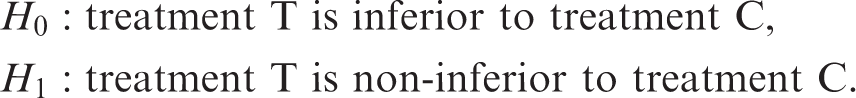
Let π_C and π_T denote the true but unknown (population) proportions of positive responders to treatment on drugs C and T, respectively (note we adhere to the convention of using Greek letters to denote (unknown) population parameters). The context here is that C is the standard or control treatment, T is the test treatment and the direction of interest is positive, that is, larger population parameters are better. For non-inferiority trials, the appropriate null (H₀) and alternative (H₁) hypotheses are as follows:

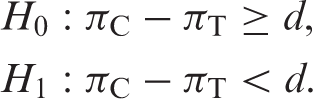
Or, alternatively as the following:

Here d is the non-inferiority margin.^1,8,9 For the a priori quantification of d, there are general European guidelines.³ In the context of the problem here, d > 0 would equate to a test of non-inferiority, while a d ≤ 0 would equate to a test of superiority.

The standard approach is to test the null hypothesis using a one-sided test. For one-sided tests, the convention is to set the significance level at half of that of a two-sided test, that is, a 2.5% level of significance.¹⁰ Operationally, however, non-inferiority is investigated through constructing a central 95% confidence interval and declaring non-inferiority if the appropriate (lower or upper) bound excludes the limit d.¹ This is the same as doing a one-sided test at the 2.5% level of significance or calculating a one-tailed 97.5% confidence interval.

3 Calculation of confidence intervals for the difference in absolute response

Since π_C and π_T are unknown, we need to undertake a trial to make inference about them. We will denote as p_C and p_T as point estimates, respectively, for π_C and π_T. Here, we are primarily interested in evaluating the difference in response via the point estimate p_C − p_T of the difference π_C − π_T. In conjunction with these point estimates, confidence intervals are calculated to provide a range of plausible values for π_C − π_T.

Four methods of confidence interval estimation are given Table 1. The form of confidence interval estimation is particularly important for non-inferiority studies as it is from the confidence intervals that we tend to conclude (or not) non-inferiority.

Table 1.

Four different approaches for calculating confidence intervals for a binary response

	Without continuity correction	With continuity correction
Normal approximation	(1) where (2) and Z_{1 – α/2} is the (1 – α/2)-th percentile of the standard normal distribution. This method is referred to as the Wald method.¹¹	An addition to the right-hand side of Equation (2) of (1/n_C+1/n_T)/2 is added^11,12 such that: where (3)
Wilson’s score	The lower bound for confidence inter val (L) for the difference in proportions p_C – p_T is defined as: ¹¹ (4) while the upper bound is defined as: (5) Here, l_C and u_C are the lower and upper bounds for p_C, and l_T and u_T are the lower and upper bounds for p_T. These are obtained from the following for p_C and p_T:^11,13 (6) (7)	Derived as per Equations (4) and (5) but with l_C, u_C, l_T and u_T (the lower and upper bounds for p_A and p_B, respectively) obtained from the following for p_C and p_T: (8) (9)

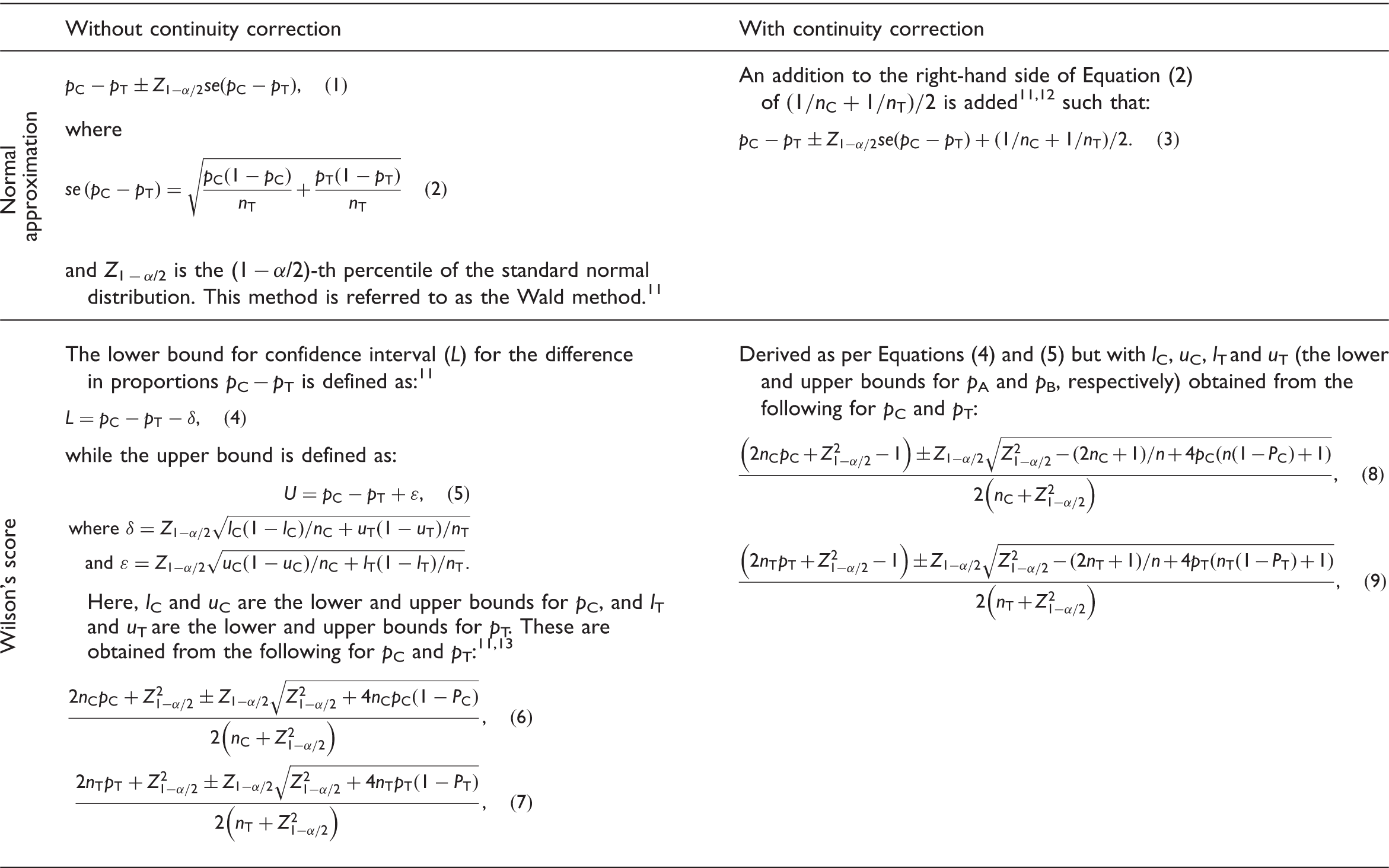
We only describe four methods here, which although not comprehensive of all methods (for alternative methods, see Newcombe¹¹), they represent the methods considered in the individual trials we are planning. In the main, we use normal approximation methods for calculating confidence intervals, but for trials where we anticipate a high response rate (>90%), we consider ‘Wilson’s score’ method, which has been shown to have superior nominal coverage compared to normal approximation approaches.¹¹

4 Sample size estimation: population responses assumed known

Unlike the case of normally distributed data where the variance is the same irrespective of which hypothesis is true, the variance of a binary variable depends on the outcome probabilities, which is an added complication in the assessment of sample size. 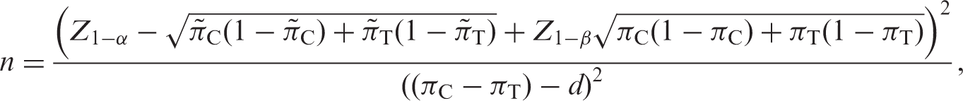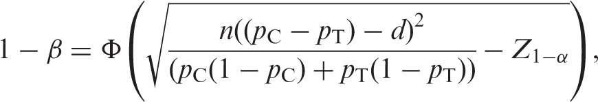There is a further issue in calculating the sample size per group, in that under both the null and alternative, there is often a non-zero difference between treatments.¹⁴ Generally, for a non-inferiority study, the sample size for a one-sided test at a significance level α can be regarded as based on the formula:

(10)

where n is the sample size per group, Z_{1 −} _α is the 100(1 − α)-th percentile of the standard normal distribution and the variances in the square root terms refer to the variances about the difference in the population responses under the null and alternative hypotheses. Now Equation (10) can, in turn, be thought of in terms of:

(11)

where

\tilde{π}

and π_C are estimates of the responses on each treatment under the null hypothesis used to estimate the variance about the difference under this hypothesis, that is:

(12)

Here n is the sample size on both T and C, respectively. Now, for non-inferiority trials, we often have that π_T ≠ π_C under both the null and alternative hypotheses, that is, the two treatments do not have an equal response. Note that the hypothesis influences the variance under this hypothesis because the estimates of π_T and π_C affect the estimate of the variance. Table 2 gives the definition of three methods for sample size calculation. Note in this article, we will concentrate on the special case of n = n_C = n_T.

Table 2.

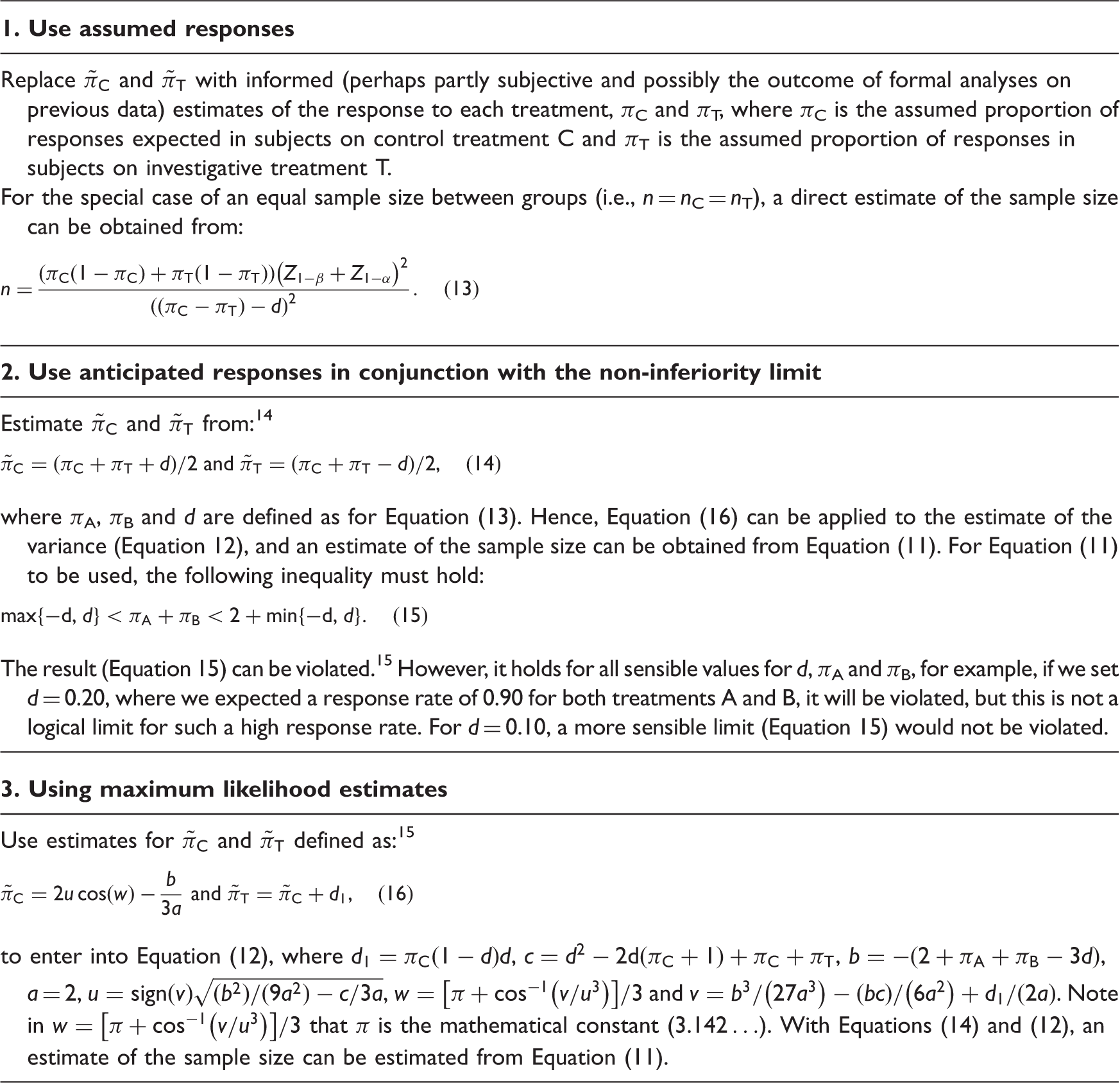
Three different methods for estimating the sample size for a non-inferiority trial with a binary response

1. Use assumed responses

Replace

{\tilde{π}}_{C}

and

{\tilde{π}}_{T}

with informed (perhaps partly subjective and possibly the outcome of formal analyses on previous data) estimates of the response to each treatment, π_C and π_T, where π_C is the assumed proportion of responses expected in subjects on control treatment C and π_T is the assumed proportion of responses in subjects on investigative treatment T.

For the special case of an equal sample size between groups (i.e., n = n_C = n_T), a direct estimate of the sample size can be obtained from: (13)

2. Use anticipated responses in conjunction with the non-inferiority limit

Estimate

{\tilde{π}}_{C}

and

{\tilde{π}}_{T}

from:¹⁴

(14)

where π_A, π_B and d are defined as for Equation (13). Hence, Equation (16) can be applied to the estimate of the variance (Equation 12), and an estimate of the sample size can be obtained from Equation (11). For Equation (11) to be used, the following inequality must hold:

(15)

The result (Equation 15) can be violated.¹⁵ However, it holds for all sensible values for d, π_A and π_B, for example, if we set d = 0.20, where we expected a response rate of 0.90 for both treatments A and B, it will be violated, but this is not a logical limit for such a high response rate. For d = 0.10, a more sensible limit (Equation 15) would not be violated.

3. Using maximum likelihood estimates

Use estimates for

{\tilde{π}}_{C}

and

{\tilde{π}}_{T}

defined as:¹⁵

(16)

to enter into Equation (12), where d₁=π_C(1 − d)d, c=d² − 2d(π_C+1)+πC+π_T, b=−(2+π_A+π_B − 3), a=2,

u = sign (v) \sqrt{(b^{2}) / (9 a^{2}) - c / 3 a}

, w=[π+cos⁻¹ (v/u³)]/3 and v=b³ (27a³) − (bc)/(6a²)+d¹/(2a). Note in w=[π+cos⁻¹ (v/u³)]that π is the mathematical constant (3.142 …). With Equations (14) and (12), an estimate of the sample size can be estimated from Equation (11).

4.1 Comparison of the three methods of sample size estimation

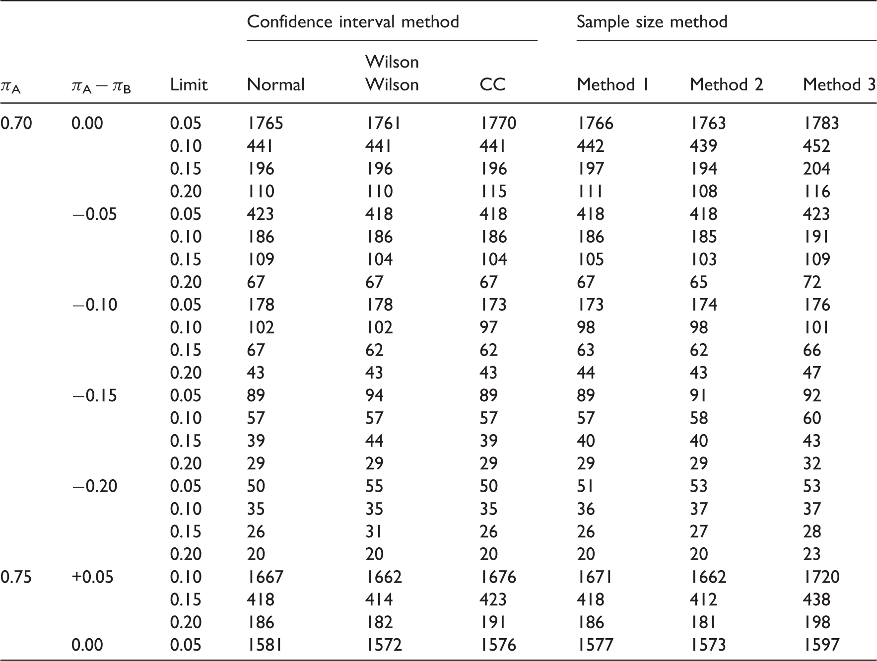
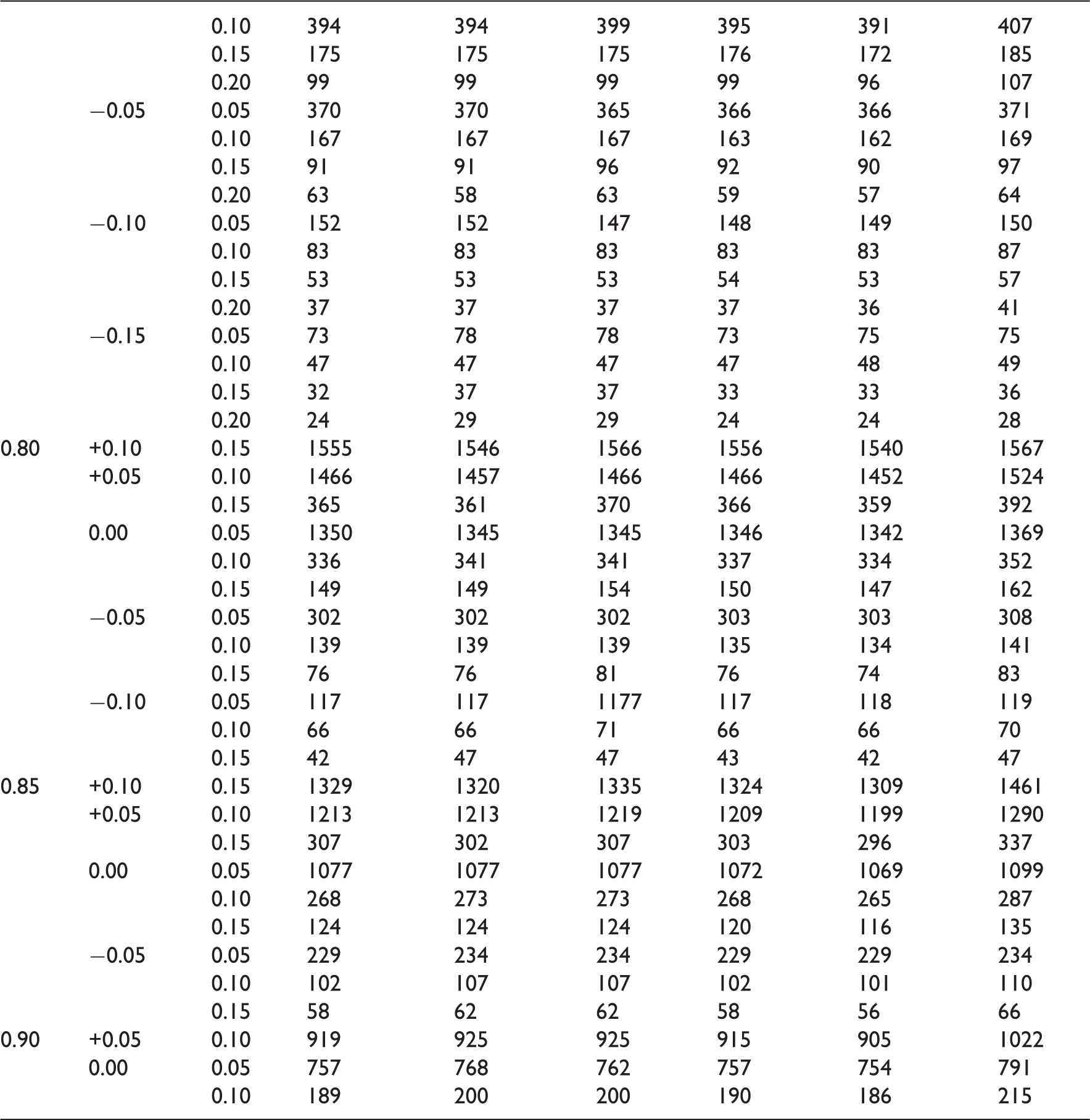
As evidenced by their descriptions, the three methods for estimating the variance under the null hypothesis are markedly different. As a result, they give different estimates for the sample size. To compare the three methods of sample size estimation, a simulation was undertaken. The simulation was undertaken for different responses to treatment (π_A and π_B) between 0.70 and 0.90 and non-inferiority limits, d, between 0.05 and 0.20. For each d, π_A and π_B, the sample size was iterated until the required power was reached. A total of 100 000 simulations were undertaken to estimate the power for each n, d, π_A and π_B. The simulation was undertaken in SAS.¹⁶

The simulation was repeated for the four different methods of calculating confidence intervals described in Table 1. The simulations were stopped when the requisite proportion of simulations (90%) had an upper tail of a 95% confidence interval less than d. The normal approximation with continuity correction gave substantially larger estimates of the sample size compared to the other three and are not included here.

The detailed results of the simulation are given in Table A1 in the Appendix. Table 3 gives summary statistics for the ratio of the estimated sample size over that from the simulations.

Table 3.

A simulation comparison of three different methods of sample size estimation for a non-inferiority study: Method 1 (using assumed responses), Method 2 (using anticipated responses in conjunction with the non-inferiority limit) and Method 3 (using maximum likelihood estimates)

CI calculation	Statistic	Method of sample size calculation
CI calculation	Statistic	Method 1	Method 2	Method 3
Normal approximation	Minimum	0.93	0.90	0.97
	Quartile 1	0.99	0.97	1.02
	Median	1.00	0.99	1.05
	Quartile 3	1.00	1.00	1.08
	Maximum	1.01	1.05	1.16
Wilson	Minimum	0.82	0.81	0.90
	Quartile 1	0.97	0.97	1.01
	Median	1.00	0.98	1.04
	Quartile 3	1.00	0.99	1.07
	Maximum	1.02	1.03	1.11
Wilson with continuity correction	Minimum	0.82	0.81	0.94
	Quartile 1	0.97	0.95	1.02
	Median	0.99	0.98	1.04
	Quartile 3	1.00	1.00	1.06
	Maximum	1.01	1.05	1.11

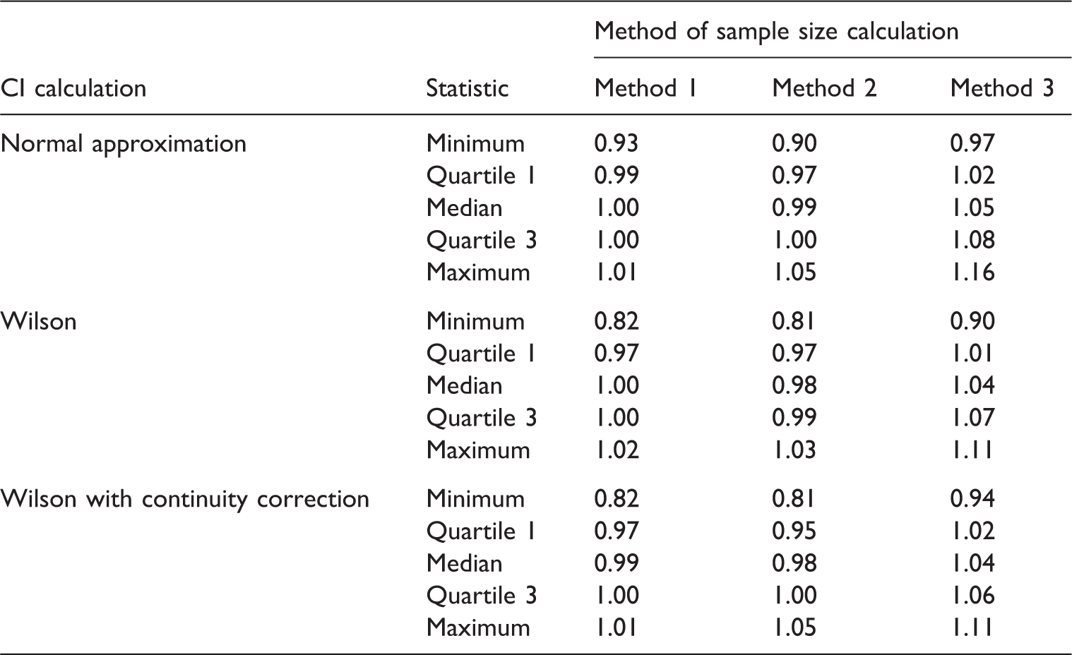
Within the parameters of the simulation, it seems that which sample size method to use depends on preference towards various aspects of the results. Method 1 gives the closest estimates compared to simulations, whereas Method 3 it seems best guarantees to have the nominal level of power as it would seem to over estimate the sample size compared to simulations. With Method 1 there could be instances, from the simulations, when the sample size is under estimated, meaning the trial may have less power than the nominal level.

The limitation of the simulation was that we used approximations to the normal distribution for both the confidence interval and sample size estimation. This would seem reasonable given the range of anticipated responses we simulated within. However, these normal approximations may not hold if, for example, we had very high anticipated response (>90%) and so alternative methods may need to be considered.¹⁷

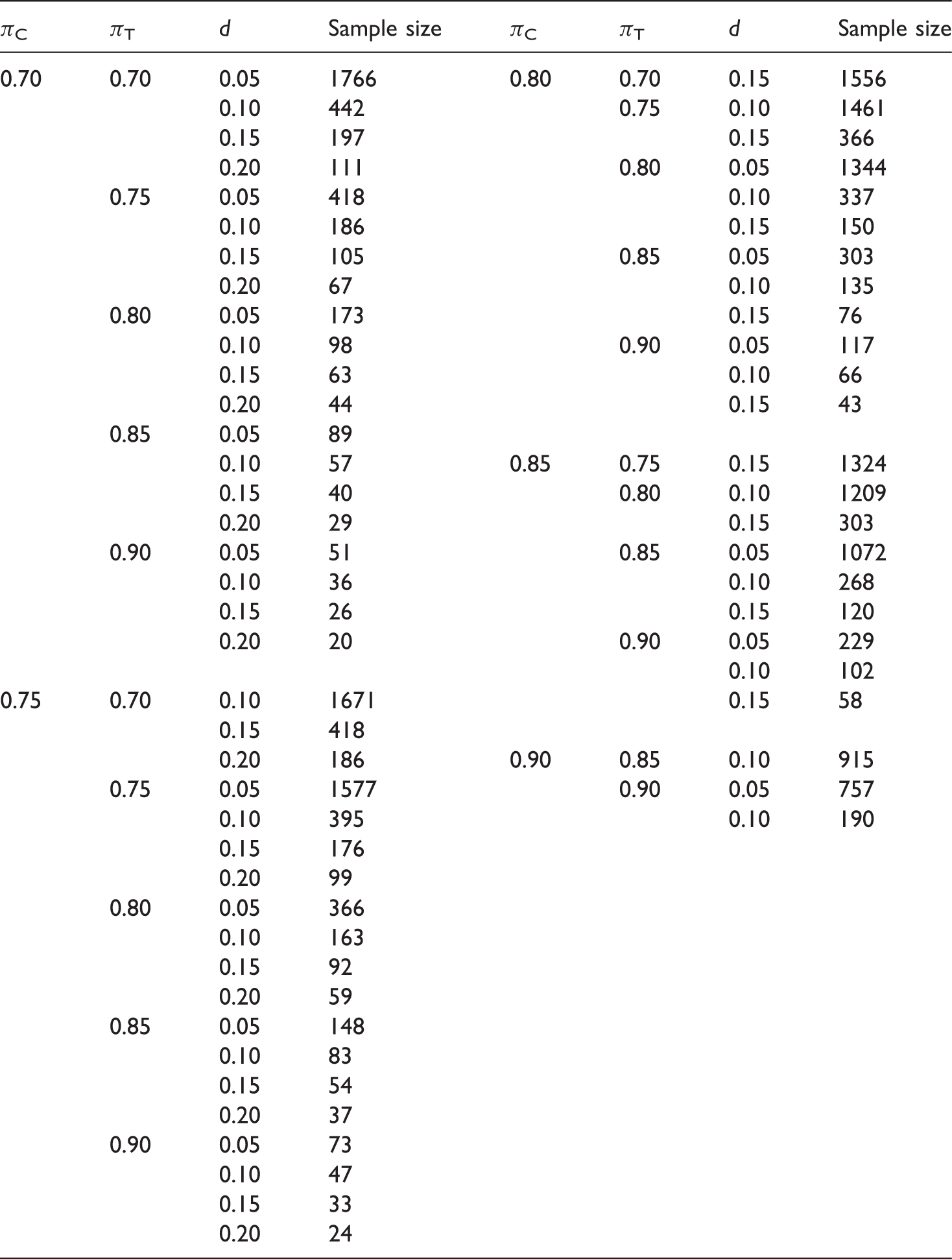
From this point in the article, we will concentrate on using Method 1 for sample size calculations. Table 4 gives the sample sizes for the different response rates for the investigative and control treatment from Equation (13).

Table 4.

Sample sizes for a non-inferiority study estimated for 90% power and a Type I error rate of 2.5% for various anticipated responses and non-inferiority limits δ

π _C	π _T	d	Sample size	π _C	π _T	d	Sample size
0.70	0.70	0.05	1766	0.80	0.70	0.15	1556
		0.10	442		0.75	0.10	1461
		0.15	197			0.15	366
		0.20	111		0.80	0.05	1344
	0.75	0.05	418			0.10	337
		0.10	186			0.15	150
		0.15	105		0.85	0.05	303
		0.20	67			0.10	135
	0.80	0.05	173			0.15	76
		0.10	98		0.90	0.05	117
		0.15	63			0.10	66
		0.20	44			0.15	43
	0.85	0.05	89
		0.10	57	0.85	0.75	0.15	1324
		0.15	40		0.80	0.10	1209
		0.20	29			0.15	303
	0.90	0.05	51		0.85	0.05	1072
		0.10	36			0.10	268
		0.15	26			0.15	120
		0.20	20		0.90	0.05	229
						0.10	102
0.75	0.70	0.10	1671			0.15	58
		0.15	418
		0.20	186	0.90	0.85	0.10	915
	0.75	0.05	1577		0.90	0.05	757
		0.10	395			0.10	190
		0.15	176
		0.20	99
	0.80	0.05	366
		0.10	163
		0.15	92
		0.20	59
	0.85	0.05	148
		0.10	83
		0.15	54
		0.20	37
	0.90	0.05	73
		0.10	47
		0.15	33
		0.20	24

4.2 Worked Example 1 – standard sample size calculation

An investigator wishes to design a trial where the anticipated response rate on the active control is 85%. The investigator also expects an 85% response rate on the investigative therapy. The non-inferiority limit will be set at 15%. The power for the study is to be set at 90%, and it is to have a one-sided Type I error of 2.5%. From Table A1 with this non-inferiority limit, Method 1 estimates the sample size to be 120.

5 Sample size estimation: population responses assumed unknown

The sample size calculations described so far in the article have assumed the control and investigative responses are known. In practice, it would often be the control response that would assumed to be known, with an estimate of the likely investigate response made from this. The estimate of the control response would likely come from a previously conducted trial, which included the control therapy as a treatment arm. The sample size calculation could therefore be sensitive to the assumptions about the estimated control response. We will now describe how to investigate this sensitivity and to account for the imprecision in the estimated control response in sample size calculations.

5.1 Sensitivity analysis about the estimates of the population effects used in the sample size calculations

With a binary response, a main factor to which a non-inferiority study is sensitive is the anticipated response rate on control, which is usually an estimate from a previous study, p_C. This is because this response rate in turn feeds into the estimate of variance used in the calculations and can influence the non-inferiority margin.¹⁸

The sensitivity of a non-inferiority study design to the estimated control response rate could be investigated through construction of a 95% confidence interval around this response. The power could then be assessed at the two tails of the confidence interval for the control response rate from:

(17)

where n is the estimated sample size from (13), and p_C is the plausibly high or low (from the 95% confidence interval) response rate for the control. Consequently, p_T is assumed to be the investigative response (used in the original calculation) and d the non-inferiority margin.

5.1.1 Worked example 2 – investigating sensitivity

Suppose the worked example given earlier to the control response rate was assessed from a previous study in 100 patients, it was assumed that the investigative response rate is correct at 85% with a confidence interval that indicates a plausible range for the control response to be between 78% and 92%.

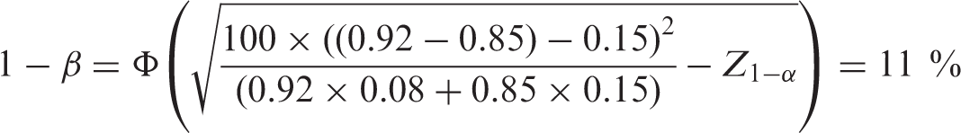
From (17) we could investigate the power of the study supposing a plausibly high value for the control response was nearer to the true response, but the investigative response was 85%, that is,

An equivalent calculation could be done for a plausibly low control response. Table 5 gives a breakdown of the sensitivity of the study design for the estimation of the control response rate. For this example, it is the upper point of the confidence interval to which the study is sensitive.

Table 5.

Sensitivity analysis for non-inferiority worked example

	Observed	95% confidence interval
	Observed	Lower	Upper
Control response	0.85	0.78	0.92
Non-inferiority margin	0.15	0.15	0.15
Investigative response	0.90	0.85	0.85
Power	90%	>90%	11%

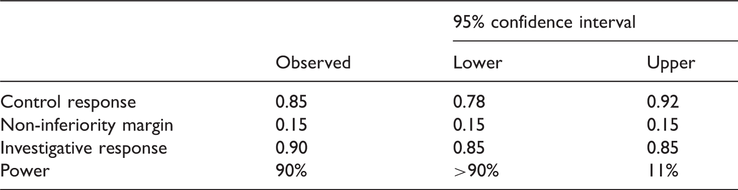
For this worked example, therefore, we have designed a study with 90% power based on a previously observed control response rate of 85%. If the true control response rate is nearer to 78% (which is plausible based on the confidence interval), then we would have greater power than the nominal power set a priori. However, if the control response was truly 92%, then our power could be as low as 11%.

Note in this example, when assessing the sensitivity, it was assumed that if we observed a lower or higher than expected control response rate, then the original non-inferiority would still be used. However, if a higher than expected control response rate was observed, this may not be appropriate.

5.2 π’s or p’s

Note that in this article, we adopt the fairly standard convention, that is, the Greek letters are used for unknown parameter values and Latin letters for their estimates.

In the context of designing clinical trials with a binary response, a thing to be noted in this article is the flip flopping between π’s or p’s. To a degree, this is unavoidable, although admittedly a little confusing. For inference, π’s are taken as the known population estimates for the absolute risks, whereas p’s are taken as sample estimates (from a trial) of π. Hence, in the discussion of confidence intervals, we will quote p’s in the results as we are talking about sample estimates.

For sample size calculations, we mainly assume that absolute response is known for the sample size calculation and so we quote π’s. This is contradicted of course by our need to do a trial to try and quantify them. It is further contradicted by the fact that we take π’s often as estimates (p’s) from a retrospective study.

It is a Gordian knot. Making assumptions about the populations is one that we need to make in all sample size calculations and one to which sample size calculations are very sensitive, which we have discussed throughout the article.

5.3 Calculations taking account of the imprecision of the estimates of the population effects used in the sample size calculations

If the sample size calculations are sensitive to assumptions about the control response rate, p_C, then it may be worth considering sample size calculations that account for the imprecision in p_C. This could be done as follows.

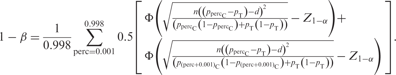
Assume in this instance that the control response rate, p_C, is estimated from a previous study. Using an appropriate confidence interval methodology, an estimate of the first, second, third percentile, say, of p_C can be made based on the previously observed p_C. Here, these percentiles will be estimated using a normal approximation. Hence, percentiles for the control response 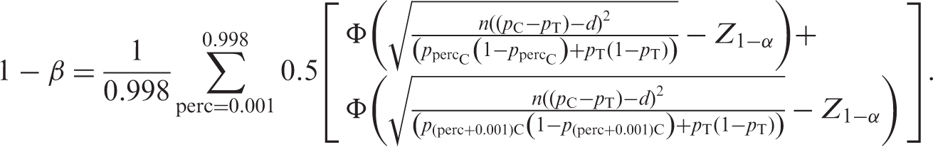$p_{{perc}_{C}}$ could be estimated equating to the 0.1% point for p_C, the 0.2% point and so on. Assuming the difference between the two treatments, p_C − p_T as well as the investigative response, p_T, are fixed then an estimate of the power for a given n and imprecision about p_C can be made from:

(18)

Consequently, the sample size can be estimated through iteration, that is, for each n, we can estimate the power of the study and we iterate on n until the requisite power is reached.

5.3.1 Worked example 3 – accounting for the imprecision in estimate of the control response

Suppose that the investigator wishes to re-interrogate the calculation, from Worked Example 1, to allow for the fact that the control response rate was estimated from 100 patients. From (18), the sample is estimated to be 122 patients per arm. This is 2 greater than the calculation done earlier.

5.4 Calculations taking account of the imprecision of the estimates used in the calculation of sample sizes – Bayesian methods

So far, we have described conventional sample size calculations and discussed how these may be sensitive to the assumptions about the control response rate, p_C.

There may be situations where there is a degree of disbelief in the control response rate. For example, the study upon which it is estimated may have been undertaken in a different trial population or some time in the past such that there now may be a belief that the response in the current study may truly be higher. As we have previously demonstrated a study may be quite sensitive to the assumptions about the control response.

One solution could be to ignore the previously observed trial data and simply use what is believed to be the control response in the sample size calculations using (13). If there is a particularly strong justification for this then this may be appropriate. However, we could be discarding valid empirical information. What we wish therefore to do is to combine the observed data with what we believe to estimate likely responses for the control responses. A Bayesian approach that formally combines the two aspects seems a logical solution.

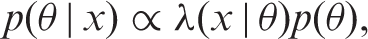
For the given sample size, what needs to be determined is the probability of observing a given control response, $p_{C_{i}}$ , or greater for θ given that $p_{C_{1}}$ has already been observed, that is, $(θ > p_{C_{i}} | p_{C_{1}})$ .

For inference about an unknown binary probability parameter, θ, we are interested in our belief about θ. If the prior is expressed in the density p(θ) and if subsequently data x are observed, then the posterior distribution is expressed in the density, p(θ | x), where the Bayes rule for densities is:

(19)

where λ(x|θ) is the likelihood function.

For binary data, the beta distribution can be used for the prior responses such that:

(20)

where I(•) is defined as a cumulative density distribution for a beta distribution. The Bayesian updating rules are now described.

5.4.1 Prior response

The prior responses here equate to what we believe the response rate for p_C to be where prior values for $(p_{{perc}_{C}}, a_{0}, b_{0})$ (and the corresponding $p_{{perc}_{A}} = I^{- 1} (perc, a_{0}, b_{0})$ ) could be derived as follows.

For an informative prior, an elicited mode (or most likely value) and percentile could be used to build a prior. For a beta distribution, the mode is defined by the following:

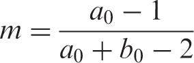
Hence, the a₀ (and consequently b₀) could be derived from:

(21)

For a non-informative prior, and then a Jeffrey’s prior could be used such that:

(22)

Note, the methodology described earlier in the article that accounts for the imprecision in control response could be considered to be sample calculations calculated under a Bayesian framework but with a non-informative prior distribution for θ.

5.4.2 Anticipated response

The anticipated control response is defined as $p_{C_{1}}$ . This could be taken as the response observed in a previous clinical trial. The control response equates to an observed number of successes (a₁) and failures (b₁).

5.4.3 Posterior response

With the anticipated and prior responses, the posterior distribution can be calculated from the following result:

(23)

These values for $I^{- 1} (perc, a_{1} + a_{0}, b_{1} + b_{0})$ can be used in (18) to obtain estimates of the sample size for a proportional difference, respectively, accounting for the imprecision in the variance estimate.

It is best to highlight the points through worked example.

5.4.4 Worked example 4 – simple Bayesian approach

We will now revisit the sample size calculations by applying Bayesian methods to try and obtain better estimates of the control response. As earlier, we will assume that the control response is 85% but that this was estimated from a study with 100 patients. Thus, in observed 85 successes (a₁ = 85) and 15 failures (b₁ = 15) we will undertake the calculations for three different priors as follows: a non-informative, a pessimistic and an optimistic.

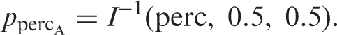
With a non-informative prior, a₁ = 85, b₁ = 15 and a₀ = 0.5 and b₀ = 0.5. The distributions of the different responses are given in Figure 1. The sample size is estimated to be 122 patients per arm. This is the same as calculated in Worked Example 3.

Figure 1.

Prior, likelihood and posterior responses for a non-informative prior: (a) non-informative prior, (b) likelihood function, (c) posterior and (d) all three together.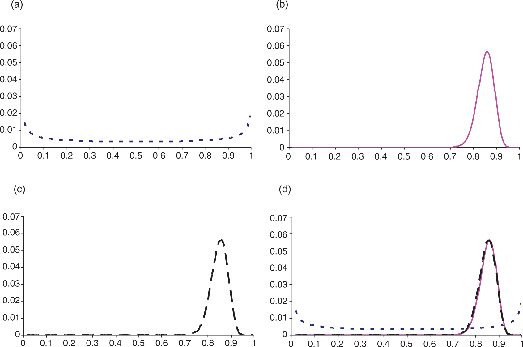

With a more pessimistic prior, the most likely response being 80% with 90% certainty being greater than 75%, a₁ = 85, b₁ = 15 and a₀ = 106.304 and b₀ = 27.326. The distributions for the different response are given in Figure 2. The sample size estimate is increased to 139 patients per arm.

Figure 2.

Prior, likelihood and posterior responses for a pessimistic prior: (a) pessimistic prior, (b) likelihood function, (c) posterior and (d) all three together.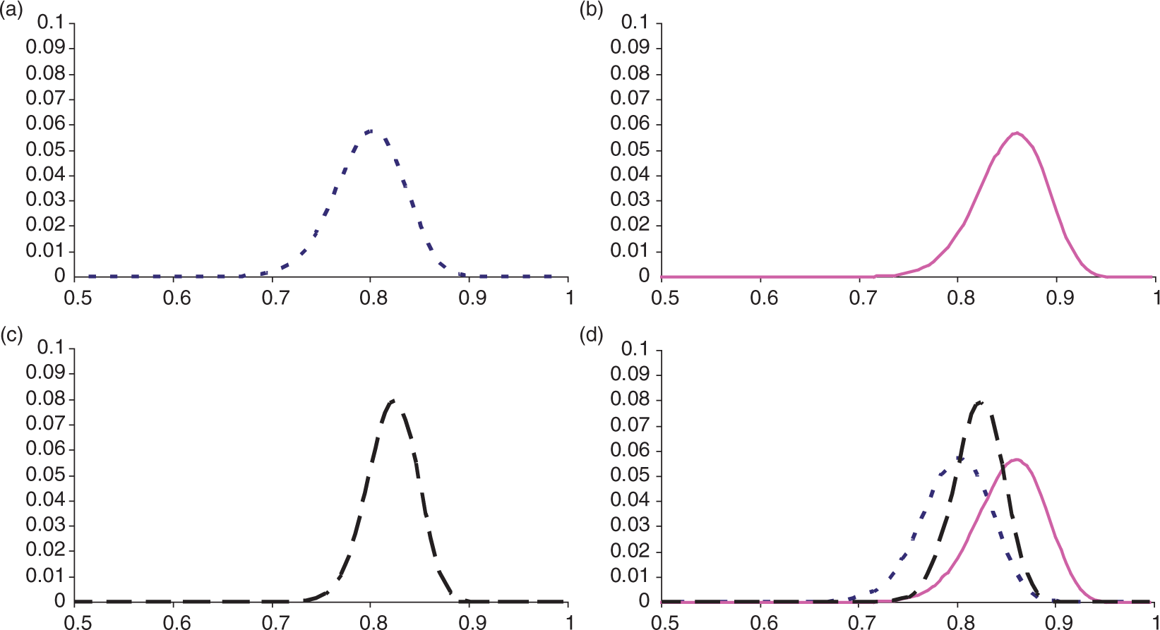

With a prior that the control response rate observed is about right, the most likely response being 85% with 90% certainty that is greater than 80%, a₁ = 85, b₁ = 15 and a₀ = 98.716 and b₀ = 18.244. The distributions for the responses are given in Figure 3. The sample size estimate is 122 patients per arm – the same again as with a non-informative prior.

Figure 3.

Prior, likelihood and posterior responses for an optimistic prior: (a) optimistic prior, (b) likelihood function, (c) posterior and (d) all three together.

5.5 Calculations taking account of the imprecision of the estimates of the population effects with respect to the assumptions about the risk difference and the variance used in the sample size calculations

When considering designing a non-inferiority study, the effect of the imprecision of the control p_C on the absolute risk difference as well as the variance may be of particular importance as p_C feeds into the assumptions both about the risk difference and the variance.

To allow for the imprecision in the estimation of the risk difference and variance, we could use numerical methods to calculate the sample size and the following result:

(24)

Note that a number of additional issues are now considered:

The investigative response rate, p_T, is assumed fixed – calculated from the initial p_C but not from individual $p_{{perc}_{C}}$ .

Following from 1, for instances where $p_{{perc}_{C}} - p_{T}$ exceeds the non-inferiority bound, then the power for this percentile (to be averaged across for power calculation) is set to 0.

Note, the methodology could be extended to allow both p_C and p_T to vary, but here, p_T is assumed fixed. That is, if a higher than expected response rate is to be observed, then this is going to be only on p_C making it difficult to declare non-inferiority.

5.5.1 Worked example 5 – accounting for the imprecision in the control response with respect to the risk difference

Previously, we estimated a sample size assuming the control and investigative responses to be 85%. However, the control response was estimated from a trial with just 100 patients. Repeating the sample calculations to account for the imprecision in the control response and how this may impact on the estimation of the risk difference and the variance, the sample size estimate is increased to 134 patients per arm.

5.6 Calculations that take account of the imprecision of the estimates effects with respect to the assumptions about the mean difference and the variance used in the sample size calculations – Bayesian methods

As previously discussed, the percentiles for a posterior control response can be calculated from the percentiles for p_C elicited to give an estimate of the sample size. Again, it is best to highlight the points through a worked example.

5.6.1 Worked example 6 – accounting for the imprecision in the control response with Bayesian approaches with respect to the risk difference

For the absolute difference scale with a non-informative prior, the sample size is estimated to be 134 patients per arm. This is the same as the sample size calculated earlier.

With a more pessimistic prior (the most likely response being 90% with 90% certainty being greater than 85%), the sample size estimate is increased to 166 patients per arm.

Note that this is more of a pessimistic prior than when just looking at variability. Here, a higher control response could equate to a narrowing of the effect of the investigative treatment over control. This will adversely affect the sample size.

With a prior that the control response rate observed is about right (the most likely response being 85% with 90% certainty and that it is greater than 80%), the sample size estimate is increased to 124 patients per arm.

6 Discussion

When calculating a sample size for a non-inferiority study, it is recommended to use the anticipated responses for the responses under the null hypothesis. Within the parameters of a simulation performed in the article, it was demonstrated that on an average these calculations gave the best results. If, however, we wished to have ‘at least’ the specified power, the same simulations demonstrated that the methodology using maximum likelihood estimates could be applied.

When designing a non-inferiority trial with high anticipated responses, the sample size estimate can be very sensitive to assumptions made with respect to the anticipated response. It is recommended when designing a study, at the very least, that a sensitivity analysis be performed on the assumptions made in the calculation. It is also recommended that the Bayesian methods described in this article be used to incorporate prior information and beliefs formally into the process of calculating the sample sizes.

We recognise that these calculations add to the complexity of the sample size calculations, but then a sample size estimate has considerable impact on the planning and budgeting of a trial. Clinical trials are expensive to conduct, and it is important to have as good an estimate of the sample size as possible and also to know that a trial is robust enough to the assumptions in a sample size calculation. We go by the maxim that one should spend at least the same amount of time designing a trial as one does for analysing it. After all, an incorrect analysis can be easily remedied with a correct analysis, whilst an incorrect design, specifically, for example, too small a sample size, cannot be remedied in some cases without running a new trial.

One point to be highlighted though is that despite these sample calculations being complex, they are still only providing a sample size estimate, and the sample size estimate is only as good as the estimates underpinning the calculation.

To specifically adjudicate on the quality anticipated control response rate, we recommend consideration be made to the following questions or points based on similar considerations for the variance for normal data.⁴

Was the design ostensibly similar to the one you are designing? On the basic level is the data from a randomised controlled trial – observational or other data with greater variability. If a multicentre trial is being undertaking, is the variance estimated also from a similarly designed trial? If the study was a pilot study, how would this affect the response rate? Was the time relative to treatment of the outcome of interest similar to your own?

Was the population similar to your own study you are planning? The most obvious consideration is to ask whether the demographics were the same, but if the trial conducted was a multicentre one, was it conducted in similar countries? Different countries may have different types of care (e.g., different concomitant medication) and so may have different trial populations. Was the same type of patient enrolled (the same mixed of mild, moderate and severe)?

Was the same statistical analysis undertaken? Not just the question of whether the same procedure was used for the analysis but were the same covariates fitted into the model?

If there are substantial doubts about the sample size calculation and you believe the study design is oversensitive to assumptions made in the calculation, then consideration should be made to some form of adaptive trial design including a sample size re-estimation.⁷ This is particularly an important consideration for an adaptive trial design where if the control response is higher (or lower), there can be a substantial impact on the study power even if the investigative response observed is as expected.

Footnotes

Appendix

Table A1.

Sample sizes for a non-inferiority study estimated through simulation and three alternative methods: Method 1 (using assumed responses), Method 2 (using anticipated responses in conjunction with the non-inferiority limit) and Method 3 (using maximum likelihood estimates) for 90% power and a Type I error rate of 2.5%

			Confidence interval method			Sample size method
				Wilson
π _A	π_A − π_B	Limit	Normal	Wilson	CC	Method 1	Method 2	Method 3
0.70	0.00	0.05	1765	1761	1770	1766	1763	1783
		0.10	441	441	441	442	439	452
		0.15	196	196	196	197	194	204
		0.20	110	110	115	111	108	116
	−0.05	0.05	423	418	418	418	418	423
		0.10	186	186	186	186	185	191
		0.15	109	104	104	105	103	109
		0.20	67	67	67	67	65	72
	−0.10	0.05	178	178	173	173	174	176
		0.10	102	102	97	98	98	101
		0.15	67	62	62	63	62	66
		0.20	43	43	43	44	43	47
	−0.15	0.05	89	94	89	89	91	92
		0.10	57	57	57	57	58	60
		0.15	39	44	39	40	40	43
		0.20	29	29	29	29	29	32
	−0.20	0.05	50	55	50	51	53	53
		0.10	35	35	35	36	37	37
		0.15	26	31	26	26	27	28
		0.20	20	20	20	20	20	23
0.75	+0.05	0.10	1667	1662	1676	1671	1662	1720
		0.15	418	414	423	418	412	438
		0.20	186	182	191	186	181	198
	0.00	0.05	1581	1572	1576	1577	1573	1597
		0.10	394	394	399	395	391	407
		0.15	175	175	175	176	172	185
		0.20	99	99	99	99	96	107
	−0.05	0.05	370	370	365	366	366	371
		0.10	167	167	167	163	162	169
		0.15	91	91	96	92	90	97
		0.20	63	58	63	59	57	64
	−0.10	0.05	152	152	147	148	149	150
		0.10	83	83	83	83	83	87
		0.15	53	53	53	54	53	57
		0.20	37	37	37	37	36	41
	−0.15	0.05	73	78	78	73	75	75
		0.10	47	47	47	47	48	49
		0.15	32	37	37	33	33	36
		0.20	24	29	29	24	24	28
0.80	+0.10	0.15	1555	1546	1566	1556	1540	1567
	+0.05	0.10	1466	1457	1466	1466	1452	1524
		0.15	365	361	370	366	359	392
	0.00	0.05	1350	1345	1345	1346	1342	1369
		0.10	336	341	341	337	334	352
		0.15	149	149	154	150	147	162
	−0.05	0.05	302	302	302	303	303	308
		0.10	139	139	139	135	134	141
		0.15	76	76	81	76	74	83
	−0.10	0.05	117	117	1177	117	118	119
		0.10	66	66	71	66	66	70
		0.15	42	47	47	43	42	47
0.85	+0.10	0.15	1329	1320	1335	1324	1309	1461
	+0.05	0.10	1213	1213	1219	1209	1199	1290
		0.15	307	302	307	303	296	337
	0.00	0.05	1077	1077	1077	1072	1069	1099
		0.10	268	273	273	268	265	287
		0.15	124	124	124	120	116	135
	−0.05	0.05	229	234	234	229	229	234
		0.10	102	107	107	102	101	110
		0.15	58	62	62	58	56	66
0.90	+0.05	0.10	919	925	925	915	905	1022
	0.00	0.05	757	768	762	757	754	791
		0.10	189	200	200	190	186	215

References

CHMP. Points to Consider on Switching Between Superiority and Non-inferiority (Doc CPMP/EWP/482/99), http://www.tga.gov.au/docs/pdf/euguide/ewp/048299en.pdf (accessed January 2010).

ICH E10. Choice of control group in clinical trials, http://www.ich.org/LOB/media/MEDIA486.pdf (accessed January 2010).

CHMP. Guideline for the choice of non-inferiority margin, http://www.emea.europa.eu/pdfs/human/ewp/215899en.pdf (accessed January 2010).

Julious

. Tutorial in biostatistics: sample sizes for clinical trials with normal data. Statistics in Medicine 2004; 23: 1921–1986.

Jones

Jarvis

Lewis

Ebbutt

. Trials to assess equivalence: the importance of rigorous methods. British Medical Journal 1996; 313: 36–39.

Morikawa

Yoshida

. A useful testing strategy in phase III trials: combined test of superiority and test of equivalence. Journal of Biopharmaceutical Statistics 1995; 5(3): 297–306.

Julious

. Sample sizes for clinical trials 2009 Abingdon, England: Chapman and Hall.

Chan

ISF

. Proving non-inferiority or equivalence of two treatments with dichotomous endpoints using exact methods. Statistical Methods in Medical Research 2003; 12: 37–58.

Chen

Tsong

Kang

. Tests for equivalence or non-inferiority between two proportions. Drug Information Journal 2000; 34: 569–578.

10.

ICH E9. Statistical principles for clinical trials, http://www.ich.org/LOB/media/MEDIA485.pdf (accessed January 2010).

11.

Newcombe

. Two-sided confidence intervals for the single proportion: comparison of seven methods. Statistics in Medicine 1998; 17: 857–872.

12.

Fleiss

. Statistical methods for rates and proportions 1981 2. New York: Wiley.

13.

Wilson

. Probable inference, the law of succession and statistical inference. Journal of the American Statistical Association 1927; 22: 202–212.

14.

Dunnett

Gent

. Significance testing to establish equivalence between treatments, with special reference to data in the form of 2×2 tables. Biometrics 1977; 33: 593–602.

15.

Farrington

Manning

. Test statistics and sample size formulae for comparative binomial trials with null hypothesis of non-zero risk difference or non-unity relative risk. Statistics in Medicine 1990; 9: 1447–1454.

16.

SAS Institute Inc. SAS 9.1.3 help and documentation 2000–2004; Cary, NC: SAS Institute Inc.

17.

Chan

ISF

. Proving non-inferiority or equivalence of two treatments with dichotomous endpoints using exact methods. Statistical Methods in Medical Research 2003; 12: 37–58.

18.

CPMP. Notes for guidance on the evaluation of medicinal products indicated for the treatment of bacterial infections (Doc CPMP/EWP/558/95), http://www.emea.europa.eu/pdfs/human/ewp/055895en.pdf (accessed January 2010).