On weighting approaches for missing data

Abstract

We review the class of inverse probability weighting (IPW) approaches for the analysis of missing data under various missing data patterns and mechanisms. The IPW methods rely on the intuitive idea of creating a pseudo-population of weighted copies of the complete cases to remove selection bias introduced by the missing data. However, different weighting approaches are required depending on the missing data pattern and mechanism. We begin with a uniform missing data pattern (i.e. a scalar missing indicator indicating whether or not the full data is observed) to motivate the approach. We then generalise to more complex settings. Our goal is to provide a conceptual overview of existing IPW approaches and illustrate the connections and differences among these approaches.

Keywords

inverse probability weighting missing at random missing data monotone missing missing not at random non-monotone missing

1 Introduction

Interest in the use of secondary healthcare databases (e.g. administrative claims, electronic health records (EHRs) and cancer registries) for medical research is increasing, partially because these data are readily available, relatively inexpensive to access and cover large representative populations. However, these databases are collected for non-research purposes. For example, administrative and medical claims databases are assembled for the purposes of administering, billing and reimbursing healthcare services. Moreover, patients in clinical practice settings are not monitored as closely as those in clinical trials. In consequence, a substantial fraction of the needed data is missing for some subjects. These data issues pose analytic challenges and raise validity concerns.

By design, each of these secondary databases may contain only a subset of the variables of interest. For example, administrative claims data contain information on healthcare insurance membership, drug coverage, healthcare utilisations (i.e. diagnosis and procedure codes) and medication dispensing records. But more detailed clinical information (e.g. BMI, vital signs and laboratory tests results) are recorded in EHR. For cancer patients, the cancer stage and histology information are recorded in cancer registries. As a consequence, systematic missing data occurs for some study participants for whom the data in certain databases are unavailable. Even for those with linked databases, missing data may still occur for reasons such as missed office visits, loss to follow-up, switch of healthcare systems and coding errors. Thus, failure to appropriately handle missing data may lead to inefficient or even invalid use of available data sources.

The simplest and most commonly used method to deal with missing data is the complete case approach in which standard analyses are applied to subjects with complete data on relevant variables. However, this analysis is biased unless the complete cases are representative of the study population (i.e. the data is missing complete at random, MCAR). This MCAR assumption rarely holds in medical applications.¹

More advanced statistical methods have been developed in the past decades to deal with missing data under less restrictive missing data mechanisms,² i.e. missing at random (MAR) and missing not at random (MNAR). MAR means the probability of missingness does not depend on unobserved elements conditional on observed data.³ MNAR indicates settings in which neither MCAR nor MAR holds. In this article, we review a class of approaches for missing data – the inverse probability weighting (IPW) approaches. The intuitive idea is to create weighted copies of the complete cases to remove selection bias introduced by missing data processes. The weighting idea originates in the survey sampling literature.⁴ It has been further generalised by Robins, Rotnitzky, and others to address a variety of important issues such as confounding bias in observational studies and bias due to missing data.^5–8 Alternatives to IPW include parametric likelihood inference,^9–11 parametric Bayesian inference^12–14 and parametric multiple imputation^15–17 inference.

We introduce and illustrate the class of IPW approaches for three missing data patterns, uniform missingness, monotone missingness and non-monotone missingness. For each pattern, we consider both MAR and MNAR mechanisms. We begin with relatively simple scenarios, and then generalise to more complex settings. Due to space limitations, we do not dwell on mathematical details but refer the interested readers to the original journal articles or to the books by Tsiatis or van der Laan and Robins.^18,19

This article is organised as follows. In Section 2, we introduce the notation and models needed to formalise the missing data patterns and mechanisms we consider. We also introduce four motivating examples. In Section 3, we motivate the weighting approaches by demonstrating the bias in the complete case approach when MCAR does not hold. In Sections 4–6, we introduce weighting approaches for our three missing data patterns. We conclude with a discussion.

2 Models and notations

We let ${L_{i} = (W_{i}^{T}, V_{i}^{T})^{T}, i = 1, \dots, n}$ denote the full data on the n study subjects, where the p-dimensional vector $W_{i} = (W_{1, i}, \dots, W_{p, i})^{T}$ denotes the variables that are always observed for each subject i and the q-dimensional vector $V_{i} = (V_{1, i}, \dots, V_{q, i})^{T}$ denotes the variables that are subject to missingness. We let $R_{i} = (R_{1, i}, \dots, R_{q, i})^{T}$ denote the vector of missing indicators for subject i where the sth element $R_{s, i}$ ( $1 \leq s \leq q$ ) equals 1 if $V_{s, i}$ is observed, and 0 otherwise. Let $V_{(R_{i}), i}$ denote the observed components of $V_{i}$ . Let $O_{i} = (R_{i} {, L}_{obs, i} = (W_{i}^{T}, V_{(R_{i}), i}^{T})^{T})$ denote the observed data for subject i and let $L_{mis, i} = V_{(1 - R_{i}), i}$ denote the unobserved components of $V_{i}$ . Here $1$ denotes a vector of 1’s. This notation can be used to represent a wide class of missing data patterns. For example, in a missing outcome model, W represents a vector of covariates and V is the outcome of interest Y. The parameter of interest might be the marginal outcome mean $E [Y]$ or the coefficients β in an outcome regression model $E [Y | W; β]$ . In missing data models with missing outcome and covariates, W would represent the covariates that are always observed and V would include both the outcome of interest and the covariates that are subject to missingness.

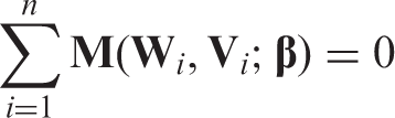
Throughout we assume that $(W_{i}, V_{i}, R_{i})$ , $i = 1, \dots, n$ are independent and identically distributed random vectors. We assume the parameter of interest $β^{*}$ is the unique solution to the equation $E [M (W_{i}, V_{i}; β^{*})] = 0$ , where $M (W_{i}, V_{i}; β)$ is a known m-dimensional function of the full data $(W_{i}, V_{i})$ and a parameter β, $β^{*}$ is the true value of β, and the expectation is under the distribution of $(W_{i}, V_{i})$ . Thus, $M (W_{i}, V_{i}; β)$ is an unbiased estimating function for $β^{*}$ . Here $β^{*}$ is a functional of the distribution of the full data $(W_{i}, V_{i})$ .

We consider the following three missing data patterns: uniform missingness, monotone missingness and non-monotone missingness. The weighting approach applies equally to all. However, its implementation is much more complicated for non-monotone missing data patterns. We will start with a simple uniform missing pattern to illustrate and motivate the basic idea.

2.1 Missing pattern 1: uniform missing data, i.e. $R_{1} = " P 427 A 97 56 . . . = " P 427 A 97 56 R_{q} = " P 427 A 97 56 R$

Under uniform missingness, either the entire vector $V_{i}$ is observed for subject i or it is completely missing. This pattern often occurs when information is extracted from multiple data sources. For example, administrative claims data contain information on basic demographics (age, gender), healthcare utilisations and medication dispensing records. However, more detailed clinical information such as vital signs and lab test results would be available only for a subset of the study participants with linked EHR data.

2.2 Motivating example 1

Consider a hypothetical study evaluating the 1-year incidence rate of heart disease among new users of non-steroidal anti-inflammatory drugs. Data are extracted from a health insurance administrative claims database which contains information on medication dispensing records and disease diagnosis history. The indicator variable $V = Y$ indicates whether heart disease occurred during the 1-year follow-up period after drug initiation. Let $β^{*} = E [Y]$ . Then $M (Y; β)$ is $Y - β$ . The outcome will be missing in participants who dis-enroll from the insurance plan during the follow-up period. The vector of covariates W includes demographics (age, gender), geographic region, geographically derived socioeconomic status and comorbidity conditions.

2.3 Missing pattern 2: monotone missing data

Under monotone missingness, if the sth element ( $R_{s} = 0$ ) of $V_{i}$ is missing then all subsequent elements are missing ( $R_{t} = 0$ for any $s < t \leq q$ ). This pattern occurs frequently in longitudinal studies with repeated measurements in which subjects who drop out of the study never re-enter. Then V_s might denote the data that were to be collected at the sth planned clinic visit. Even if some subjects return after missing one or more visits, one can choose to make the data ‘monotone’ for purposes of data analysis by choosing to ignore in the analysis any data recorded subsequent to a missing visit. Note uniform missing data is actually a special case of monotone missing data.

2.4 Motivating example 2

Consider an observational study to compare the effects of two anti-hypertensive agents (e.g. angiotensin-converting enzyme inhibitors and beta-blockers) on reducing blood pressure (BP) level among incident users. The study participants were identified using claims and EHR data. Then W contains the treatment indicator and some baseline covariates (e.g. age, sex and comorbidity conditions). The vector V contains two elements; V₁ records the baseline BP and $V_{2} = Y$ records the BP at the end of a 12-month follow-up period. The baseline BP V₁ is incomplete as some patients do not have EHR data available or did not have their BP measured during the baseline period. Similarly, some subjects have $V_{2} = Y$ missing. We decide to make the data ‘monotone’ by ignoring the data on V₂ for subjects missing V₁. Suppose we are interested in the coefficient β in the regression model $E [Y | W, V_{1}; β] = b (W, V_{1}; β) = (W^{T}, V_{1}) β$ . We would take $M (W, V; β) = [Y - b (W, V_{1}; β)] (\binom{W}{V_{1}})$ .

2.5 Missing pattern 3: non-monotone missing data

Non-monotone missingness refers to any missing data pattern that is not monotone. Thus, we may have $R_{t} = 1$ but $R_{s} = 0$ for some subjects and $R_{t} = 0$ but $R_{s} = 1$ for others. This is the most complicated missing data pattern. We consider two motivating examples for this pattern.

2.6 Motivating example 3

Consider a regression analysis with missing covariates. Suppose we are interested in identifying predictors of episodes of exacerbation for children with persistent asthma. The study cohort of children with persistent asthma was identified using healthcare claims data. The vector W, ascertained from claims data, includes data on demographic characteristics and a binary outcome encoding 2 or more ER visits for asthma during a 12-month study period. Surveys were mailed to parents to obtain data on a baseline asthma severity score (V₁), household income (V₂) and a measure of the parents’ expectation on child functioning with asthma (V₃). Parents may answer none, one, two or three of the three questions. This missing pattern is non-monotone. We are interested in the regression parameter $β^{*}$ in a logistic regression model regressing the outcome on potential predictors. The estimating equation $M (W, V; β)$ is the score function for β.

2.7 Motivating example 4

Consider a longitudinal follow-up study with repeated measurements of BP at three time points, $s = 1, 2, 3$ . As before, W contains the treatment indicator and baseline covariates (e.g. age and sex). Let $V_{s, i}$ indicate the BP measured at the sth time point and $V_{i} = (V_{1, i}, V_{2, i}, V_{3, i})^{T}$ . Unlike in example 2, we do not ignore subsequent data on subjects missing V₁ or V₂. Thus, this missing pattern is non-monotone. We are interested in the mean of $V_{i}$ , $β^{*} = E [V_{i}]$ . Thus, $M (W, V; β) = V - β$ .

For each missing pattern, we consider both MAR and MNAR data generating processes.³ Data are said to be MAR if the conditional missing probabilities given the full data do not depend on the unobserved components of V, i.e.

P (R_{i} = r | W_{i}, V_{i}) = P (R_{i} = r | L_{obs, i} = (W_{i}, V_{(r), i}))

(1)

In the special case of MCAR, $P (R_{i} = r | W_{i}, V_{i})$ is constant. Let γ denote the parameters governing the missing data process and θ denote the parameters governing the distribution of the full data $L = (W, V)$ , and assume they are variation independent. Then under MAR, the likelihood $f (O_{i}, γ, θ)$ of the observed data factors into a component $Pr (R_{i} = r | L_{obs, i}; γ)$ depending on γ alone and a component $f (L_{obs, i}; θ)$ depending on θ alone. Thus, MAR is referred to as ignorable missingness because the missing data process can be ‘ignored’ in likelihood-based inference on a parameter $β^{*}$ that are functions of the parameters θ governing the marginal distribution of the full data L. The IPW approach takes a different perspective than likelihood-based approaches by using estimates of the missing data process to derive valid inferences on the parameter of interest $β^{*}$ .

When MAR fails to hold, the missing data mechanism is said to be MNAR or non-ignorable, i.e. the missing probabilities depend on unobserved components of V conditional on observed data. In this setting, the parameter of interest is typically unidentifiable unless additional assumptions on the missing data process are imposed. These assumptions usually are investigator specified and cannot be empirically tested when the full data model is non-parametric. Therefore, it is a common practice to conduct a sensitivity analysis in which we vary these additional assumptions over a plausible range and examine how inferences on $β^{*}$ change. As we will show next, weighting approaches in MAR settings can be naturally extended to MNAR settings by specifying a selection bias function to quantify the residual association of the missing probabilities and unobserved components of V after adjusting for observed data. Sensitivity analysis can then be conducted by varying the parameters in the selection bias function and/or the functional form.

We let $π_{i} (W_{i}, V_{i}, r)$ denote the conditional missing probability $P (R_{i} = r | W_{i}, V_{i})$ . Throughout we assume that $P (R_{i} = 1 | W_{i}, V_{i}) > 0$ with probability 1.

3 Why the complete case approach may be biased?

We first illustrate why the complete case approach may be biased when MCAR does not hold.¹⁰ If the full data were observed, $β^{*}$ could be estimated by solving

\sum_{i = 1}^{n} M (W_{i}, V_{i}; β) = 0

(2)

the empirical version of

E [M (W_{i}, V_{i}; β)]

. Unfortunately, when missing data exist, the solution to Equation (2) depends on unobserved components of V. Suppose

E [M (W_{i}, V_{i}; β^{*})] = 0

, but

E [M (W_{i}, V_{i}; β^{*}) | R_{i} = 1] \neq 0

, then if we use complete cases only and estimate

β^{*}

by solving the estimating equation

\sum_{i = 1}^{n} I (R_{i} = 1) M (W_{i}, V_{i}; β) = 0

, it is obvious that the solution to the equation above,

{\tilde{β}}_{cc}

, may be biased unless

E [P (R_{i} = 1 | W_{i}, V_{i}) M (W_{i}, V_{i}; β^{*})] = 0

, e.g.

P (R_{i} = 1 | W_{i}, V_{i})

is constant.

Heuristically, when MCAR fails to hold, the complete cases are a selected, non-random subsample of the study population. Thus, inference obtained by applying standard approaches to the complete cases may be biased for $β^{*}$ . The IPW approach restores unbiasedness by creating a pseudo-population in which selection bias due to the missing data is removed. We next introduce the IPW methods for the three missing data patterns respectively.

4 Uniform missing pattern

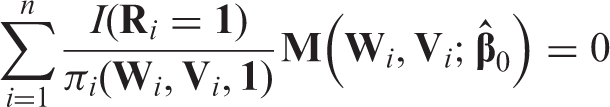
A uniform missing data pattern is a pattern in which the missing indicator vector R takes only two possible values $1 = (1, 1, \dots, 1, \dots 1)^{T}$ or $0 = (0, 0, \dots 0, \dots 0)^{T}$ . Noted above, unless MCAR holds, the complete case approach is likely biased. To remove selection bias due to missing data, the IPW approach weights each subject i with complete data ( $R_{i} = 1$ ) by the inverse of the conditional probability of observing the full data $π_{i} (W_{i}, V_{i}, 1)$ . For illustration, we temporarily assume $π_{i} (W_{i}, V_{i}, 1)$ is a known function of $(W_{i}, V_{i})$ as is the case in studies with missingness by design (e.g. studies with two-stage sampling). Then, the simple IPW estimator ${\hat{β}}_{0}$ solves the following estimating equation²⁰

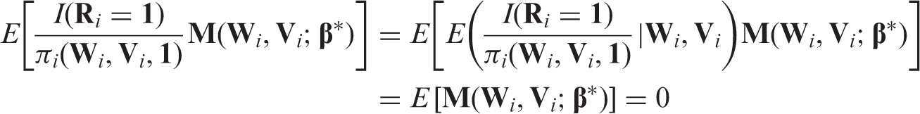
\sum_{i = 1}^{n} \frac{I (R_{i} = 1)}{π_{i} (W_{i}, V_{i}, 1)} M (W_{i}, V_{i}; {\hat{β}}_{0}) = 0

(3)

Under regularity conditions, ${\hat{β}}_{0}$ is a consistent estimator of $β^{*}$ since

\begin{matrix} E [\frac{I (R_{i} = 1)}{π_{i} (W_{i}, V_{i}, 1)} M (W_{i}, V_{i}; β^{*})] = E [E (\frac{I (R_{i} = 1)}{π_{i} (W_{i}, V_{i}, 1)} | W_{i}, V_{i}) M (W_{i}, V_{i}; β^{*})] \\ = E [M (W_{i}, V_{i}; β^{*})] = 0 \end{matrix}

Note that the above equalities hold regardless of whether or not the missingness is ignorable (i.e. MAR or MNAR). In addition, a fully parametric model for the full data is not required. Under mild conditions, the solution to Equation (3) is a consistent and asymptotically normal (CAN) estimator of $β^{*}$ .²⁰

This IPW estimator ${\hat{β}}_{0}$ demonstrates the fundamental principle of the weighting approach; weighted copies of complete cases remove the selection bias introduced by the missing data process. However, note Equation (3) depends only on data from complete cases. Then, ${\hat{β}}_{0}$ is not fully efficient. To increase efficiency, we can add to the estimating equation augmentation terms. These terms depend on data from both complete and incomplete cases.

From the definition of $π_{i} (W_{i}, V_{i}, 1)$ , it is clear that an augmentation term $A_{i} (ϕ)$ that takes the form $(I (R_{i} = 1) π_{i} (W_{i}, V_{i}, 1)^{- 1} - 1) ϕ (W_{i})$ has mean zero, where $ϕ (W_{i})$ is an m-dimensional vector of arbitrary functions of the always observed variables $W_{i}$ . Let $D_{i} (β, ϕ)$ be $I (R_{i} = 1) / π_{i} (W_{i}, V_{i}, 1) M (W_{i}, V_{i}; β) - A_{i} (ϕ)$ . Then, $D_{i} (β, ϕ)$ is mean zero at $β^{*}$ and the solution ${\hat{β}}_{ϕ}$ to $\sum_{i = 1}^{n} D_{i} (β, ϕ) = 0$ is a consistent estimator of $β^{*}$ under regularity conditions.²¹ Moreover, the asymptotic variance of ${\hat{β}}_{ϕ}$ equals Γ $Γ^{- 1} var [D_{i} (β^{*}, ϕ)] Γ^{- 1, T}$ where Γ $Γ \equiv E [\partial M (W_{i}, V_{i}; β) / \partial β^{T} | β = β^{*}]$ . This implies that the choice of ϕ affects the efficiency of ${\hat{β}}_{ϕ}$ only through the term $var [D_{i} (β, ϕ)]$ . By simple algebra, one can easily show that

D_{i} (β, ϕ) = M (W_{i}, V_{i}; β) + (\frac{I (R_{i} = 1)}{π_{i} (W_{i}, V_{i}, 1)} - 1) (M (W_{i}, V_{i}; β) - ϕ_{i})

and

$var [D_{i} (β, ϕ)] = var [M (W_{i}, V_{i}; β)] + var [(I (R_{i} = 1) / π_{i} (W_{i}, V_{i}, 1) - 1) (M (W_{i}, V_{i}; β) - ϕ_{i})]$ as the two terms in the above representation of $D_{i} (β, ϕ)$ are uncorrelated. We want to select ϕ so that $var [D_{i} (β, ϕ)] \leq var [D_{i} (β, ϕ = 0)]$ for any $M (W_{i}, V_{i}; β)$ . Since the first term in $var [D_{i} (β, ϕ)]$ does not depend on ϕ, we need to select ϕ such that $var [(I (R_{i} = 1) π_{i} (W_{i}, V_{i}, 1)^{- 1} - 1) (M (W_{i}, V_{i}; β) - ϕ_{i})] < / inline - graphic >$ $\leq var [(I (R_{i} = 1) π_{i} (W_{i}, V_{i}, 1)^{- 1} - 1) M (W_{i}, V_{i}; β)]$ . The inequality above is satisfied when $A_{i} (ϕ)$ = $(I (R_{i} = 1) π_{i} (W_{i}, V_{i}, 1)^{- 1} - 1) ϕ (W_{i})$ is the projection of $(I (R_{i} = 1) π_{i} (W_{i}, V_{i}, 1)^{- 1} - 1) M (W_{i}, V_{i}; β)$ onto a subspace $Λ_{sub}$ of $Λ_{1} \equiv {(I (R_{i} = 1) π_{i} (W_{i}, V_{i}, 1)^{- 1} - 1) h (W_{i}) : h \in L_{2} (f (W))}$ , as the norm of the residual from a projection is smaller than or equal to the norm of the original vector. For a given $M (W_{i}, V_{i}; β)$ , the most efficient augmentation term, $ϕ_{eff}$ , is obtained by projecting $[I (R_{i} = 1) π_{i} (W_{i}, V_{i}, 1)^{- 1} - 1] M (W_{i}, V_{i}; β)$ onto the entire space $Λ_{1}$ . With uniform missing patterns, when MAR holds, $ϕ_{eff}$ equals $E [M | R = 1, W]$ . For example, in our motivating example 1, $M = Y - β$ and thus $ϕ_{eff} = E [Y | R = 1, W] - β$ . See references for technical details.^6,19–30

So far we have assumed that $π_{i} (W_{i}, V_{i}, 1)$ is known, i.e. missingness by design, which occurs infrequently in medical applications. Therefore, we need to estimate $π_{i} (W_{i}, V_{i}, 1)$ using the observed data. We next discuss strategies to obtain estimated missing probabilities ${\hat{π}}_{i} (W_{i}, V_{i}, 1)$ under MAR and MNAR mechanisms respectively.

4.1 Missing at random

Under MAR, by Equation (1), $π_{i} (W_{i}, V_{i}, 0)$ depends on $W_{i}$ only since $V_{(0), i}$ is an empty set. Thus $π_{i} (W_{i}, V_{i}, 1)$ also depends only on $W_{i}$ since $π_{i} (W_{i}, V_{i}, 1) = 1 - π_{i} (W_{i}, V_{i}, 0)$ . In other words, for $r \in {1, 0}$ , $P (R_{i} = r | W_{i}, V_{i}) = P (R_{i} = r | W_{i})$ . Since $(R_{i}, W_{i})$ is observed for each subject i, then the estimated conditional missing probability ${\hat{π}}_{i} (W_{i}, r)$ can be obtained by regressing the missing indicator $R_{i}$ on the always observed covariates $W_{i}$ via either a parametric regression model (e.g. logistic regression) or non-parametric, data-adaptive algorithms (e.g. tree-based methods).^31–35

In many studies that obtain data from electronic medical databases, the number of covariates that need to be adjusted for to make the MAR assumption plausible is quite large.³⁶ Then it will be difficult to impose a correct parametric model for $P (R_{i} = 1 | W_{i})$ due to the curse of dimensionality. A mis-specified parametric model may result in significantly biased results. Data-adaptive, tree-based methods provide promising alternatives.^32,33,35 They are designed to minimise the mean squared prediction error, no matter how many covariates need to be adjusted for. The methods are easy to implement with minimum analyst input. Trees have many advantages including being robust to outliers, insensitive to covariate transformation, and the ability to capture complex interactions and highly correlated variables. See Hastie et al.³⁵ and Therneau and Atkinsoon³⁷ for a comprehensive review of the method and software programs.

After ${{\hat{π}}_{i} (W_{i}, 1), i = 1, \dots, n}$ are obtained, the IPW estimator ${\hat{β}}_{0}$ is obtained by solving equation (3), with ${\hat{π}}_{i} (W_{i}, 1)$ substituted for $π_{i} (W_{i}, 1)$ . To obtain the efficient augmented IPW estimators ${\hat{β}}_{ϕ_{eff}}$ , additional modelling and estimation are needed since $ϕ_{eff}$ depends on the unknown outcome regression function $E [M | R = 1, W]$ . In example 1, $ϕ_{eff} = E [Y | R = 1, W] - β$ . We use the complete cases to estimate $E [Y | R = 1, W]$ . As before, we can use either a parametric working model $E [Y | R = 1, W; ξ]$ or data-adaptive, tree-based regression techniques. After all the unknown functions and parameters are estimated, the augmented estimator ${\hat{β}}_{ϕ_{eff}}$ is obtained by solving the augmented estimating equation $\sum_{i = 1}^{n} D_{i} (β, {\hat{π}}_{i}, {\hat{ϕ}}_{eff}) = 0$ . In this example 1,

{\hat{β}}_{ϕ_{eff}} = \frac{1}{n} \sum_{i = 1}^{n} {\frac{I (R_{i} = 1)}{{\hat{π}}_{i} (W_{i}, 1)} Y_{i} - (\frac{I (R_{i} = 1)}{{\hat{π}}_{i} (W_{i}, 1)} - 1) \hat{E} [Y_{i} | R_{i} = 1, W_{i}]} .

It is worth noting that ${\hat{β}}_{ϕ_{eff}}$ is doubly robust (DR) in the sense that it is consistent for $β^{*}$ if either the working model for the missing data process $π (W_{i}, 1)$ or the working model for the outcome regression function $E [Y | R = 1, W]$ is correctly specified, but not necessarily both.³⁸ This nice property offers analysts two chances of making correct inference. Furthermore, the specified working models are practically certain to be incorrect especially in the presence of high-dimensional covariates. But as long as at least one model is nearly correct, the bias of ${\hat{β}}_{ϕ_{eff}}$ will be small by theory and simulation results.³⁸ The variance estimates of ${\hat{β}}_{ϕ_{eff}}$ can be obtained using either the asymptotic theory and delta methods or bootstrap re-sampling approaches.

4.2 Missing not at random

The MAR assumption cannot be empirically tested using observed data except under limited scenarios.³⁹ Subject matter expertise is usually required to judge its plausibility. When MAR does not appear to be reasonable, then additional assumptions on the missing data process need to be imposed to make the parameters of interest identifiable. Since these additional assumptions are not verifiable under a non-parametric full data model for $(W, V)$ , a sensitivity analysis is recommended. There are different ways of conducting a sensitivity analysis for MNAR (i.e. non-ignorable) data. We focus on the selection bias function approach for IPW estimators.^27,30 This approach decomposes the non-ignorable missing data process in a natural and straightforward manner, and thus makes it relatively easy to impose sensitivity assumptions using background information and substance knowledge.

Under MNAR, $π_{i} (W_{i}, V_{i}, 0)$ depends on both $W_{i}$ and $V_{i}$ . The selection bias function approach uses a user-specified function to quantify the residual association between the missingness probability and the possibly unobserved components of V conditioning on observed data. Specifically, we assume that

\frac{π_{i} (W_{i}, V_{i}, 0)}{π_{i} (W_{i}, V_{i}, 1)} = \frac{P (R_{i} = 0 | W_{i}, V_{i})}{P (R_{i} = 1 | W_{i}, V_{i})} = \exp {h (W_{i}) + q (W_{i}, V_{i})}

(4)

where

h (W_{i})

is an unrestricted function of

W_{i}

and

q (W_{i}, V_{i})

is the selection bias function. In other words, the ‘odds’ of having missing data depends on the possibly unobserved components

V_{i}

through the selection bias function

q (W_{i}, V_{i})

. Note that

q (W_{i}, V_{i})

needs to be specified by investigators, e.g.

q (W_{i}, V_{i}; c) = c^{T} V_{i}

where c is a given constant vector. When the model for the full data is non-parametric, the functional form chosen for

q (W_{i}, V_{i})

and the value of the parameter c are not empirically testable. In this article, we do not dwell on the choice of the selection bias function

q (W_{i}, V_{i})

as it depends heavily on the study setting and existing substance knowledge about the missing mechanism.^27,30

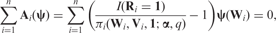
Assuming equation (4) holds and $q (W_{i}, V_{i})$ has been specified, we still need to estimate $h (W_{i})$ to obtain an estimated missing probability ${\hat{π}}_{i} (W_{i}, V_{i}, 1)$ . To do so, we usually impose a parametric working model $h (W_{i}; α)$ indexed by a unknown parameter α, e.g. $h (W_{i}; α) = α^{T} W_{i}$ . If W is categorical and the sample size is large, then we can use a saturated model to avoid model mis-specification. The parameter estimate $\hat{α}$ is obtained by solving the unbiased estimating equation

\sum_{i = 1}^{n} A_{i} (ψ) = \sum_{i = 1}^{n} (\frac{I (R_{i} = 1)}{π_{i} (W_{i}, V_{i}, 1; α, q)} - 1) ψ (W_{i}) = 0,

where

π_{i} (W_{i}, V_{i}, 1; α, q) = [1 + \exp {h (W_{i}; α) + q (W_{i}, V_{i})}]^{- 1}

and ψ is a vector of selected functions of

W_{i}

(e.g.

ψ (W_{i}) = W_{i}

). Note that the dimension of ψ needs to be equal to the dimension of α. Under regularity conditions, the corresponding

\hat{α}

is consistent for the true value

α^{*}

as long as the parametric working model is correct and equation (4) holds. However, the variance of

\hat{α}

depends on ψ.

As with MAR settings, the IPW estimator ${\hat{β}}_{0}$ can be obtained as the solution to equation (3) using the estimated missing probability ${\hat{π}}_{i} (W_{i}, V_{i}, 1) = π_{i} (W_{i}, V_{i}, 1; \hat{α}, q)$ . See references^27,28,40 for details on doubly-robust estimators and other, more efficient augmented estimators.

5 Monotone missing pattern

We now introduce the weighting approach for monotone missing patterns. Without loss of generality, we assume $R_{s, i} \geq R_{t, i}$ for any $1 \leq s < t \leq q$ . Equivalently, for each subject i, if the sth element $V_{s, i}$ is missing, then all subsequent elements ${V_{t, i} : t > s}$ are missing.

We first focus on example 2 and then present general results. Specially, we consider the setting in which $W_{i}$ contains the treatment indicator and a vector of baseline covariates that are recorded for each subject (e.g. age, sex and comorbidity conditions); while $V_{i} = (V_{1, i}, Y_{i})^{T}$ denotes the BP measured at baseline and at 12 months. We make the data ‘monotone’ by ignoring $Y = V_{2}$ on subjects missing V₁ ( $R_{2, i} = 0$ if $R_{1, i} = 0$ ). 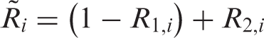We will estimate the coefficients β in the outcome regression model $E [Y | W, V_{1}; β] = b (W, V_{1}; β) = (W^{T}, V_{1}) β$ with $M (W, V; β) = [Y - b (W, V_{1}; β)] (\binom{W}{V_{1}})$ .

Monotone missing data can be analysed by applying the weighting approach for a uniform missing pattern in a nested fashion; that is, a monotone missing pattern can be decomposed into multiple uniform missing data models. For example, in example 2, since we have two missing components, we derive our estimators in two steps. In the first step, we derive estimators under an artificial missing data model in which the full data is $L_{i} = (W_{i}^{T}, V_{i}^{T})^{T}$ but the observed data is $O_{i}^{♦} = (W_{i}^{T}, R_{1, i}, R_{1, i} V_{1, i}, R_{1, i} Y_{i})^{T}$ . That is, both $V_{1, i}$ and Y_i are observed whenever the missing indicator $R_{1, i}$ is 1. In the second step, we consider a second artificial missing data model with $O_{i}^{♦}$ now the full data and $O_{i} = (W_{i}, R_{1, i}, R_{2, i}, R_{1, i} V_{1, i}, R_{2, i} Y_{i})$ the observed data. Our final estimator will only depend on the actual data ${O_{i}, i = 1, \dots, n}$ .

Specifically, let $E_{1, i} = e_{1, i} (W_{i}, V_{1, i}, Y) \equiv P (R_{1, i} = 1 | W_{i}, V_{1, i}, Y_{i})$ and $E_{2, i} = e_{2, i} (W_{i}, V_{1, i}, Y_{i}) \equiv P (R_{2, i} = 1 | R_{1, i} = 1, W_{i}, V_{1, i}, Y_{i})$ . Then, under monotone missingness, $π_{i} (W_{i}, V_{1, i}, Y, 1) = P (R_{i} = 1 | W_{i}, V_{1, i}, Y_{i}) = E_{1, i} E_{2, i}$ , $π_{i} (W_{i}, V_{1, i}, Y, (1, 0)^{T}) = P (R_{i} = (1, 0)^{T} | W_{i}, V_{1, i}, Y_{i}) = E_{1, i} (1 - E_{2, i})$ and $π_{i} (W_{i}, V_{1, i}, Y, 0) = P (R_{i} = 0 | W_{i}, V_{1, i}, Y_{i}) = 1 - E_{1, i}$ . As above, suppose $e_{1, i}$ and $e_{2, i}$ are known functions. Later we relax this assumption.

The first step of our estimation procedure is to apply the IPW approach to the first artificial missing data model. In Section 4, we obtain a first-stage class of estimators ${{\tilde{β}}_{ϕ_{1}} : ϕ_{1}}$ by solving the estimating equation $\sum_{i = 1}^{n} {\tilde{D}}_{i} (β, ϕ_{1}) = 0$ where

{\tilde{D}}_{i} (β, ϕ_{1}) = \frac{R_{1, i}}{E_{1, i}} M (W_{i}, V_{1, i}, Y_{i}; β) - (\frac{R_{1, i}}{E_{1, i}} - 1) ϕ_{1} (W_{i}) .

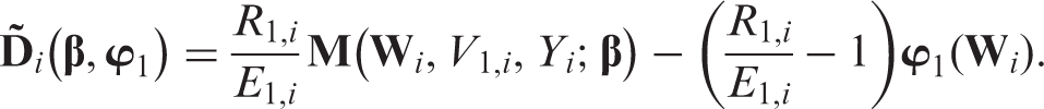
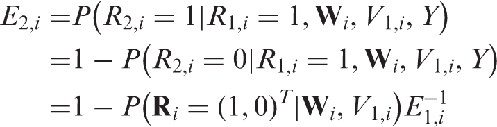
Here $ϕ_{1}$ is a vector of selected functions of the observed components $W_{i}$ . However, the first term in ${\tilde{D}}_{i} (β, ϕ_{1})$ depends on the outcome Y_i which might still be missing in the actual data even if $R_{1, i} = 1$ . To obtain unbiased estimating equations that depend only on the observed data $O_{i}$ , in the second stage of our estimation procedure, we apply the IPW approach to the second artificial missingness model, where $O_{i}^{♦}$ is now the full data and $O_{i}$ is the observed data. Note that in this artificial missingness model, the missing indicator does not equal $R_{2, i}$ . Rather, the missing indicator equals one when the ‘full’ data and the observed data are the same. Since $O_{i} = O_{i}^{♦}$ if $R_{1, i} = 0$ or $R_{1, i} = R_{2, i} = 1$ , we define a new missing indicator

{\tilde{R}}_{i} = (1 - R_{1, i}) + R_{2, i}

with

{\tilde{E}}_{i} \equiv P ({\tilde{R}}_{i} = 1 | O_{i}^{♦}) = (1 - R_{1, i}) + R_{1, i} E_{2, i}

. Thus, our second-stage IPW estimators

{{\hat{β}}_{(ϕ_{1}, ϕ_{2})} : (ϕ_{1}, ϕ_{2})}

are solutions to the estimating equation

\sum_{i = 1}^{n} D_{i} (β, ϕ_{1}, ϕ_{2}) = 0

where

\begin{matrix} D_{i} (β, ϕ_{1}, ϕ_{2}) = \frac{{\tilde{R}}_{i}}{{\tilde{E}}_{i}} {\tilde{D}}_{i} (β, ϕ_{1}) - (\frac{{\tilde{R}}_{i}}{{\tilde{E}}_{i}} - 1) ϕ_{2} (W_{i}, R_{1, i}, R_{1, i} V_{1, i}) \\ = \frac{{\tilde{R}}_{i}}{{\tilde{E}}_{i}} \frac{R_{1, i}}{E_{1, i}} M (W_{i}, V_{1, i}, Y_{i}; β) - \frac{{\tilde{R}}_{i}}{{\tilde{E}}_{i}} (\frac{R_{1, i}}{E_{1, i}} - 1) ϕ_{1} (W_{i}) \\ - (\frac{{\tilde{R}}_{i}}{{\tilde{E}}_{i}} - 1) ϕ_{2} (W_{i}, R_{1, i}, R_{1, i} V_{1, i}) . \end{matrix}

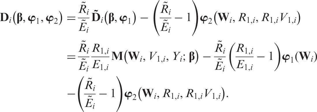
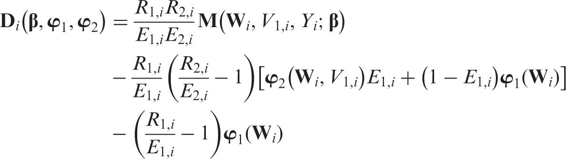
By definition, $\frac{{\tilde{R}}_{i}}{{\tilde{E}}_{i}} \frac{R_{1, i}}{E_{1, i}} = \frac{R_{1, i} R_{2, i}}{E_{1, i} E_{2, i}}$ and $\frac{{\tilde{R}}_{i}}{{\tilde{E}}_{i}} = (1 - R_{1, i}) + R_{1, i} \frac{R_{2, i}}{E_{2, i}}$ . Thus, $({\tilde{R}}_{i} {\tilde{E}}_{i}^{- 1} - 1) ϕ_{2} (W_{i}, R_{1, i}, R_{1, i} V_{1, i}) = R_{1, i} (R_{2, i} E_{2, i}^{- 1} - 1) ϕ_{2} (W_{i}, R_{1, i} = 1, V_{1, i})$ . For simplicity, we denote $ϕ_{2} (W_{i}, R_{1, i} = 1, V_{1, i})$ as $ϕ_{2} (W_{i}, V_{1, i})$ . After some algebra, one has

\begin{matrix} D_{i} (β, ϕ_{1}, ϕ_{2}) = \frac{R_{1, i} R_{2, i}}{E_{1, i} E_{2, i}} M (W_{i}, V_{1, i}, Y_{i}; β) \\ - \frac{R_{1, i}}{E_{1, i}} (\frac{R_{2, i}}{E_{2, i}} - 1) [ϕ_{2} (W_{i}, V_{1, i}) E_{1, i} + (1 - E_{1, i}) ϕ_{1} (W_{i})] \\ - (\frac{R_{1, i}}{E_{1, i}} - 1) ϕ_{1} (W_{i}) \end{matrix}

(5)

Under regularity conditions, it can be proved that ${\hat{β}}_{(ϕ_{1}, ϕ_{2})}$ is a CAN estimator of $β^{*}$ .²¹ Let $ϕ_{1}^{♦} (W_{i}) \equiv ϕ_{1} (W_{i})$ and $ϕ_{2}^{♦} (W_{i}, V_{1, i}) \equiv ϕ_{2} (W_{i}, V_{1, i}) E_{1, i} + (1 - E_{1, i}) ϕ_{1} (W_{i})$ . We can rewrite $D_{i} (β, ϕ_{1}, ϕ_{2})$ as

\frac{R_{1, i} R_{2, i}}{E_{1, i} E_{2, i}} M (W_{i}, V_{1, i}, Y_{i}; β) - \frac{R_{1, i}}{E_{1, i}} (\frac{R_{2, i}}{E_{2, i}} - 1) ϕ_{2}^{♦} (W_{i}, V_{1, i}) - (\frac{R_{1, i}}{E_{1, i}} - 1) ϕ_{1}^{♦} (W_{i}) .

To maximise efficiency under MAR, we select $ϕ_{2}^{♦} (W_{i}, V_{1, i})$ to be $E [M (W_{i}, V_{1, i}, Y_{i}; β) | R_{i} = 1, W_{i}, V_{1, i}]$ and $ϕ_{1}^{♦} (W_{i})$ to be $E [ϕ_{2}^{♦} (W_{i}, V_{1, i}) | R_{1, i} = 1, W_{i}]$ . See Robins, Rotnitzky, and others for further discussions of efficiency.^{5,6,20–22,24,25,40}

Next we consider how to estimate $E_{1, i}$ and $E_{2, i}$ under MAR and MNAR mechanisms, respectively.

5.1 Missing at random

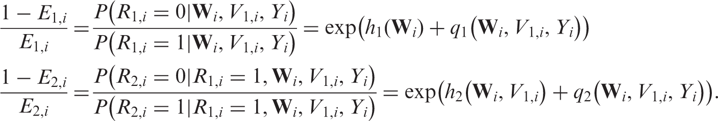
If MAR holds, then for $r = (r_{1}, r_{2})^{T} \in {1, 0, (1, 0)^{T}}$ ,

π_{i} (W_{i}, V_{1, i}, Y, r) = P (R_{i} = r | W_{i}, V_{1, i}, Y_{i}) = P (R_{i} = r | W_{i}, r_{1} V_{1, i}, r_{2} Y_{i}) .

Thus, $E_{1, i} = 1 - P (R_{i} = 0 | W_{i}) = P (R_{1, i} = 1 | W_{i})$ is a function of $W_{i}$ only, whereas

\begin{matrix} E_{2, i} = P (R_{2, i} = 1 | R_{1, i} = 1, W_{i}, V_{1, i}, Y) \\ = 1 - P (R_{2, i} = 0 | R_{1, i} = 1, W_{i}, V_{1, i}, Y) \\ = 1 - P (R_{i} = (1, 0)^{T} | W_{i}, V_{1, i}) E_{1, i}^{- 1} \end{matrix}

depends on

(W_{i}, V_{1, i})

. That is,

E_{2, i} = P (R_{2, i} = 1 | R_{1, i} = 1, W_{i}, V_{1, i})

. Therefore,

E_{1, i}

can be estimated using the observed data

{(R_{1, i}, W_{i}) : i = 1, \dots, n}

by regressing

R_{1, i}

W_{i}

using either a parametric working model or data-adaptive non-parametric techniques. Similarly,

E_{2, i}

can be estimated using the observed data

{(R_{2, i}, W_{i}, V_{1, i}) : i \in {1, \dots, n} and R_{1, i} = 1}

by regressing

R_{2, i}

(W_{i}, V_{1, i})

among those with

R_{1, i} = 1

5.2 Missing not at random

When the missing data process depends on possibly unobserved data and the full data model is non-parametric, we must impose additional assumptions to make the parameters of interest identifiable. We extend the sensitivity analysis approach for the uniform missing pattern and assume that

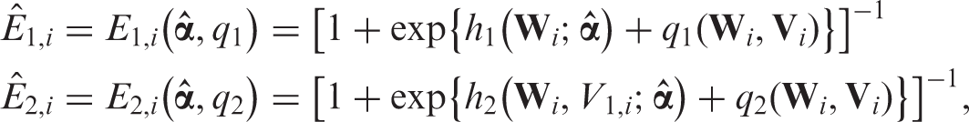
\begin{matrix} \frac{1 - E_{1, i}}{E_{1, i}} = \frac{P (R_{1, i} = 0 | W_{i}, V_{1, i}, Y_{i})}{P (R_{1, i} = 1 | W_{i}, V_{1, i}, Y_{i})} = \exp (h_{1} (W_{i}) + q_{1} (W_{i}, V_{1, i}, Y_{i})) \\ \frac{1 - E_{2, i}}{E_{2, i}} = \frac{P (R_{2, i} = 0 | R_{1, i} = 1, W_{i}, V_{1, i}, Y_{i})}{P (R_{2, i} = 1 | R_{1, i} = 1, W_{i}, V_{1, i}, Y_{i})} = \exp (h_{2} (W_{i}, V_{1, i}) + q_{2} (W_{i}, V_{1, i}, Y_{i})) . \end{matrix}

Here, $q_{1} (W_{i}, V_{1, i}, Y_{i})$ and $q_{2} (W_{i}, V_{1, i}, Y_{i})$ are investigator-specified selection bias functions. To estimate $h_{1} (W_{i})$ and $h_{2} (W_{i}, V_{1, i})$ , we impose parametric working models $h_{1} (W_{i}; α)$ and $h_{2} (W_{i}, V_{1, i}; α)$ , and obtain the estimated parameter $\hat{α}$ by solving the unbiased estimating equation $\sum_{i = 1}^{n} A_{i} (ψ) = 0$ where

A_{i} (ψ) = \sum_{r \in {0, (1, 0)^{T}}} {I (R_{i} = r) - \frac{I (R_{i} = 1)}{π_{i} (W_{i}, V_{i}, 1; \hat{α}, q_{1}, q_{2})} π_{i} (W_{i}, V_{i}, r; \hat{α}, q_{1}, q_{2})} ψ_{r} (W_{i}, r (V_{1, i}, Y_{i})^{T})

Here

\begin{matrix} {\hat{E}}_{1, i} = E_{1, i} (\hat{α}, q_{1}) = [1 + \exp {h_{1} (W_{i}; \hat{α}) + q_{1} (W_{i}, V_{i})}]^{- 1} \\ {\hat{E}}_{2, i} = E_{2, i} (\hat{α}, q_{2}) = [1 + \exp {h_{2} (W_{i}, V_{1, i}; \hat{α}) + q_{2} (W_{i}, V_{i})}]^{- 1}, \end{matrix}

π_{i} (W_{i}, V_{i}, 1; \hat{α}, q_{1}, q_{2}) = {\hat{E}}_{1, i} {\hat{E}}_{2, i}

π_{i} (W_{i}, V_{i}, (1, 0)^{T}; \hat{α}, q_{1}, q_{2}) = {\hat{E}}_{1, i} (1 - {\hat{E}}_{2, i})

, and

π_{i} (W_{i}, V_{i}, 0; \hat{α}, q_{1}, q_{2}) = 1 - {\hat{E}}_{1, i}

. Moreover,

ψ_{r} (W_{i}, r (V_{1, i}, Y_{i})^{T})

is a vector of functions of the variables that are observed when

R_{i} = r

5.3 General monotone results

The results we introduced above for example 2 can be extended to multiple-occasion monotone missing data models. In such models, $V_{i}$ consists $q \geq 2$ elements and $R_{i}$ indicates the corresponding vector of missing indicators. If the sth component ( $1 \leq s \leq q$ ) $V_{s, i}$ is missing ( $R_{s, i} = 0$ ), all subsequent components of $V_{i}$ are missing ( $R_{t, i} = 0$ for any $s < t \leq q$ ). Let $r_{s} \equiv (1_{q - s}^{T}, 0_{s}^{T})^{T}$ indicate a q-dimensional vector with the first $q - s$ elements being 1 and the remaining s elements being 0 (i.e. the first $q - s$ elements of $V_{i}$ are observed while the remaining s elements are missing). The class of IPW estimators $\hat{β}$ is constructed based on the estimating equations $\sum_{i = 1}^{n} D_{i} (β, ϕ_{1}, \dots, ϕ_{q})$ where

\begin{matrix} D_{i} (β, ϕ_{1}, \dots, ϕ_{q}) = \frac{I (R_{i} = 1)}{π_{i} (W_{i}, V_{i}, 1)} M (W_{i}, V_{i}; β) \\ + \sum_{s = 1}^{q} {I (R_{i} = r_{s}) - \frac{I (R_{i} = 1)}{π_{i} (W_{i}, V_{i}, 1)} π_{i} (W_{i}, V_{i}, r_{s})} ϕ_{s} (W_{i}, V_{(r_{s}), i}), \end{matrix}

where

ϕ_{s} (W_{i}, V_{(r_{s}), i})

is a vector of selected functions of the variables

W_{i}

and

(V_{1, i}, \dots, V_{q - s, i})^{T}

, which are observed when

R_{i} = r_{s}

. For any

1 \leq s \leq q

, let

E_{s, i} \equiv P (R_{s, i} = 1 | R_{s - 1, i} = 1, W_{i}, V_{i})

denote subject i’s conditional probability of observing the sth element

V_{s, i}

given the full data

(W_{i}, V_{i})

and the event that all previous elements

(V_{1, i}, \dots, V_{s - 1, i})

are observed. Due to monotone missingness,

π_{i} (W_{i}, V_{i}, r_{s}) = Π_{t = 1}^{q - s} E_{t, i} (1 - E_{q - s + 1, i})

Under MAR, $E_{s, i}$ depends on $(W_{i}, V_{1, i}, \dots, V_{s - 1, i})$ only, i.e. $P (R_{s, i} = 1 | R_{s - 1, i} = 1, W_{i}, V_{i}) = P (R_{s, i} = 1 | R_{s - 1, i} = 1, W_{i}, V_{1, i}, \dots, V_{s - 1, i})$ . Then $E_{s, i}$ can be estimated from the observed data ${R_{s, i}, W_{i}, V_{1, i}, \dots, V_{s - 1, i} : i = 1, \dots,, n and R_{s - 1, i} = 1}$ by regressing $R_{s, i}$ on $(W_{i}, V_{1, i}, \dots, V_{s - 1, i})$ among those with $R_{s - 1, i} = 1$ .

The estimation of the missing data process under MNAR is much more complicated. As before, selection bias functions need to be specified for the ‘odds’ of having missing data. Specifically, for any $1 \leq s \leq q$ ,

\begin{matrix} \frac{1 - E_{s, i}}{E_{s, i}} = \frac{P (R_{s, i} = 0 | R_{s - 1, i} = 1, W_{i}, V_{i})}{P (R_{s, i} = 1 | R_{s - 1, i} = 1, W_{i}, V_{i})} \\ = \exp (h_{s} (W_{i}, V_{1, i}, \dots, V_{s - 1, i}; α) + q_{s} (W_{i}, V_{i})) \end{matrix}

Then $π_{i} (W_{i}, V_{i}, r_{s}; α) = Π_{t = 1}^{q - s} E_{t, i} \times (1 - E_{q - s + 1, i})$ and $π_{i} (W_{i}, V_{i}, 1; α) = Π_{t = 1}^{q} E_{t, i}$ . The estimated $\hat{α}$ solves the estimating equation $\sum_{i = 1}^{n} A_{i} (ψ, α) = 0$ where

A_{i} (ψ, α) = \sum_{s = 1}^{q} {I (R_{i} = r_{s}) - \frac{I (R_{i} = 1)}{π_{i} (W_{i}, V_{i}, 1; α)} π_{i} (W_{i}, V_{i}, r_{s}; α)} ψ_{s} (W_{i}, V_{1, i}, \dots, V_{q - s, i}),

and

ψ_{s} (W_{i}, V_{1, i}, \dots, V_{q - s, i})

is a vector of functions of

(W_{i}, V_{1, i}, \dots, V_{q - s, i})

6 Non-monotone missing pattern

In non-monotone missing data models, the q-dimensional vector of missing indicators $R_{i}$ can take $2^{q}$ possible values as each element can be either 0 or 1. For example, when $q = 2$ , $R_{i} = r \in {(0, 0)^{T}, (0, 1)^{T}, (1, 0)^{T}, (1, 1)^{T}}$ . In such models, the estimation of the missing data process is substantially more challenging.

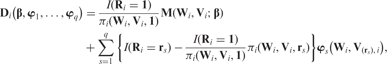
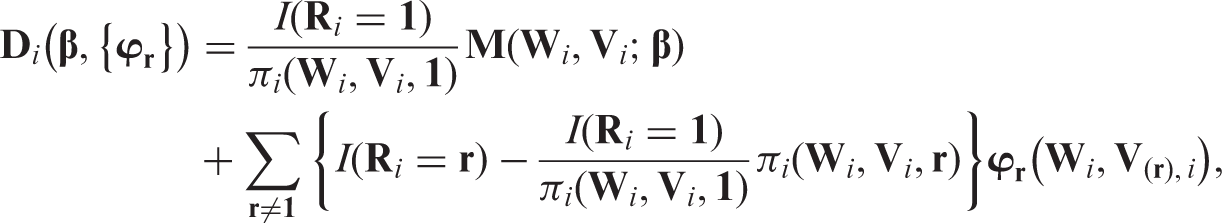
The estimation of the parameter of interest β when the missing probabilities ${π_{i} (W_{i}, V_{i}, r) : r}$ are known is similar to the estimation in monotone missing data models. Specifically, the IPW estimator $\hat{β}$ is obtained by solving the estimating equation $\sum_{i = 1}^{n} D_{i} (β, {ϕ_{r}})$ where

\begin{matrix} D_{i} (β, {ϕ_{r}}) = \frac{I (R_{i} = 1)}{π_{i} (W_{i}, V_{i}, 1)} M (W_{i}, V_{i}; β) \\ + \sum_{r \neq 1} {I (R_{i} = r) - \frac{I (R_{i} = 1)}{π_{i} (W_{i}, V_{i}, 1)} π_{i} (W_{i}, V_{i}, r)} ϕ_{r} (W_{i}, V_{(r), i}), \end{matrix}

and

ϕ_{r} (W_{i}, V_{(r), i})

is a selected

m \times 1

vector of functions of the observed components

(W_{i}, V_{(r), i})

when

R_{i} = r

. Unlike in Section 5.3, r is no longer restricted to

{(1_{q - s}^{T}, 0_{s}^{T})^{T} : 1 \leq s \leq q}

In most applications, $π_{i} (W_{i}, V_{i}, r)$ is unknown and must be estimated from the observed data. Robins and colleagues proposed the randomised monotone missingness (RMM) processes⁴¹ to analyse non-monotone ignorable missing data, and the selection bias permutation missingness (PM) models^42,43 to analyse non-monotone non-ignorable missing data. These approaches are sometimes plausible. However, they are quite complex and computationally intensive. There currently exists no user-friendly software program to facilitate their implementation. These limitations likely contribute to lack of wide adoption. Through introducing the heuristic ideas behind these approaches, we hope to encourage researchers to develop user-friendly software tools for these methods.

We use two motivating examples for MAR and MNAR mechanisms respectively; PM models are best explained in the context of a longitudinal study. In contrast, RMM models do not apply to longitudinal data. Both examples share common notation. The full data is denoted by $L_{i} = {(W_{i}^{T}, V_{1, i}, V_{2, i}, V_{3, i})^{T}, i = 1, \dots, n}$ , and the observed data is denoted by ${O_{i} = (W_{i}^{T}, R_{1, i}, R_{2, i}, R_{3, i}, R_{1, i} V_{1, i}, R_{2, i} V_{2, i}, R_{3, i} V_{3, i})^{T}, i = 1, \dots, n}$ where $R_{i} = (R_{1, i}, R_{2, i}, R_{3, i})^{T}$ is the vector of missing indicators. The parameter of interest $β^{*}$ is the unique solution to $E [M (W, V; β^{*})] = 0$ .

6.1 Missing at random

We consider example 3. Under MAR, for any $r = (r_{1}, r_{2}, r_{3})^{T}$ , $π_{i} (W_{i}, V_{i}, r) = P (R_{i} = r | W_{i}, V_{i}) = P (R_{i} = r | W_{i}, r_{1} V_{1, i}, r_{2} V_{2, i}, r_{3} V_{3, i})$ .

If $(W_{i}, V_{i})$ is discrete with few levels, the estimated missing probabilities ${\hat{π}}_{i} (W_{i}, V_{i}, r)$ can be obtained as the empirical proportions within each covariate level. In practice, we need to impose parametric working models for $π_{i} (W_{i}, V_{i}, r)$ to reduce dimension and borrow information across different covariate levels. To simultaneously satisfy the restrictions imposed by MAR, the inequalities $0 \leq π_{i} (r) \leq 1$ , and the equality $\sum_{r} π_{i} (r) = 1$ , it will be difficult, if not impossible, to directly model ${π_{i} (W_{i}, V_{i}, r) : r}$ .

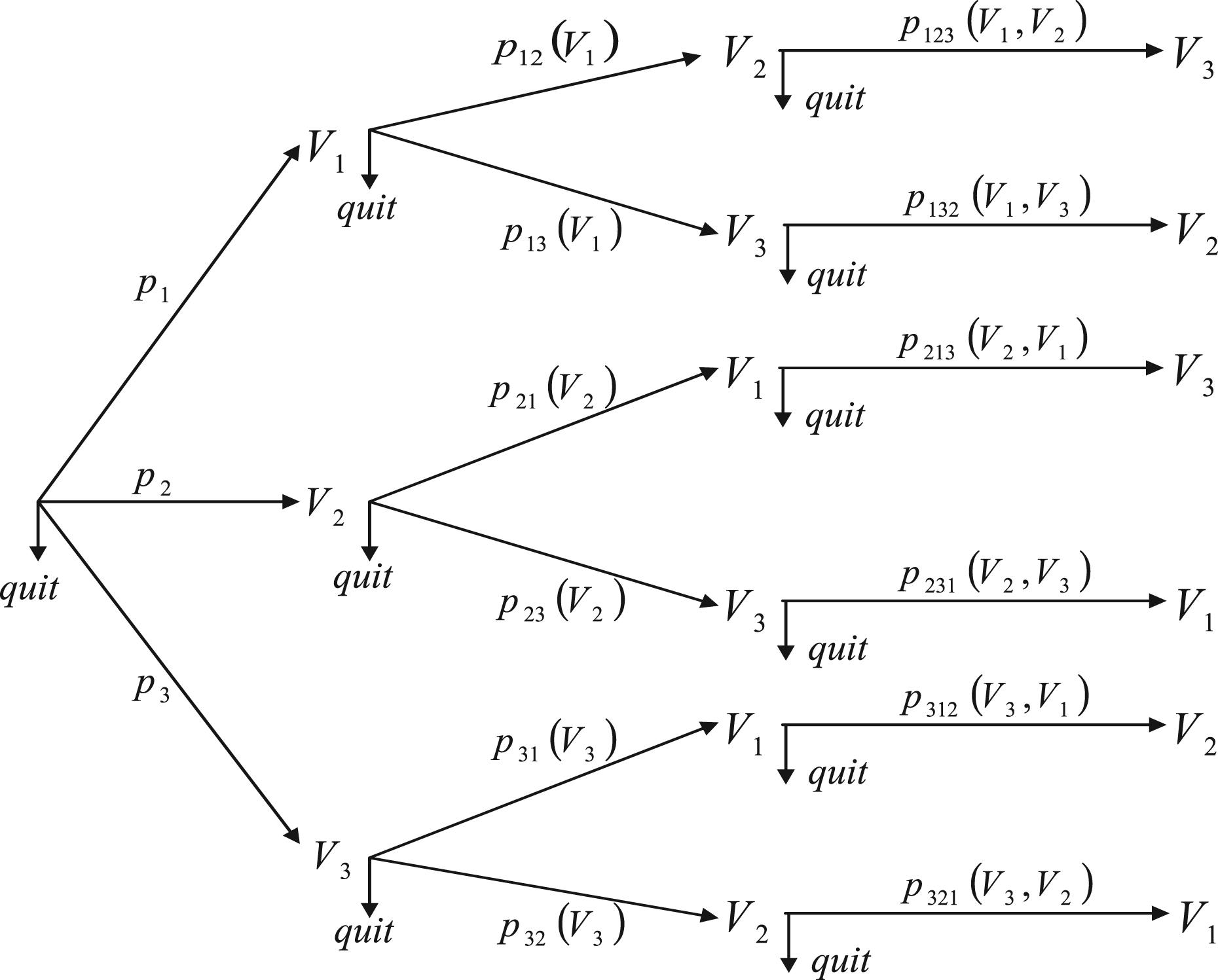
Robins and Gill⁴¹ proposed an algorithm to estimate $π_{i} (W_{i}, V_{i}, r)$ under a sub-model of MAR models, which they referred to as a RMM model. This model is assumed to be generated as follows. For each subject i, $W_{i}$ is observed. Then one of the three elements of $V_{i}$ , $V_{s, i}$ , $1 \leq s \leq 3$ is observed with probability $p_{s} = p_{s} (W_{i})$ , or one quits without observing any element of $V_{i}$ with probability $q = 1 - \sum_{s = 1}^{3} p_{s}$ . If, for example, $V_{1, i}$ is observed, then in a second step, we observe $V_{2, i}$ with a conditional probability $p_{12} (V_{1, i})$ , or observe $V_{3, i}$ with a conditional probability $p_{13} (V_{1, i})$ , or quit with probability $1 - p_{12} (V_{1, i}) - p_{13} (V_{1, i})$ . Note that the conditional probabilities $p_{12} (V_{1, i})$ and $p_{13} (V_{1, i})$ depend both on $W_{i}$ and the value of $V_{1, i}$ observed at the first step. For simplicity, we suppress the dependence on $W_{i}$ when no ambiguity arises. Suppose $V_{2, i}$ is observed at the second step, then in the third step, we observe the third component $V_{3, i}$ with a conditional probability $p_{123} (V_{1, i}, V_{2, i})$ or quit with probability $1 - p_{123} (V_{1, i}, V_{2, i})$ . The following figure is similar to Figure 1 in Robins and Gill⁴¹ to help understanding.

Figure 1.

Missing data process in a RMM process.

An RMM process satisfies MAR. For example, the overall probability of observing $(V_{1, i}, V_{2, i})$ , $π_{i} (r = (1, 1, 0)^{T})$ , equals $p_{1} p_{12} (V_{1, i}) (1 - p_{123} (V_{1, i}, V_{2, i})) + p_{2} p_{21} (V_{2, i}) (1 - p_{213} (V_{2, i}, V_{1, i}))$ , since we either observe $V_{1, i}$ at the first step and then $V_{2, i}$ at the second step and then quit without observing $V_{3, i}$ , or observe $V_{2, i}$ at the first step and then $V_{1, i}$ at the second step and then quit without observing $V_{3, i}$ . This overall probability depends on $(W_{i}, V_{1, i}, V_{2, i})$ which are observed when $R_{i} = (1, 1, 0)^{T}$ . It can be shown that the probabilities sum to 1.

Gill and Robins⁴⁴ showed that there do exist ignorable (i.e. MAR) missing data processes that are not RMM. However, such processes are often unrealistic ‘due to the subtle and precise manner in which the data must be “hidden” to insure that the process is MAR’.

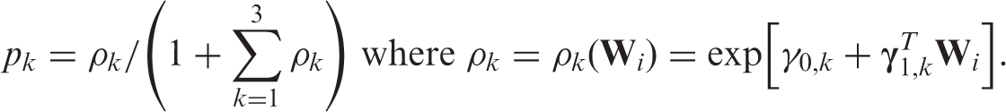
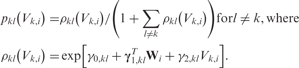
The estimation of $π_{i} (W_{i}, V_{i}, r)$ is non-trivial for RMM processes. To reduce the dimension, the authors considered Markov RMM processes in which the conditional probabilities do not depend on the order in which the variables were observed. For example, $p_{123} (V_{1, i}, V_{2, i}) = p_{213} (V_{1, i}, V_{2, i})$ and will be denoted as $p_{3}^{12} (V_{1, i}, V_{2, i})$ . Parametric working models are imposed for these conditional probabilities. For example, for any $k \in {1, 2, 3}$ , we model the first-step probabilities with a multinomial logistic regression model

p_{k} = ρ_{k} / (1 + \sum_{k = 1}^{3} ρ_{k}) where ρ_{k} = ρ_{k} (W_{i}) = \exp [γ_{0, k} + γ_{1, k}^{T} W_{i}] .

The second-step probabilities are modelled by

\begin{matrix} p_{kl} (V_{k, i}) = ρ_{kl} (V_{k, i}) / (1 + \sum_{l \neq k} ρ_{kl} (V_{k, i})) for l \neq k, where \\ ρ_{kl} (V_{k, i}) = \exp [γ_{0, kl} + γ_{1, kl}^{T} W_{i} + γ_{2, kl} V_{k, i}] . \end{matrix}

Finally, the third-step probabilities are modelled by,

\log it [p_{k}^{{1, 2, 3} \ k} (V_{(- k), i})] = ζ_{0, k} + ζ_{1, k}^{T} W_{i} + ζ_{2, k}^{T} V_{(- k), i}, k \in {1, 2, 3},

where

V_{(- k), i}

indicates the two elements other than

V_{k, i}

(e.g.,

V_{(- 1), i} = (V_{2, i}, V_{3, i})^{T}

). When appropriate, we can further decrease the dimension of the parameter space by assuming, for example,

(γ_{0, k}, γ_{1, k}^{T})

does not depend on k.

The maximum likelihood estimates (MLEs) of the unknown parameters cannot be directly obtained as the order in which variables were observed is missing. For example, there are two paths in the figure above by which $V_{1, i}$ and $V_{2, i}$ could be observed: $V_{1, i} - V_{2, i} - quit$ , or $V_{2, i} - V_{1, i} - quit$ . The authors suggest treating the path information as missing and to obtain the MLE with the Expectation-Maximisation (EM) algorithm. See Ref.⁴¹ for details.

6.2 Missing not at random

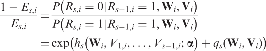
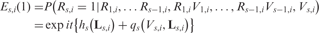
For non-monotone non-ignorable missing data processes, Robins et al.⁴³ propose selection bias PM models. Consider our motivating example 4, a longitudinal study with three BP measurements. In longitudinal studies, the PM order is the reverse of the temporal order. Under a PM model, we assume that the conditional probability of observing $V_{s, i}$ at the sth visit depends (i) on the observed components from previous visits (i.e. $L_{s, i} \equiv (W_{i}, R_{1, i}, \dots R_{s - 1, i}, R_{1, i} V_{1, i}, \dots, R_{s - 1, i} V_{s - 1, i})$ ) but not on the unobserved components of $(V_{1, i}, \dots, V_{s - 1, i})$ ; (ii) on the value of $V_{s, i}$ through a specified selection bias function; and (iii) on both observed and unobserved components in future visits ( $(V_{s + 1, i}, \dots, V_{q, i})$ ). In our motivating example 4, we consider a simplified PM model in which the conditional probability of observing $V_{s, i}$ does not depend on any future data. Thus, $π_{i} (W_{i}, V_{i}, r) = P (R_{i} = r | W_{i}, V_{i})$ is $Π_{s = 1}^{3} E_{s, i} (r_{s})$ , where $E_{s, i} (r_{s}) \equiv P (R_{s, i} = r_{s} | R_{1, i} = r_{1}, \dots, R_{s - 1, i} = r_{s - 1}, W_{i}, V_{i})$ satisfies

\begin{matrix} E_{s, i} (1) = P (R_{s, i} = 1 | R_{1, i}, \dots R_{s - 1, i}, R_{1, i} V_{1, i}, \dots, R_{s - 1, i} V_{s - 1, i}, V_{s, i}) \\ = \exp it {h_{s} (L_{s, i}) + q_{s} (V_{s, i}, L_{s, i})} \end{matrix}

(6)

Here $q_{s} (V_{s, i}, L_{s, i})$ is an investigator specified selection bias function and $h_{s} (L_{s, i})$ is an unrestricted function to be estimated. By Equation (6), the conditional probability $E_{s, i} (r_{s})$ depends on the possibly unobserved value of $V_{s, i}$ through $q_{s} (V_{s, i}, L_{s, i})$ .

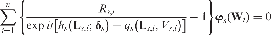
In most applications, we impose parametric working models $h_{s} (L_{s, i}; δ_{s})$ for $h_{s} (L_{s, i})$ to overcome the curse of dimensionality. The parameter $δ_{s}$ can be estimated by solving

\sum_{i = 1}^{n} {\frac{R_{s, i}}{\exp it [h_{s} (L_{s, i}; δ_{s}) + q_{s} (L_{s, i}, V_{s, i})]} - 1} ϕ_{s} (W_{i}) = 0

(7)

where

ϕ_{s} (W_{i})

is a vector of selected known functions of

W_{i}

and has the same dimension as

δ_{s}

. See Vansteelandt et al.³⁰ for an extension of this approach to estimate the mean vector of repeated outcomes in a non-ignorable, non-monotone missing data model.

Although a subject’s decision to miss the sth visit cannot directly depend on future data. But R_s, the indicator variable indicating whether V_s was observed, might be statistically associated with future data, when some factors that affect the decision are not recorded in $(L_{s}, V_{s})$ but are associated with $(V_{s + 1}, \dots,, V_{q})$ . See Robins et al.⁴³ for further discussions.

7 Discussion

We have introduced the IPW approaches in a wide range of settings with different missing data patterns and mechanisms. These weighting approaches share the same basic idea. However, different strategies are needed to estimate the missing probabilities depending on the missing data pattern and mechanism. Our goal in this review article was to provide a conceptual overview of existing weighting approaches.

Our review began with a simple uniform missing data model; for each subject i, either the entire vector $V_{i}$ is observed or it is completely missing. We then discussed monotone missing data patterns. We show these models can be decomposed into multiple ‘artificial’ uniform missing data models and estimators are obtained by applying weighting approaches for uniform missing data models in a nested fashion. In Section 6, we discussed non-monotone missing patterns and notice that the estimation of the missingness probabilities is substantially more challenging and complex. We then introduced the RMM processes for non-monotone MAR data and the selection bias PM approach for non-monotone MNAR data. User-friendly software programs need to be developed to make these methods useful for practice.

We considered both MAR and MNAR mechanisms. IPW estimators for MNAR are natural extensions of IPW estimators for MAR in which selection bias functions quantify the residual association of the missing probabilities and unobserved data conditional on observed data. The MAR assumption cannot be empirically tested when the model of the full data is non-parametric. Subject matter expertise and prior information are typically required to judge its plausibility. In uniform and monotone missing patterns, MAR sometimes is reasonable if data on a large set of variables are collected. The MAR assumption is less likely to hold with non-monotone missingness.³⁰ Unless strong prior information is available, we recommend analysts consider the possibility that the missingness mechanism is non-ignorable and conduct a sensitivity analysis.

References

Little

Rubin

. Statistical analysis with missing data , New York: John Wiley & Sons, 1987.

Raghunathan

. What do we do with missing data? Some options for analysis of incomplete data. Ann Rev Public Health 2004; 25: 99–117.

Rubin

. Inference and missing data (with discussion). Biometrika 1976; 63: 581–592.

Horvitz

Thompson

. A generalization of sampling without replacement from a finite universe. J Am Stat Assoc 1952; 47: 663–685.

Robins

Rotnitzky

Zhao

. Estimation of regression coefficients when some regressors are not always observed. J Am Stat Assoc 1994; 89: 846–866.

Robins

Rotnitzky

Zhao

. Analysis of semiparametric regression models for repeated outcomes in the presence of missing data. J Am Stat Assoc 1995; 90: 106–121.

Robins

Hernan

Brumback

. Marginal structural models and causal inference in epidemiology. Epidemiology 2000; 11: 550–560.

Hernan

Brumback

Robins

. Marginal structural models to estimate the causal effect of Zidovudine on the survival of HIV-positive men. Epidemiology 2000; 11: 561–570.

Horton

Laird

. Maximum likelihood analysis of generalized linear models with missing covariates. Stat Methods Med Res 1999; 8: 37–50.

10.

Ibrahim

Chen

Lipsitz

Herring

. Missing-data methods for generalized linear models: a comparative review. J Am Stat Assoc 2005; 100: 332–346.

11.

Ibrahim

Molenberghs

. Missing data methods in longitudinal studies: a review. Test 2009; 18: 1–43.

12.

Ibrahim

Chen

. Power prior distributions for regression models. Stat Sci 2000; 15: 46–60.

13.

Chen

Ibrahim

Lipsitz

. Bayesian methods for missing covariates in cure rate models. Lifetime Data Anal 2002; 8: 117–146.

14.

Ibrahim

Chen

Lipsitz

. Bayesian methods for generalized linear models with covariates missing at random. Can J Stat 2002; 30: 55–78.

15.

Harel

Zhou

. Multiple imputation: review of theory, implementation and software. Stat Med 2007; 26: 3057–3077.

16.

Rubin

. Multiple imputation for nonresponse in surveys , New York: Wiley, 1987.

17.

Schafer

. Multiple imputation: a primer. Stat Methods Med Res 1999; 8: 3–15.

18.

Tsiatis

. Semiparametric theory and missing data , New York: Springer, 2006.

19.

van der Laan

Robins

. Unified methods for censored longitudinal data and causality , New York: Springer, 2003.

20.

Robins

Rotnitzky

. Semiparametric efficiency in multivariate regression-models with missing data. J Am Stat Assoc 1995; 90: 122–129.

21.

Rotnitzky

Robins

Scharfstein

. Semiparametric regression for repeated outcomes with nonignorable nonresponse. J Am Stat Assoc 1998; 93: 1321–1339.

22.

Robins

Rotnitzky

Zhao

. Analysis of semiparametric regression-models for repeated outcomes in the presence of missing data. J Am Stat Assoc 1995; 90: 106–121.

23.

Rotnitzky

Robins

. Semiparametric regression estimation in the presence of dependent censoring. Biometrika 1995; 82: 805–820.

24.

Rotnitzky

Robins

. Semiparametric estimation of models for means and covariances in the presence of missing data. Scand J Stat 1995; 22: 323–333.

25.

Rotnitzky

Holcroft

Robins

. Efficiency comparisons in multivariate multiple regression with missing outcomes. J Multivariate Anal 1997; 61: 102–128.

26.

Bickel

Klaassen

Ritov

Wellner

. Efficient and adaptive estimation for semiparametric models , New York: Springer Verlag, 1998.

27.

Scharfstein

Rotnitzky

Robins

. Adjusting for nonignorable drop-out using semiparametric nonresponse models. J Am Stat Assoc 1999; 94: 1096–1120.

28.

Scharfstein

Rotnitzky

Robins

. Adjusting for nonignorable drop-out using semiparametric nonresponse models – Rejoinder. J Am Stat Assoc 1999; 94: 1135–1146.

29.

Robins

Rotnitzky

. Inference for semiparametric models: some questions and an answer – Comments. Stat Sin 2001; 11: 920–936.

30.

Vansteelandt

Rotnitzky

Robins

. Estimation of regression models for the mean of repeated outcomes under nonignorable nonmonotone nonresponse. Biometrika 2007; 94: 841–860.

31.

Breiman

Friedman

Olshen

Stone

. Classification and regression trees , Belmont, CA: Wadsworth International Group, 1984.

32.

Friedman

Hastie

Tibshirani

. Additive logistic regression: a statistical view of boosting. Ann Stat 2000; 28: 337–374.

33.

Friedman

Hastie

Tibshirani

. Additive logistic regression: a statistical view of boosting – Rejoinder. Ann Stat 2000; 28: 400–407.

34.

Breiman

. Random forests. Mach Learn 2001; 45: 5–32.

35.

Hastie

Tibshirani

Friedman

. The elements of statistical learning: data mining, inference, and prediction , 2nd ed. New York: Springer, 2009.

36.

Schneeweiss

Rassen

Glynn

Avorn

Mogun

Brookhart

. High-dimensional propensity score adjustment in studies of treatment effects using health care claims data. Epidemiology 2009; 20: 512–522.

37.

Therneau TM and Atkinsoon EJ. An introduction to recursive partitioning using the RPART routines. Technical Report 61, Rochester, MN, Mayo Clinic, Section of Statistics, 1997.

38.

Bang

Robins

. Doubly robust estimation in missing data and causal inference models. Biometrics 2005; 61: 962–972.

39.

Potthoff

Tudor

Pieper

Hasselblad

. Can one assess whether missing data are missing at random in medical studies? Stat. Methods Med Res 2006; 15: 213–234.

40.

Rotnitzky

Robins

. Analysis of semi-parametric regression models with non-ignorable non-response. Stat Med 1997; 16: 81–102.

41.

Robins

Gill

. Non-response models for the analysis of non-monotone ignorable missing data. Stat Med 1997; 16: 39–56.

42.

Robins

. Non-response models for the analysis of non-monotone non-ignorable missing data. Stat Med 1997; 16: 21–37.

43.

Robins

Rotnitzky

Scharfstein

Sensitivity analysis for selection bias and unmeasured confounding in missing data and causal inference models. In: Halloran

Berry

(eds). Statistical models in epidemiology: the environment and clinical trials , New York: Springer-Verlag, 1999, pp. 1–92.

44.

Gill

van der Laan

Robins

Coarsening at random: characterizations, conjectures and counterexamples. In: Lin

(ed.) Proceedings of the first Seattle symposium on biostatistics: survival analysis , New York: Springer Verlag, 1997, pp. 255–294.

On weighting approaches for missing data

Abstract

Keywords

1 Introduction

2 Models and notations

2.1 Missing pattern 1: uniform missing data, i.e. R 1 = " P 427 A 97 56 . . . = " P 427 A 97 56 R q = " P 427 A 97 56 R

2.2 Motivating example 1

2.3 Missing pattern 2: monotone missing data

2.4 Motivating example 2

2.5 Missing pattern 3: non-monotone missing data

2.6 Motivating example 3

2.7 Motivating example 4

3 Why the complete case approach may be biased?

4 Uniform missing pattern

4.1 Missing at random

4.2 Missing not at random

5 Monotone missing pattern

5.1 Missing at random

5.2 Missing not at random

5.3 General monotone results

6 Non-monotone missing pattern

6.1 Missing at random

6.2 Missing not at random

7 Discussion

References

2.1 Missing pattern 1: uniform missing data, i.e. $R_{1} = " P 427 A 97 56 . . . = " P 427 A 97 56 R_{q} = " P 427 A 97 56 R$