
Abstract
The framework of principal stratification provides a way to think about treatment effects conditional on post-randomization variables, such as level of compliance. In particular, the complier average causal effect (CACE) – the effect of the treatment for those individuals who would comply with their treatment assignment under either treatment condition – is often of substantive interest. However, estimation of the CACE is not always straightforward, with a variety of estimation procedures and underlying assumptions, but little advice to help researchers select between methods. In this article, we discuss and examine two methods that rely on very different assumptions to estimate the CACE: a maximum likelihood (‘joint’) method that assumes the ‘exclusion restriction,’ (ER) and a propensity score-based method that relies on ‘principal ignorability.’ We detail the assumptions underlying each approach, and assess each methods' sensitivity to both its own assumptions and those of the other method using both simulated data and a motivating example. We find that the ER-based joint approach appears somewhat less sensitive to its assumptions, and that the performance of both methods is significantly improved when there are strong predictors of compliance. Interestingly, we also find that each method performs particularly well when the assumptions of the other approach are violated. These results highlight the importance of carefully selecting an estimation procedure whose assumptions are likely to be satisfied in practice and of having strong predictors of principal stratum membership.
Keywords
1 Introduction
In randomized experiments, there is often interest not only in the ‘intent-to-treat’ estimate of the effect of randomization, but also in effects conditional on post-randomization variables, such as compliance or dosage levels. The most common way of thinking about these effects is through the framework of principal stratification, 1 which clarifies the need to condition on the potential values of the post-randomization variables, for example compliance behaviour under the treatment condition and under the control condition. While there has been increasing interest in these effects, there has been relatively little investigation of the methods to estimate these effects. This article investigates two approaches for estimating effects conditioned on post-randomization variables: a joint estimation method that uses maximum likelihood (ML) estimation and relies on an assumption called the exclusion restriction (ER), 2 and a propensity score-based approach described in Jo and Stuart 3 that relies on an assumption called principal ignorability (PI). In particular, we detail the assumptions underlying each approach and assess each method's sensitivity to violations of both its own assumptions and those of the other method.
These methods are primarily used in the context of a randomized experiment, where there is interest in estimating treatment effects conditional on a post-randomization variable. The most common contexts are mediation analysis, which aims to investigate the pathways by which treatments may have their effects, 4 and complier average causal effect (CACE) estimation, which aims to estimate the effects of actually taking the treatment, in settings with non-compliance to treatment assignment. 5 Due to additional complications in interpreting mediational effects and linking the results to traditional mediation methods, 6 we focus here on the compliance setting. As is well known, simply conditioning on the observed values of a variable that may be affected by treatment assignment will lead to biased results. The intuition for this in a non-compliance setting is that the people who take the treatment in the treatment group are a self-selected subgroup of the full treatment group; thus, comparing them with the full control group, or with those in both groups who did not take the treatment, will lead to biased results. As formalized by Frangakis and Rubin, 1 the more principled way of controlling for post-randomization variables is to classify individuals into ‘principal strata:’ groups defined by the pair of potential outcomes under treatment and control, for example, the level of treatment received if the individual is in the treatment group and the level of treatment received if the individual is in the control group. In the compliance setting, we can think of these principal strata as defining ‘compliance types,’ as detailed further below. Most work has been in the context of binary post-randomization variables, and that is what we consider here; Jin and Rubin 7 consider continuous dosage levels.
Estimation of the CACE is challenging since it is generally impossible to know any individual's principal stratum membership. The estimation methods thus rely on untestable identifying assumptions. The most commonly used estimation procedures include ML methods that jointly model compliance behaviour and the outcome, Bayesian methods that also incorporate prior distributions and propensity score-based approaches. The propensity score-based approaches are particularly useful in settings where it is possible to identify principal stratum membership for individuals in one of the treatment conditions; the propensity scores are then used to predict the principal stratum membership for individuals in the other condition. In this study, we focus on two methods that rely on very different assumptions: one that relies on the ER and is estimated using a joint model and ML, and one that relies on PI and is estimated using propensity score methods. More details on these methods are provided below.
We motivate our investigation using a randomized trial of an intervention to improve the job search process of unemployed individuals. The Job Search Intervention Study (JOBS II) 8 was a randomized evaluation of a job training programme for unemployed individuals. The treatment condition consisted of five training sessions promoting high-quality reemployment and preventing poor mental health. This intervention was compared with a control condition that consisted of a booklet with job search tips. Fifty-five percent of individuals assigned to the intervention attended at least one of the five sessions, which we define as ‘compliance’; this definition was also used in previous analyses of these data.2,3,9 Interest in the evaluation is in the effect of treatment assignment – the ‘intent-to-treat’ effect – as well as the effect of actually participating in the training sessions – the CACE.
This article proceeds as follows. We first detail the setting considered and the estimation methods that we examine, with particular emphasis on their assumptions, in Section 2. Section 3 then uses simulated data to compare the performance of the approaches, and Section 4 examines the implications for the JOBS II evaluation. Finally, Section 5 provides discussion and conclusions.
2 Setting and estimation methods considered
Using notation from Jo and Stuart, 3 we consider settings where individuals have been randomly assigned to treatment, Z i = 1, or control, Z i = 0. However, not all individuals receive the treatment to which they are assigned. The treatment received is denoted by S, with S i = 1 for individuals who received the treatment and S i = 0 for individuals who did not. Let S i (0) be the treatment received by individual i when in the control condition and S i (1) the treatment received when in the treatment group. We assume that individuals in the control condition cannot access the treatment, and thus S i (0) = 0 for all i, although extensions of the methods could be used when there is non-compliance in both directions.
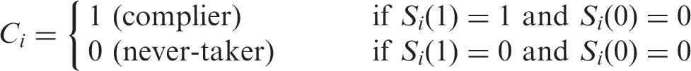
In this setting with binary Z and S, there are two compliance types – two ‘principal strata,’ defined by compliance behaviour under the treatment condition. We denote principal strata membership by C, and have two strata, labelled by Angrist et al.
5
as ‘compliers’ (C
i
= 1) and ‘never-takers’ (C
i
= 0). In particular, compliers will ‘comply’ and take the treatment when it is offered, while never-takers will never take the treatment, even when offered. Throughout the paper we will use the terms ‘never-taker’ and ‘non-complier’ interchangeably. These strata can be more precisely defined as:
As in Jo and Stuart,
3
given these two strata, we consider an outcome Y, which is a function of treatment assignment (Z), compliance type (C) and a single covariate (X):

With the predictor X, using logistic regression, the proportion of compliers can be expressed by π
i
, with P(C
i
= 1|X
i
) = π
i
and P(C
i
= 0|X
i
) = 1 − π
i
, and

The two methods described below will both rely on two assumptions commonly invoked for estimating treatment effects:
Ignorable treatment assignment: that treatment assignment is independent of the potential outcomes given the observed covariates: Z ⊥ [S(0), S(1) Y(0), Y(1)]|X.
10
This assumes that, given the observed covariates, there are no unobserved confounders that would lead to differences across the treatment and control groups in the distributions of the pair of potential outcomes. This assumption is automatically satisfied in randomized experiments. Stable unit treatment value assumption, which has two components: (1) the potential outcomes of each individual are unaffected by the treatment assignments of other individuals (no interference), and (2) there is only one ‘version’ of each treatment condition; i.e., there is one ‘treatment’ given to all treatment group members and one ‘control condition’ given to all control group members – the treatments given to each individual within each treatment condition do not vary across individuals.
11
The additional assumptions that each method requires are detailed below and are the focus of our investigations.
2.1 Estimation methods
We investigate the performance of two methods for estimating the CACE: a method that relies on the ER and is estimated using a joint model of the post-randomization variable (compliance) and the outcome of ultimate interest, and a method that relies on PI that is estimated using propensity score weighting. The following sections detail each of these methods, including their underlying assumptions.
2.1.1 ER joint model
The ER joint estimation procedure simultaneously estimates two models: one of compliance behaviour (principal stratum membership) and one of the outcome, given principal stratum membership. These models are generally estimated using Bayesian or ML methods; we consider ML estimation here. The joint models generally require distributional assumptions as well as assumptions about the relationships between covariates, compliance and outcomes. We consider one of the most common joint estimation procedures, which relies on an explicit assumption about the size of the NACE in order to estimate the CACE. This assumption is the ‘ER’, and assumes that there is no effect of treatment assignment for the never-takers: NACE = γ n = 0. In other words, that if the treatment assignment does not affect the treatment individuals actually receive, then it also will not affect their outcome. The second assumption is distributional, generally an assumption of normally distributed outcomes. With these two identifying assumptions, ML estimation can be done using the expectation-maximization (EM) algorithm. When the ER is assumed, the assumption of normality does not play a primary role in identifying the CACE. Nonetheless, since normality is assumed in the ML–EM method, CACE estimation can be affected by the assumption. How the assumption of normality affects estimation of the CACE has surprisingly not been well investigated, and is one of the key issues that will be examined in this article.
With the ER, the CACE in the two principal strata setting we consider here could be identified using the instrumental variables estimator.5,9,12 The ML–EM estimator is known to be more efficient in estimating the CACE, although the relative performance of the instrumental variable and ML–EM estimators needs further examination.9,13,14 One advantage of the instrumental variables approach is that estimation of the CACE using that approach depends less on parametric assumptions than does the ML method. However, little study has been conducted to compare the two methods in terms of their sensitivity to deviations from the ER and normality assumptions under various situations. It is also possible to estimate a model that assumes PI, similar to the propensity score approaches described below, but using a ML approach to estimation. 3 Given that it relies on similar assumptions as the propensity score approach, and that in preliminary investigations we found that the joint PI model performed less well than the propensity score approach, we do not discuss this model further.
With the ER assumption, all parameters in the model presented in Equation (1) can be identified with little reliance on parametric assumptions. We used a linear model in Equation (1) for convenience, although it is not necessary for identification. In other words, identification comes not from the specific model form but rather from the identifying assumption (i.e., the ER for the joint method and PI for the propensity score weighting method). Model estimation without the ER assumption can be more dependent on parametric assumptions if covariates are not very strong predictors of compliance status. See Jo 2 for more details on the identification strategy in the presence of covariates. We do not detail the ML–EM estimation of CACE under the ER here because this procedure is quite widely known and introduced detail in several places.2,9,13,15,16 Briefly, the unknown compliance status C in the control condition is handled as missing data via the EM algorithm. The E step computes the expected values of the complete-data sufficient statistics given data and current parameter estimates. The M step computes the complete-data ML estimates with the complete-data sufficient statistics replaced by their estimates from the E step.
2.1.2 Principal ignorability propensity score weighting
The second procedure we examine is based on the assumption of PI and is estimated using propensity score methods, which can be used in settings where principal stratum membership is known under one treatment condition. For example, in the primary setting considered, we can identify principal strata membership for some individuals by identifying which treatment group members actually received the treatment:
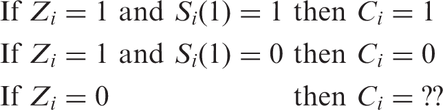
Intuitively, the method works by fitting a model of principal stratum membership among the treatment group members (for whom stratum membership is observed) to predict the (unobserved) stratum membership for the control group members. Propensity scores are traditionally used to estimate treatment effects in non-experimental settings, where the propensity score models receipt of the treatment and can be used to balance the covariates between the individuals who do and do not receive the treatment.10,17 The idea is to make the data look as if it could have arisen from a randomized experiment, at least with respect to the observed covariates. Propensity scores are also becoming increasingly used for estimating other types of causal effects, such as in CACE estimation.18–20 In fact, in the setting considered here, the propensity score model is still modelling treatment receipt, just in the context of an experiment, and that model is estimated using only treatment group members (the model is then applied to the control group to generate predicted probabilities of treatment receipt). While the data could be treated as if it came just from an observational study and the propensity score model could be fit by predicting treatment receipt using the combined treatment and comparison groups, this would not take advantage of the randomization since the randomization indicator could not be included in that model (since it would perfectly predict treatment receipt for the control group members). The approach presented here uses the randomization in being able to apply the compliance model fit using the treatment group to the control group, and because it ensures that there are compliers in the control group.
One of the drawbacks of the joint model approach described earlier is that it requires a joint model of compliance and outcomes, and how the covariates relate to both of those. Some researchers prefer to separate the models; the propensity score approach provides a way to do so. In particular, the propensity score approach consists of two stages: (1) estimating the propensity score model by fitting a logistic regression predicting compliance behaviour in the treatment group, and (2) using that model to predict compliance behaviour under treatment for control group members and then using those predicted probabilities (the propensity scores) in the outcome model. Stage 2 is generally accomplished using matching, weighting or subclassification. 21 Jo and Stuart 3 examined the performance of both propensity score matching and weighting to estimate the CACE, both using a PI assumption; since somewhat better results were found when using weighting we consider only the weighting approach here.
To estimate the CACE using the propensity score approach, we take the following steps:
Estimate a logistic regression of stratum membership, among the treatment group members:
Using the parameter estimates from the model in Step 1, generate the predicted probability of being a complier for each control group member:
Create the weights, w
i
:
Estimate the CACE by fitting regression models of the outcome among the treatment and control group members using the weights created in Step 3.

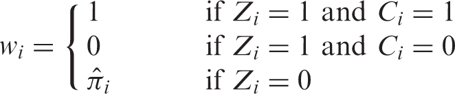
The weights reflect the probability of receiving the treatment, and thus can be thought of as weighting the control group members to look like the compliers. Estimation of the NACE is done using the same procedure, except in Step 3 the treatment group compliers (Z
i
= 1 and C
i
= 1) receive a weight of 0, the treatment group non-compliers (Z
i
= 1 and C
i
= 0) receive a weight of 1, and the control group members receive weights of
The key assumption underlying the propensity score-based approach is ‘PI,’ 3 which says that principal stratum membership is independent of the potential outcomes given the observed covariates: E(C i |X i , Y i (0), Y i (1)) = E(C i |X i ). A way to express the PI assumption in terms of Equation (1) is that α c = α n and λ c = λ n , and it can also be expressed in terms of conditional independence: Y i (0), Y i (1) ⊥ C i |X i . Principal ignorability is related to the ignorability assumption in observational studies, which states that treatment assignment is independent of the potential outcomes, given the observed covariates. In the compliance setting, this assumption implies that we can identify principal stratum membership using only the observed covariates. This is what enables us to find the ‘likely compliers’ in the control group, using the model of compliance behaviour as a function of covariates fit among treatment group members; i.e., it implies that the outcomes of the control group members identified as ‘likely compliers’ actually reflect well what the potential outcomes under control would have been had the treatment group compliers been in the control group instead.
3 Monte carlo simulation study
Unfortunately the ER and PI assumptions are not directly testable, and it is sometimes difficult to fully assess the normality assumption. It is likely that in any real data analysis, any or all these assumptions are violated at least somewhat. A simulation study was done to assess the sensitivity of results to violations of these crucial assumptions, to help researchers better understand the implications of violations of the assumptions for the two primary estimation methods.
3.1 Simulation design
We consider a setting with a single covariate X and principal stratum membership and outcome models following Equations (1) and (2). The covariate X is generated to follow a N(0, 1) distribution. The true treatment probability was 0.5 and the proportion of compliers is also 0.5. We performed 1000 replications, each with a sample size of 500. We compare the performance of the two estimators: the ER joint model and PI propensity score weighting.
Throughout the simulations, we assume a true value for CACE of 0.5 (γ c = 0.5). The relationship between the covariate and the outcome, parameterized by λ c and λ n , is set to be the same across the two strata (λ c = λ n ), so that the difference between α c and α n characterizes the full source of deviation from PI. We allow the strength of the relationship between C and X to vary, expressed as an odds ratio (OR), from 0.1 to 0.5.
We consider three types of violations of the assumptions:
Violations of the ER: If the ER holds, then the NACE (γ
n
) is 0. We consider three scenarios: true NACE=0, true NACE=CACE and true NACE= −1*CACE. In most settings, it is extremely unlikely that the absolute size of the NACE would be more than that of the CACE, and thus we believe these three scenarios safely cover a range of reasonable values for the NACE. Violations of normality: We perform some simulations that meet the normality assumption, with ε
i
∼ N(0, 1) for both compliers and never-takers. In other simulations, we violate this assumption and, for the compliers, instead draw ε from a mixture of two normal distributions that are 3 standard deviations (SD) apart. This yields a symmetric but bimodal distribution for the complier potential outcomes (see Figure 1 for an illustration of this distribution). Violations of PI: As described above, the difference between α
c
and α
n
characterizes the extent to which PI is satisfied. When α
c
= α
n
, PI is satisfied. We also consider two violations of PI, with α
c
= 1 always, and α
c
− α
n
equal to 0.5 or 1.0. (Since the residual variance equals 1, these can be thought of as SD units). Distribution when normality is violated. Note: Density plot of a distribution that is a 50/50 mixture of Normal(0, 1) and Normal(3, 1).
For each simulated dataset, we estimate the CACE using the joint model, which assumes the ER and normality, and the propensity weighting approach, which assumes PI. For both estimators we calculate the bias, the empirical standard error, root mean square error and coverage (nominal level 95%). Note that, in the data generation procedure, we used a bimodal distribution for the complier potential outcomes to create sufficient non-normality. As a result, the total variance exceeds 1 in the non-normal settings, which makes comparisons across simulation settings somewhat difficult. (i.e., some have total variance of 1, and some do not) Given this limitation, readers are encouraged to evaluate the quality of estimation not just in terms of coverage and root mean square error, but also in terms of the bias. For all simulations, the data generation and joint model estimation were done in Mplus
22
and the propensity weighting methods were conducted in R
23
using the MatchIt package.
24

3.2 Simulation results
The Monte Carlo simulation results presented in this study are based on 1000 replications. The bias and root mean square error were calculated for each replication and averaged over 1000 replications. In each replication, model-based standard errors were estimated for each parameter estimate, and then averaged across replications. The Monte Carlo error is on the order of the second or third decimal place and does not affect any of the conclusions.
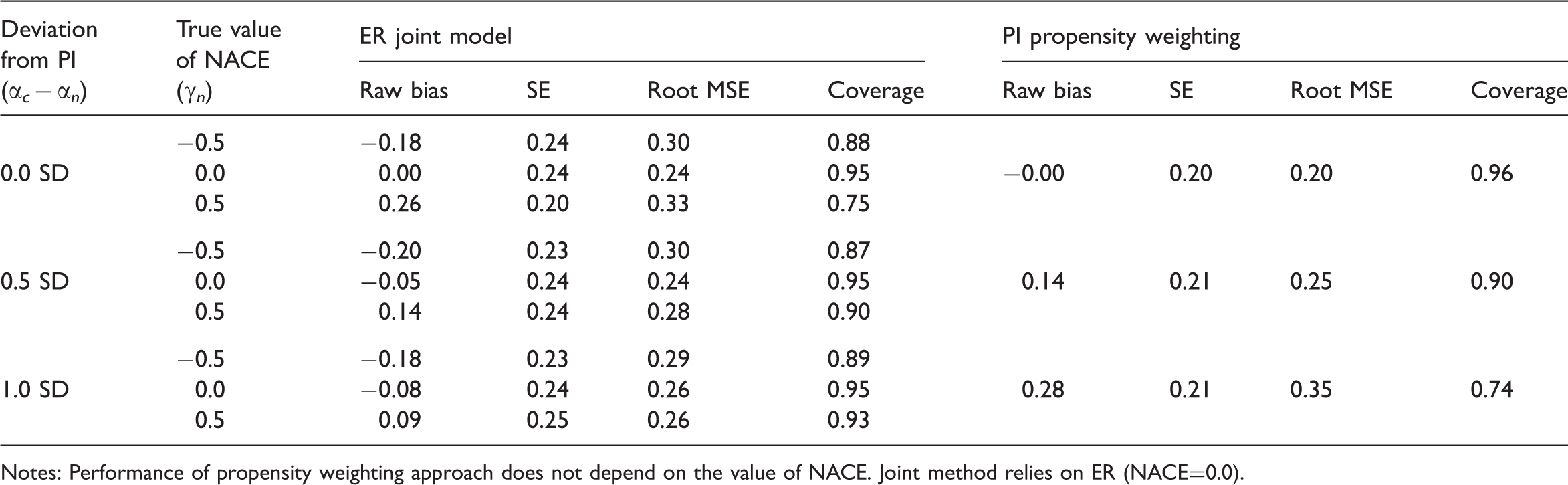
Simulation: CACE estimation when the normality assumption is satisfied and the relationship between X and C is strong (OR=0.1) (true CACE = 0.5)
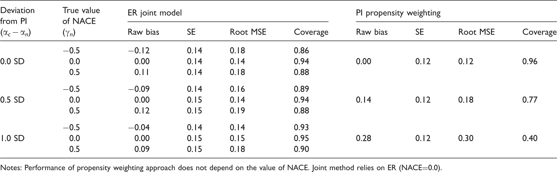
Notes: Performance of propensity weighting approach does not depend on the value of NACE. Joint method relies on ER (NACE=0.0).
Simulation: CACE estimation when the normality assumption is satisfied and the relationship between X and C is weak (OR=0.5) (true CACE = 0.5)

Notes: Performance of propensity weighting approach does not depend on the value of NACE. Joint method relies on ER (NACE=0.0).
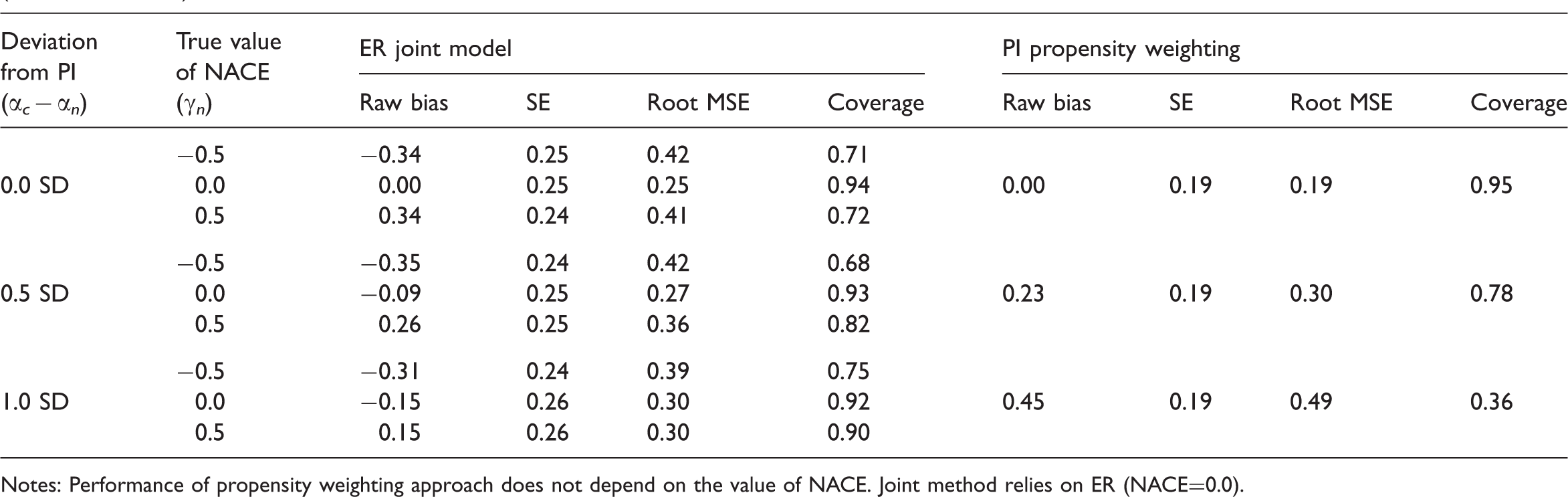
Simulation: CACE estimation when the normality assumption is violated and the relationship between X and C is strong (OR=0.1) (true CACE = 0.5)
Notes: Performance of propensity weighting approach does not depend on the value of NACE. Joint method relies on ER (NACE=0.0).
Simulation: CACE estimation when the normality assumption is violated and the relationship between X and C is weak (OR=0.5) (true CACE = 0.5)
Notes: Performance of propensity weighting approach does not depend on the value of NACE. Joint method relies on ER (NACE=0.0).
In contrast, but also as expected, the performance of each method declines as its assumptions are more strongly violated, especially when the relationship between stratum membership, C, and the covariate, X, is relatively weak (OR=0.5). The propensity score approach is fairly sensitive to violation of PI. When normality is satisfied, even with a strong predictor of stratum membership, the coverage of the weighting approach drops to 77% and then 40% for 0.5 and 1.0 SD violations of PI, respectively (Table 1). When normality is satisfied but such a strong predictor of class membership is not available, the corresponding coverage rates are 48% and an abysmal 3% (Table 2). The performance of the joint model does not get quite as bad as that under the settings we consider, however, even when normality is satisfied, when there is only a weak predictor of stratum membership and the true NACE is 0.5, the root mean square error is as large as 0.46 and coverage as low as 37% (Table 2).
One interesting finding is that each method is not sensitive to the assumptions of the other approach, and in fact each method appears to perform particularly well when the other methods' assumptions are violated. In fact, CACE estimation using the PI propensity weighting approach makes no assumptions about the size of the NACE (since the NACE plays no role when estimating the CACE), and thus the performance of the propensity weighting estimator is exactly the same regardless of the true NACE, and thus regardless of potential violations of the ER (this is why Tables 1–4 do not show separate results for different values of the NACE for the PI propensity weighting approach). Examining the ER joint model's other assumption, normality, we see that the PI propensity weighting approach actually has similar bias but better confidence interval coverage when normality is violated compared to when normality holds (comparing Tables 1 and 3 and Tables 2 and 4). This improved coverage is a result of larger standard errors and thus slightly larger confidence intervals. For example, when there is a weak predictor of compliance status, when normality holds, a setting with a 0.5 SD deviation from PI has only 48% coverage (Table 2), but when normality is not satisfied, that same setting has 78% coverage (Table 4).
The situation is similar, although less extreme, for the ER joint method and violations of PI. Within each table (Tables 1–4), the bias and coverage of the joint method improves somewhat as the violation of PI becomes larger. This likely happens because a violation of PI implies a difference in the potential outcome distributions of the compliers and non-compliers. The joint model, which assumes normality, can use that difference to help identify the compliers and estimate separate parameters for the compliers and non-compliers. In essence, the ER joint model relies on being able to identify two classes from a mixture distribution; if the two components of the mixture distribution are fairly well separated from one another it will be easier to identify them and estimate their parameters. In contrast, the PI propensity weighting method is particularly sensitive to this assumption since it assumes that, conditional on the observed covariates, the outcomes are the same for compliers and non-compliers.
Comparing Tables 1 and 3 as well as 2 and 4, we can see that when normality is violated the standard errors increase not only for the propensity weighting approach but also for the joint method. Therefore, the confidence intervals are widened as well. It seems that based on our simulations, widening of confidence intervals consistently connects to better coverage for the propensity weighting methods but does not always lead to better coverage for the joint method. For example, for the joint method, with PI deviation of 0.5 SD and NACE=0.5, the coverage is 37% in Table 2 (when normality holds) and 82% in Table 4 (when normality does not hold). However, with PI deviation of 1.0 SD and NACE=−0.5, the coverage is 93% in Table 2 (when normality holds) and 75% in Table 4 (when normality does not hold). We suspect that this is because the bias in the joint method can be affected by deviation from normality in many different ways (e.g., bias can cancel out or accumulate), whereas deviation from normality simply widens confidence intervals in the propensity weighting method.
4 Application to JOBS II
JOBS II effects on depression: estimates of key parameters from PI propensity score weighting and ER joint model methods
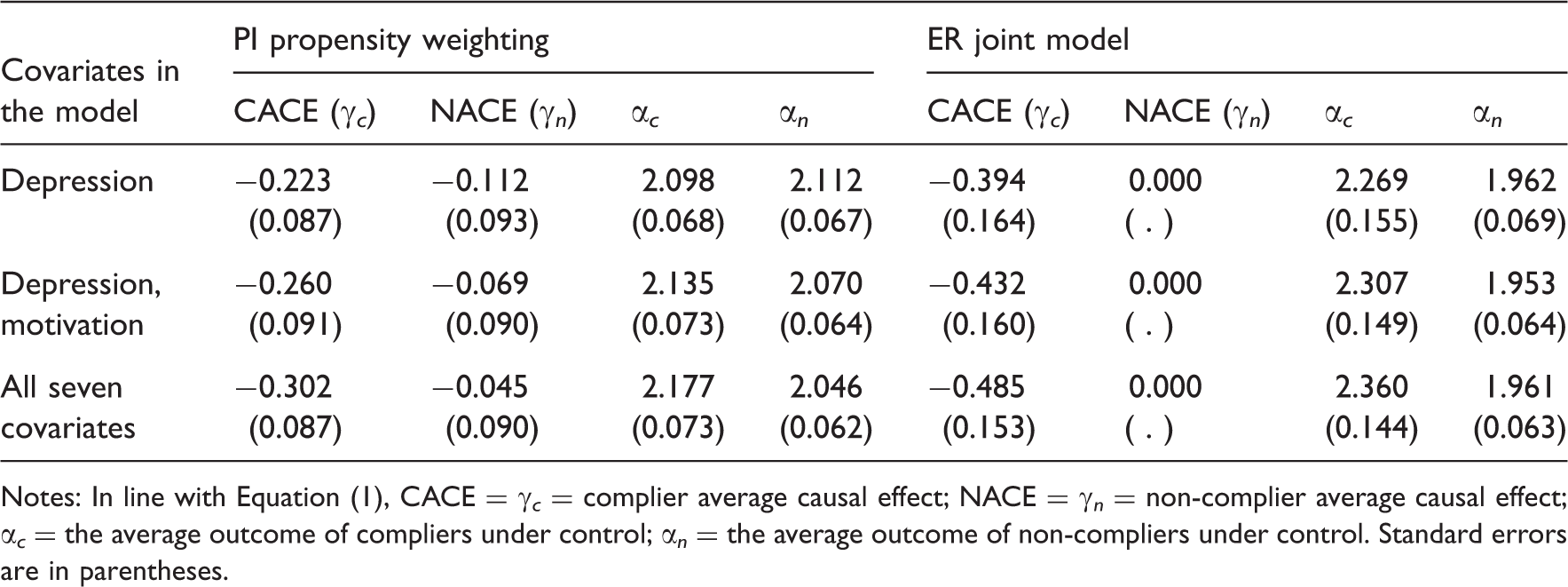
Notes: In line with Equation (1), CACE = γ c = complier average causal effect; NACE = γ n = non-complier average causal effect; α c = the average outcome of compliers under control; α n = the average outcome of non-compliers under control. Standard errors are in parentheses.
We first discuss the plausibility of the ER and PI assumptions in the JOBS II example. In JOBS, where blinding was not used, some deviation from the ER is possible. One possibility is that non-compliers assigned to the treatment condition felt more optimistic about their re-employment possibility. Another possibility is that non-compliers assigned to the treatment condition experienced negative psychological effects (demoralization) of failing to participate in the intervention programme that they were offered. The two scenarios provide opposite bounding information, and we cannot know which scenario is more plausible. However, a substantial deviation from ER is unlikely given that the effect of treatment assignment on non-compliers is mainly psychological. A larger effect on compliers is expected since they are the ones who would receive the intensive JOBS II intervention treatment and the training programme provided critical information and skills necessary for high-quality re-employment and better handling of mental health problems. In line with this scenario, we expect that the absolute size of the NACE is considerably smaller than that of the CACE; Jo and Vinokur 26 label this assumption the ‘average effect restriction’ and use it to construct bounds on the CACE. In terms of PI, we do not expect a dramatic difference in the level of depression between compliers and non-compliers under the control condition. However, we find it more difficult to build scientific assumptions around the PI assumption than around the ER assumption, perhaps in part because it involves assumptions about the differences between compliers and non-compliers, and relatively little is known about why people do (or do not) comply. In addition, as discussed further below, we in fact find some evidence that PI is violated in the JOBS II example, which may make us feel more confident in the results assuming the ER, at least for this particular example.
While the substantive results are similar for the PI propensity weighting and ER joint models, and across the three covariate settings, the results do vary somewhat. In particular, the estimates of the CACE when only depression is included in the model are 70–80% what they are when all seven covariates are included, and the estimates when only depression and motivation are included are approximately 90% what they are when all seven covariates are included. Given that we can never fully assess the validity of the underlying assumptions, a primary benefit of fitting both types of models on the same data is that, given their similar results, we can be more confident in them. However, in addition, as noted in Jo and Stuart, 3 a second benefit of fitting both models in the same data is that one method can inform the validity of the other. In particular, the fact that the NACE estimates when using propensity score matching are close to 0 indicates that the ER may be reasonable, and thus the joint model may be appropriate. The joint model shows that PI might be somewhat violated, in that α c and α n are approximately 0.5 SD apart when all seven covariates are included in the model. However, a severe violation of PI seems unlikely. Given the simulation results above, and the fact that the PI propensity score approach performs best when there are strong predictors of compliance status, we are also more likely to believe the propensity score estimates when all seven covariates are included in the models. The fact that that estimate (−0.302) is closer to the estimates from the joint model approaches also gives us increased confidence that the true CACE in this example is likely on the order of a reduction in depression levels of 0.3 to 0.5 points. In terms of the substantive conclusions, this size CACE (0.3 to 0.5 points) translates to 0.4–0.7 SD (or about one third to one half unit difference in the 5-point scale on which depression was measured), which is not dramatic but is certainly a clinically meaningful effect size, and somewhat higher than the small effect sizes often reported in clinical trials of depression treatment. 27
5 Discussion
Using both simulation and a real-data example, this article has investigated the relative performance of two methods for estimating causal effects within principal strata, a joint model approach that relies on the ER and is estimated using ML, and a propensity score-based approach, which relies on PI and separates the models of principal stratum membership and the outcome into two different stages. We were particularly interested in assessing each methods' sensitivity to its underlying assumptions. The joint model relies on the ER (that NACE=0) and that the outcome values follow a normal distribution. The propensity weighting approach relies on PI: that principal stratum membership is independent of the potential outcomes given the observed covariates.We find that each method is somewhat sensitive to its assumptions, but that the PI propensity score approach in particular performs best when PI is nearly satisfied.
It is particularly interesting to note that the methods perform best under somewhat opposite scenarios. The PI propensity weighting method works better than the ER joint model for no or moderate deviations from PI (0–0.5 SDs), but for larger violations of PI, the joint model outperforms the propensity weighting approach. The ER joint method works very well when PI is strongly violated, and the propensity score approach works quite well when the ER and normality are strongly violated. Unfortunately, the assumptions of the two methods are not directly on the same scale, and thus it is difficult to say definitively how much of a violation of the ER or normality is comparable to a particular deviation from PI. However, we can use Equation (1) to relate the ER and PI assumptions at least somewhat. In particular, since violation of PI is characterized by the difference between α c and α n , we can express it in SD units, as done in Tables 1–4. Similarly, since violation of the ER is characterized by the size of γ n , we can express it too in SD units, as also done in the tables. Thus, by one measure, the violations of PI may seem more ‘extreme’ than the violations of the ER, in that they correspond to 0–1 SD, while the ER violations we consider only span 0–0.5 SD. However, we felt it was unlikely that the NACE would be larger than the CACE in most real data examples, as discussed for the JOBS II example above.
The parametric ER joint estimation method provides a parsimonious one-step analysis, which is convenient especially in the presence of multiple covariates. Much attention has been given to sensitivity of the resulting principal causal effect estimates to violation of the identifying assumptions such as the ER. Relatively little attention has been given to sensitivity of the method to violation of parametric assumptions such as normality. We generally avoid identifying causal effects directly relying on parametric assumptions. However, even in that case, causal effect estimates can be sensitive to violation of these assumptions. Our simulation studies showed that the joint estimation method can be sensitive to violation of normality, in particular when severe violation of normality is accompanied by violation of the ER. When the ER, the key identifying assumption, holds, the joint estimation method is quite insensitive to violation of normality. This is an interesting and important issue that needs to be considered when parametric joint estimation methods are employed. Our simulation results showed that the PI propensity score weighting method is generally less dependent on parametric assumptions. The propensity score method thus adds a valuable option for analysis of sensitivity to the violation of normality. An additional consideration, though, is that in cases where the treatment has no effect at all (CACE=NACE=0), the ER is met and the joint estimation approach is likely to perform very well (assuming non-severe deviations from normality), whereas the PI propensity score approach is not guaranteed to perform well in this case.
This study highlights the need to carefully consider the assumptions underlying different methods and to choose the method that is most suitable for the study at hand. Applied researchers may simply see two methods that both estimate the same quantity, the CACE, and may pick one based on familiarity or ease of implementation. However, it is crucial to target the method to the data and use the method whose assumptions are most likely to be satisfied. It is important to acknowledge that different model assumptions may be preferred in different situations and that instead of pursuing a general conclusion that applies to every occasion (i.e., one assumption always works better than the other), it may make more sense to develop recommendations that take substantive information into account. For example, in two-arm randomized trials with a single active treatment arm (especially with blinding) such as JOBS II, the ER is unlikely to be severely violated in the context of CACE estimation. However, the same assumption may not be as plausible or applicable in trials where multiple active treatments are compared.
This study thus also highlights the importance of developing methods, perhaps through auxiliary studies, for assessing the validity of assumptions, an area that has received relatively little attention in the statistical literature. In settings such as this, where multiple methods can be used to estimate the same quantity, applied researchers need more guidance on how to select the most appropriate approach or to jointly consider results from multiple approaches. Various methods have been developed to assess the validity of assumptions (this is a very wide area of research in causal inference, which includes sensitivity analysis and bounding), although practical methods that are likely to be routinely used are still in need of development. In this article, we intended to promote the use of multiple methods that rely on considerably different identifying assumptions and estimation methods. We acknowledge that this is not a complete solution to sensitivity analysis, but we believethat this will at least promote awareness of the importance of sensitivity analysis and encourage researchers to routinely practice sensitivity analyses starting with relatively accessible methods. As one example, comparing divergences from various model assumptions is important in any causal modelling relying on unverifiable assumptions. In principle, each method can be usedto judge the validity of the other if we have some knowledge regarding the scientific plausibility of each assumption. Although we did not formally use bounding methods in this article, we implicitly used the idea of the plausibility of the ER in determining the range of the NACE in our Monte Carlo simulations. That is, we assumed that it is extremely unlikely that the absolute size of the NACE exceeds the size of the CACE. Similarly, if we have a strong idea about the violation of PI, we can apply that to limit the exclusion restriction violation, although, unlike the ER, conditional ignorability assumptions, including PI, are generally harder to restrict based on science. In this article, we did not pursue formal bounding of the CACE based on both the ER and PI. We hope to pursue this in future studies. One possibility would be to formally utilize the relationship between alternative assumptions in line with Jo 28 and Jo and Vinokur. 26 In addition, it is important to make clear that the joint model examined here assumes that NACE=0, essentially treating the NACE as a nuisance parameter. When there is actual substantive interest in the size of the NACE, methods such as the propensity score approach described here, joint models with alternative model assumptions such as those in Jo, 2 or Bayesian methods such as in Hirano et al., 29 should be considered instead.
Another primary lesson from this study is the importance of having strong predictors of principal stratum membership, as also highlighted in Jo and Stuart. 3 Both methods examined show much less sensitivity to their underlying assumptions when there is a strong relationship between the covariate and class membership. This lesson should be emphasized in study design, for example by including in data collection variables that may be strongly predictive of class membership, even if they may be of less direct relevance for the outcome itself. This may, for example, mean including survey questions that reflect individuals' likelihood of participating in the treatment, asking about logistical concerns such as transportation or child care, as well as psychological traits that may make individuals more (or less) likely to follow through with their assigned treatment condition. (Of course, care would also have to be taken to check that asking questions about individuals' likelihood of participating in the intervention does not actually decrease participation, potentially by raising that possibility in the study participants' minds!) In JOBS II, study participants were asked before randomization how likely they were to attend the intervention sessions if assigned to the treatment group (this variable is motivation in our JOBS II analyses, Table 5), which turned out to be strongly related to actual attendance (compliance).
Footnotes
Acknowledgements
This study was supported by Award Number K25MH083846 from the National Institute of Mental Health (NIMH; PI: Stuart) as well as by Awards MH066247, MH066319 and MH086043 from NIMH (PI: Ialongo). The content is solely the responsibility of the authors and does not necessarily represent the official views of the National Institute of Mental Health or the National Institutes of Health. We thank participants of the Prevention Science Methodology Group for useful feedback.