Predicting brain activity using a Bayesian spatial model

Abstract

Increasing the clinical applicability of functional neuroimaging technology is an emerging objective, e.g. for diagnostic and treatment purposes. We propose a novel Bayesian spatial hierarchical framework for predicting follow-up neural activity based on an individual's baseline functional neuroimaging data. Our approach attempts to overcome some shortcomings of the modeling methods used in other neuroimaging settings, by borrowing strength from the spatial correlations present in the data. Our proposed methodology is applicable to data from various imaging modalities including functional magnetic resonance imaging and positron emission tomography, and we provide an illustration here using positron emission tomography data from a study of Alzheimer's disease to predict disease progression.

Keywords

neuroimaging Bayesian spatial modeling prediction Alzheimer's disease

1 Introduction

Functional neuroimaging quantifies non-invasive measures of neurophysiology and neuroreceptor binding and helps to define the neural basis of illnesses and risk factors for major psychiatric disorders such as depression, schizophrenia, and Alzheimer's disease (AD). The clinical capabilities of neuroimaging tools for guiding treatment decisions for such disorders, however, have not been fully established. There is emerging interest in using functional neuroimaging to guide treatment selections for individual patients and predict the progression of disease, prompting the need to develop statistical methodology that would provide clinicians with predictive information about patients' brain activity. Such methods may assist clinicians in making treatment decisions by forecasting post-treatment neural activity. In studying the progression of dementia, they can identify preclinical changes that may predict, for example, the onset of AD.

Functional brain imaging, such as functional magnetic resonance imaging (fMRI) and positron emission tomography (PET), has only recently been used to predict brain and clinical outcomes in individual patients. Guo et al.1 propose a predictive statistical model for PET and fMRI data, using a Bayesian hierarchical framework, that uses patient's pre-treatment scans, coupled with relevant patient characteristics, to predict brain activity in schizophrenic patients after a specified treatment regimen. Relevance vector regression (RVR) was used by Stonnington et al.2 to predict clinical scores from individual scans. In particular, the authors used individuals' MRI T1 weighted images to predict their performances on established tests used in the evaluation of AD. Predicted and actual clinical scores were highly correlated. Their analysis used only structural MRI, rather than neural activity derived from fMRI or PET scans.

Recently, Gaussian processes (GPs), based on Bayesian theory, emerged as an alternative to support vector machines. A GP is a generalization of the multivariate Gaussian distribution to infinitely many dimensions, with the distribution of the process at any finite number of points having a multivariate normal distribution. Marquand et al.3 evaluate the predictive capability of GP models for two types of quantitative prediction: multivariate regression and probabilistic classification, using whole-brain fMRI volumes from a study investigating subjective responses to thermal pain. They show that GP regression models outperform support vector regression and RVR.

Although each of these methods represents an important contribution to predicting treatment outcome or brain activity based on neuroimaging data, none uses the spatial information from the neighboring voxels/regions to improve the prediction accuracy. In addition to background spatial correlations inherent in neuroimaging data, functional neuroimaging data naturally exhibit correlations due to underlying functional connectivity. We propose a model that borrows strength from such correlations, with the goal of improving prediction.

Bowman et al.4 and Zhang et al.5 propose a spatial Bayesian hierarchical model (BHM) for analyzing functional neuroimaging data which establish a unified framework to obtain neuroactivation inferences as well as task-related functional connectivity inferences. The model combines whole-brain voxel-by-voxel modeling and region of interest (ROI) analyses. An unstructured variance–covariance matrix for regional mean parameters allows for the study of inter-regional (long-range) correlations, and the model employs an exchangeable correlation structure to capture intraregional (shorter-range) correlations. A major limitation of this approach for prediction, however, is that it does not capture temporal correlations between the brain activity in repeated scanning sessions.

We propose a novel Bayesian hierarchical framework for predicting follow-up neural activity based on the baseline functional neuroimaging data which attempt to overcome some shortcomings of the modeling methods used in other neuroimaging settings by borrowing strength from the spatial correlations present in the data. Several types of correlations are addressed at various levels of our hierarchical model: correlations between repeated scanning sessions, long-range spatial correlations between anatomical brain regions, intermediate-range within-region correlations, and short-range correlations between neighboring voxels. The proposed method is applicable in many clinical situations, for example, for predicting the progression of a disease, or to predict after-treatment brain activity, based on the baseline (pre-treatment) activity. We apply our method to data from a study of AD and compare it to other competing methods. We also present results from a simulation study to evaluate the accuracy of our estimation procedure.

2 Experimental data

Data used in the preparation of this article were obtained from the Alzheimer's Disease Neuroimaging Initiative (ADNI) database (adni.loni.ucla.edu). The ADNI was launched in 2003 by the National Institute on Aging, the National Institute of Biomedical Imaging and Bioengineering, the Food and Drug Administration, private pharmaceutical companies, and non-profit organizations, as a $60 million, 5-year public–private partnership. The primary goal of ADNI has been to test whether serial MRI, PET, other biological markers, and clinical and neuropsychological assessments can be combined to measure the progression of mild cognitive impairment (MCI) and early AD. Determination of sensitive and specific markers of very early AD progression is intended to aid researchers and clinicians to develop new treatments and monitor their effectiveness, as well as lessen the time and cost of clinical trials.

The principal investigator of this initiative is Michael W. Weiner, MD, VA Medical Center and University of California, San Francisco. ADNI is the result of efforts of many co-investigators from a broad range of academic institutions and private corporations, and subjects have been recruited from over 50 sites across the USA and Canada. The initial goal of ADNI was to recruit 800 adults, age 55–90, to participate in the research, approximately 200 cognitively normal older individuals to be followed for 3 years, 400 people with MCI to be followed for 3 years, and 200 people with early AD to be followed for 2 years. For up-to-date information, see www.adni-info.org.

We consider [¹⁸F]-2-fluoro-2-deoxy-2-glucose (FDG) PET scans obtained at baseline (screening) and 6 months. FDG is an analog of glucose, and in PET, it yields concentrations of the injected tracer, indicating tissue metabolic activity in terms of regional glucose uptake. For more details about the ADNI, see Mueller et al.6

Participants are classified as having MCI, as AD patients, or as healthy controls (HC). The data from 40 AD and 40 HC subjects were used in the training step of the prediction model development. The model is then applied for predicting the 6-month follow-up PET scan, based on the baseline scan, for an additional group of 33 AD and 33 HC subjects.

The processing steps for the PET scans are as follows. (1) Co-registration: In most cases, six 5-min frames are acquired 30–60 min post-injection. Each extracted frame is co-registered to the first extracted frame of the raw image file. (2) Averaging: the six 5-min frames of the co-registered image set are averaged to create a single 30-min PET image. (3) Standardizing image and voxel size: Each subject's co-registered, averaged image from their baseline PET scan is reoriented into a standard 160 × 160 × 96 voxel image grid, having 1.5 mm cubic voxels. This standardized image then serves as a reference image for all PET scans on that subject. (4) Spatial smoothing: Each image set is filtered with a scanner-specific filter function (which can be a non-isotropic filter) to produce images of a uniform isotropic resolution of 8 mm FWHM, the approximate resolution of the lowest resolution scanners used in ADNI. In addition to the above preprocessing steps, we performed a spatial normalization to a standard 91 × 109 × 91 MNI space.7

The following covariates were included in our analysis: the Alzheimer's Disease Assessment Scale – cognitive subscale (ADAS-cog) and the subjects' ages (in years). ADAS was designed to measure the severity of the most important symptoms of AD. Its subscale ADAS-cog consists of 11 tasks measuring the disturbances of memory, language, praxis, attention, and other cognitive abilities, which are often referred to as the core symptoms of AD.

3 Methodology

We propose a novel Bayesian hierarchical framework for predicting follow-up (or post-treatment) neural activity based on the baseline (or pre-treatment) functional neuroimaging data. Our prediction model borrows strength from the spatial correlations present in the data (both local, between-voxel, correlations and more long-range, between-region correlations). The model builds on the proper multivariate conditional autoregressive model (MCAR(ρ, Σ)) proposed in Gelfand and Vounatsou.8 Our algorithm is similar to the predictive method proposed in Guo et al.,1 but our proposed model incorporates spatial information between neighboring regions, in addition to capturing correlations between repeated scans, thus providing additional information about neural processing. Our model can also be seen as an extension of a hierarchical model for functional neuroimaging data proposed by Bowman et al.4 Using our proposed method, we analyze the PET data from the study of AD described in Section 2.

3.1 Model and estimation

We consider an anatomical parcellation of the brain consisting of g = 1,…, G regions, where we may set G to be as high as 116.7 Alternative anatomical parcellations are also available, such as those based on Brodmann regions.9 Let i = 1,…, n denote subjects, v = 1,…, V voxels, and V_g the number of voxels in a particular region indexed by g. We denote the regional glucose use, a proxy for brain activity at voxel v, by Y(v). 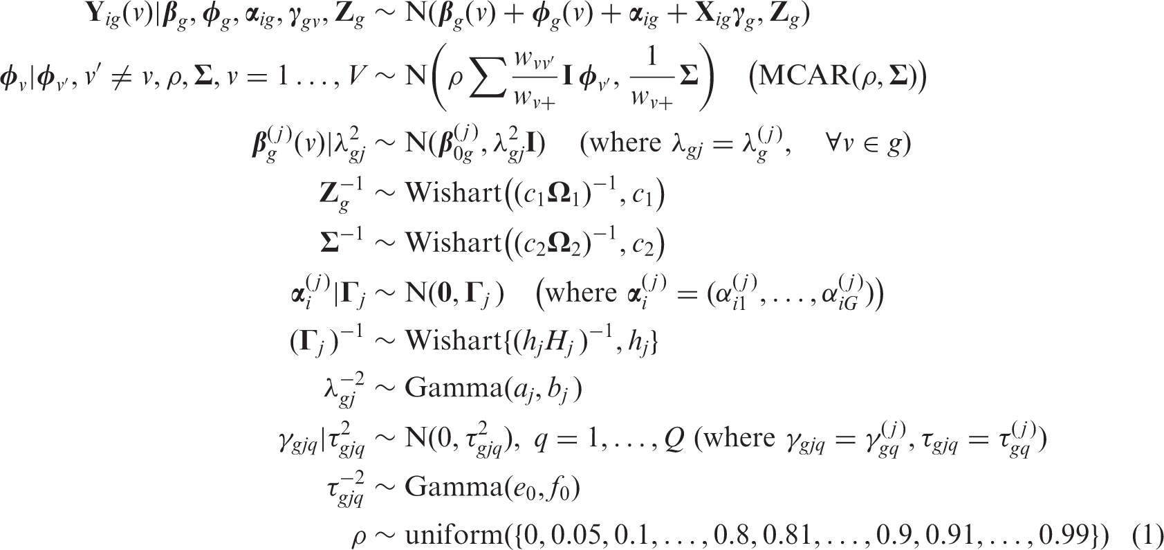Let $Y_{ig} (v) = (Y_{ig}^{(1)} (v), Y_{ig}^{(2)} (v))^{T}$ , where superscripts (1) and (2) denote the baseline and follow-up scans, respectively. Before processing, a local neighborhood of each voxel included in the analysis must be selected, for the voxel-level spatial modeling. We apply a three-dimensional (3D) neighborhood structure containing the 26 immediate neighboring voxels: 9 above, 9 below, and 8 adjacent. In addition, we consider only within-region neighbors. The neighborhood information is represented in a connectivity matrix W, where W = {w_vv′}_(V×V) is a symmetric matrix (i.e. w_vv′ = 1 if voxel v′ is in the defined 3D neighborhood of v), and w_v+ the sum of the elements in row v of W.

We propose a multivariate BHM that accounts for both spatial correlations between intra-regional voxels and between regions. The model also accounts for correlations between baseline and follow-up regional glucose use. In particular, our proposed model has the following hierarchical structure

Y_{ig} (v) | β_{g}, φ_{g}, α_{ig}, γ_{gv}, Z_{g} ~ N (β_{g} (v) + φ_{g} (v) + α_{ig} + X_{ig} γ_{g}, Z_{g}) φ_{v} | φ_{v'}, v' \neq v, ρ, Σ, v = 1 \dots, V ~ N (ρ \sum w_{vv'} w_{v +} I φ_{v'}, 1/ w_{v +} Σ) (MCAR (ρ, Σ)) β_{g}^{(j)} (v) | λ_{gj}^{2} ~ N (β_{0 g}^{(j)}, λ_{gj}^{2} I) (where λ_{gj} = λ_{g}^{(j)}, \forall v \in g) Z_{g}^{- 1} ~ Wishart ((c_{1} Ω_{1})^{- 1}, c_{1}) Σ^{- 1} ~ Wishart ((c_{2} Ω_{2})^{- 1}, c_{2}) α_{i}^{(j)} | Γ_{j} ~ N (0, Γ_{j}) (where α_{i}^{(j)} = (α_{i 1}^{(j)}, \dots, α_{iG}^{(j)})) (Γ_{j})^{- 1} ~ Wishart {(h_{j} H_{j})^{- 1}, h_{j}} λ_{gj}^{- 2} ~ Gamma (a_{j}, b_{j}) γ_{gjq} | τ_{gjq}^{2} ~ N (0, τ_{gjq}^{2}), q = 1, \dots, Q (where γ_{gjq} = γ_{gq}^{(j)}, τ_{gjq} = τ_{gq}^{(j)}) τ_{gjq}^{- 2} ~ Gamma (e_{0}, f_{0}) ρ ~ uniform ({0, 0.05, 0.1, \dots, 0.8, 0.81, \dots, 0.9, 0.91, \dots, 0.99})

(1)

where j denotes the scanning session (i.e. j = 1 denotes baseline and j = 2 follow-up session).

For each voxel v, the subject-specific quantities Y_ig(v) are assumed to vary randomly about a mean determined by a population-level mean parameter $β_{g} (v) = (β_{g}^{(1)} (v), β_{g}^{(2)} (v))^{T}$ , a population-level spatial dependence parameter φ_g(v) = $(φ_{g}^{(1)} (v), φ_{g}^{(2)} (v))^{T}$ , an individualized random effect component $α_{ig} = (α_{ig}^{(1)}, α_{ig}^{(2)})^{T}$ , and the covariates' parameters $γ_{g} = (γ_{g 1}^{(1)}, γ_{g 1}^{(2)}, \dots, γ_{gQ}^{(1)}, γ_{gQ}^{(2)})^{T}$ , where Q is the number of covariates in the model.

$X_{ig} = [X_{ig 1}^{(1)} 0 \dots X_{igQ}^{(1)} 00 X_{ig 1}^{(2)} \dots 0 X_{igQ}^{(2)}]$ is a 2 × 2Q matrix containing the mean-centered subject-specific covariates. We express vectors of random effects across the entire brain as $α_{i}^{(j)} = (α_{i 1}^{(j)}, \dots, α_{iG}^{(j)})$ , where j denotes the baseline and follow-up sessions, and $α_{i} = (α_{i 1}^{T}, \dots, α_{iG}^{T})^{T}$ . Given {β_g}, {φ_g}, {α_ig}, {γ_gv} and Z_g, the {Y_ig} are conditionally independent.

At the second level, the model expresses a prior belief that each voxel's population mean (for the jth session) arises from a normal distribution with a mean given by the overall region mean $β_{0 g}^{(j)}$ and variance $λ_{gj}^{2}$ . It represents a reasonable starting point to assume that voxels within anatomically defined regions exhibit brain activity that deviates around an overall mean for that region.

Spatial associations are introduced through random effects in the mean structure of the data. Bivariate spatial random effects at the voxel level call for an MCAR specification, where ρ is a scalar parameter representing the overall degree of spatial dependence and $1/ w_{v +} Σ$ the conditional covariance matrix between $φ_{v}^{(1)}$ and $φ_{v}^{(2)}$ . The connectivity (proximity) matrix W used in the MCAR prior for the spatial random effects φ is based on the 3D neighborhood structure described above.

The parameter ρ determines the magnitude of the spatial neighborhood effect. Following Gelfand and Vounatsou,8 we specify a discrete uniform prior for the spatial autoregression parameter ρ. We assume ρ < 1 to insure propriety; we do not allow ρ < 0 since this would violate the similarity of spatial neighbors which we seek, and we place prior mass which favors the upper range of ρ. In particular, we put equal mass on the following 36 values: 0, 0.05, 0.1,…, 0.8, 0.81, 0.82,…, 0.90, 0.91, 0.92,…, 0.99. In addition to the local MCAR correlations, we also have exchangeable within-region correlations introduced by the random effects structure.

The model also captures potential functional connections between anatomical brain regions through the covariance matrix Γ_j. We specify a conjugate inverse-Wishart prior for Γ_j, allowing a flexible unstructured covariance matrix. The multivariate structure enables us to compute the between-region connectivity matrix, separately for each session. Finally, hyperpriors on the MCAR parameters and other hyperparameters complete the model specification.

Estimation is performed using Markov chain Monte Carlo (MCMC) techniques implemented via Gibbs sampling. Applying MCMC methods in our context is complicated by the massive amount of data, the large number of spatial locations, and the large number of parameters that need to be estimated. The Gibbs-friendly model specification facilitates estimation by providing substantial reductions in computing time and memory. We present the full conditionals required to run the Gibbs sampler in the Appendix.

3.2 Prediction

We use the summary statistics (e.g. mean) from the posterior samples to predict the session 2 (6 months) scans for future patients, based on their baseline scans. The prediction proceeds as follows. We first draw the covariance matrix Γ from its full conditional distribution. We then draw α_i's, given Γ, from the prior distribution for α. Letting Y_i*_,1 denote the baseline scan and Y_i*_,2 the 6-month scan for a future subject, we have the necessary information (parameter estimates for β, φ, Γ, γ, Z, and α and the covariate matrix X) to estimate Y_i*_,2|Y_i*_,1.

At the region level, let $Y = (Y_{1}^{T}, Y_{2}^{T})^{T}$ , where Y₁ contains all the session 1 voxel values and Y₂ all the session 2 voxel values. For region g, then $Y_{g} = (Y_{g, 1}^{T}, Y_{g, 2}^{T})^{T} ~ N ((μ_{g, 1}^{T}, μ_{g, 2}^{T})^{T}, Σ_{g})$ , where $Σ_{g} = Z_{g} \otimes I_{V_{g}}$ .

From model (1), it follows that $Y_{i^{*}, 2} | Y_{i^{*}, 1} ~ N (b_{i^{*} g}, A_{i^{*} g})$ . For region g, $b_{i^{*} g} = μ_{i^{*} g, 2} +$ $Σ_{12}^{T} Σ_{11}^{- 1} (Y_{i^{*} g, 1} - μ_{i^{*} g, 1})$ and $μ_{i^{*} g} = β_{g} + φ_{g} + 1_{V_{g}} \otimes α_{i^{*} g} + 1_{V_{g}} \otimes X_{i^{*} gv} γ_{gv}$ . μ_i*g,2 is a vector consisting of even elements of μ_i*g. Writing $Z_{g} = [a c c b]$ , we see that $A_{i^{*} g} = b I_{V_{g}} - c I_{V_{g}} \cdot 1/ a I_{V_{g}} \cdot c I_{V_{g}} = (b - c^{2} a) I_{V_{g}}$ .

By inputting the posterior mean of the parameters obtained from the MCMC estimation, we obtain the estimated conditional mean ${\overset{\land}{b}}_{i^{*} g}$ and covariance matrix ${\overset{\land}{A}}_{i^{*} g}$ . The follow-up regional glucose uptake Y_g,2 is predicted using the mean of the estimated conditional distribution, i.e. ${\overset{\land}{b}}_{i^{*} g}$ . Also, a 100(1 − α)% prediction interval for Y_g,2 can be constructed based on the estimated conditional variance.

3.3 Model validation: Estimation of the prediction error

For each of the two groups (AD and HC) in the ADNI data, we applied our algorithm to predict the follow-up regional glucose uptake for 33 new (test) subjects using the estimated parameters from the training data. We quantify the prediction error by comparing the observed and predicted follow-up (6 months) brain activity. In neuroimaging, prediction of the brain activity is performed on each voxel, and the prediction error is evaluated across all voxels. Typical squared or absolute error functions are inappropriate since the brain activity measurement (such as regional glucose uptake or BOLD signal) has different baseline values across the brain. We propose the use of a scale-free loss function so that the prediction error is comparable across all brain voxels. The proposed function is the ratio of the square root of the prediction mean squared error (PMSE) and the average effects at voxel v. Specifically, this function (we will refer to it as the ‘standardized square root of the PMSE – stPMSE’) is defined as

stPMSE ({Y_{i}^{(2)} (v)}, {{\overset{\land}{Y_{i}}}^{(2)} (v)}) = \sqrt{(1 / N) \sum_{i = 1}^{N} [{\overset{\land}{Y_{i}}}^{(2)} (v) - Y_{i}^{(2)} (v)]^{2}} (1 / N) \sum_{i = 1}^{N} Y_{i}^{(2)} (v)

(2)

This measure of prediction error is similar to the measure proposed by Guo et al.1 We scale by an average of the observed, not the predicted values at voxel v; therefore, our measure will be more stable, e.g. against overestimated predicted values.

4 Results

We apply our Bayesian spatial hierarchical model to PET data from the study of AD (ADNI). We considered 39 regions relevant to AD in our analysis, which were selected from a set of 46 ROIs considered in Bowman et al.4 The complete list of regions with region sizes is given in Table A1, Supplementary Material (Available at: http://adni.loni.ucla.edu/wp-content/uploads/how_to_apply/ADNI_AcknowledgementList.pdf), Section 3. Areas of the temporal and limbic lobes are of particular interest since they were previously indicated as having either increased or decreased activity between at-risk subjects and controls in the first wave of the Alzheimer's data, or are thought to be involved with the verbal memory paradigm.10 We limit the number of regions in the analysis to be smaller than the number of subjects in the smallest group (in our case, 40) in order to reliably estimate the between-region covariance parameters.

Our model captures spatial correlations at three levels: (a) the short-range spatial correlation between voxels within a defined anatomic region, (b) exchangeable within-region correlations introduced by the random effects structure, and (c) the (potentially) long-range inter-regional connectivity, stemming from the covariance matrix Γ_j, of the random effect parameters α_ij. We specify a Wishart prior for $Γ_{j}^{- 1}$ .

For the inverse-Wishart prior, the degrees of freedom must satisfy h_j ≥ G to yield a proper prior distribution. This prior becomes more diffuse as h_j becomes smaller;11 hence, we set h_j = G to reflect the most diffuse proper prior that our data can support. A seemingly natural choice for H_j is a point estimate of Γ_j. We use the sample covariance matrix to obtain H_j, calculated from the subject-specific mean activity levels in each of the anatomical regions. In addition, we examine the sensitivity of our results to the sample covariance matrix by artificially reducing the correlations (covariances) using $H_{j}^{*} = (1 - w) H_{j} + w {diag (H_{j})} .$ We also use inverse-Wishart priors for Σ and Z_g, i.e. Σ⁻¹ ∼ Wishart((c₂Ω₂)⁻¹, c₂), $Z_{g}^{- 1} ~ Wishart ((c_{1} Ω_{1})^{- 1}, c_{1})$ , where Ω₁ and Ω₂ are 2 × 2 matrices and c₁ and c₂ shape parameters. Since we have no prior knowledge regarding the nature and extent of dependence, we choose Ω₁ and Ω₂ to be diagonal. In particular, we set Ω₁ = Ω₂ = I. The data will inform about dependence a posteriori. We set c₁ = c₂ = 4 to provide low precision for these priors.

To complete our BHM, we set a₁ = a₂ = 0.1, b₁ = 0.005, b₂ = 0.001, and h_j = G, resulting in vague or weakly informative priors, to insure that the information in the data primarily governs the results. However, more informative priors may be employed when fairly precise information is available.

To estimate the model parameters, we performed 3000 iterations with burn-in of 2000 iterations (5000 iterations in total) and thinning of five iterations (for storage and computation time). The programming was implemented in Matlab, and the computation was performed on a Linux cluster. The test/experiment environment consisted of an eight-core system with 16 GB of RAM. Each Matlab job was given a dedicated CPU and ran for approximately 26 h. Future optimizations include taking advantage of the multithreaded nature of several Matlab image analysis functions or using the Matlab Distributed Computing Environment to use multiple cores per job for speed improvements.

Due to a large number of parameters in our model, it is impractical to monitor the trace plots for each of the parameters. Also, running parallel chains is recommended to monitor how the chains mix. We obtained trace plots for a number of randomly selected voxels in several regions, for each of the voxel-level parameters. Several plots and histograms are given in Supplementary Material, Section 3. The chains obtained from the Gibbs sampler (trace plots) are satisfactory, i.e. the generated Markov chains seem to converge, after the burn-in period, to our distributions of interest. We also monitored the trace plots for other (region-specific and scalar) parameters and found them to be satisfactory.

4.1 Prediction of brain activity for PET data from a study of AD (ADNI)

We apply the proposed prediction algorithm to forecast the follow-up regional glucose uptake for each of the subjects in the test dataset, which consists of 33 subjects in each group. Our algorithm provides individualized predictions of the regional glucose uptake, based on the unique information in each subject's baseline scan and relevant personal characteristics (e.g. ADAS-cog score). For prediction, we estimate the covariate effect at the second scanning session by the mean of the second session in the training data. For both groups (AD and HC), the posterior mean of the spatial effect ρ was 0.99, for both scanning sessions, indicating very strong spatial dependence. Also, estimated covariance matrices between the baseline and follow-up regional glucose uptake at a region level, Z_g, yield high between-session correlations (> 0.7 for almost all regions) at a region level.

4.1.1 Individualized prediction maps

Figure 1 shows the individual prediction maps of the regional glucose uptake at 6 month follow-up for four selected AD patients. The prediction maps for several other subjects are given in Supplementary Material, Section 3. We see that there are notable differences between subjects in the predicted follow-up activity, indicating that possibly different stages of the disease are present in those individuals. We compare the individual predicted maps (Figure 1(a)) to the observed maps (Figure 1(b)) and notice a strong agreement between the observed and predicted brain activity. Similar correspondence is observed for most of the subjects. The individual prediction maps, such as those in Figure 1(a), highlight possible individual differences in the progression of the disease.

Figure 1.

Individualized predicted (a) and observed (b) 6-month follow-up regional glucose uptake measurements for four AD patients from the test dataset. Axial slice 40 is shown in radiological view. There is a satisfactory agreement between the observed and predicted 6-month regional glucose uptake.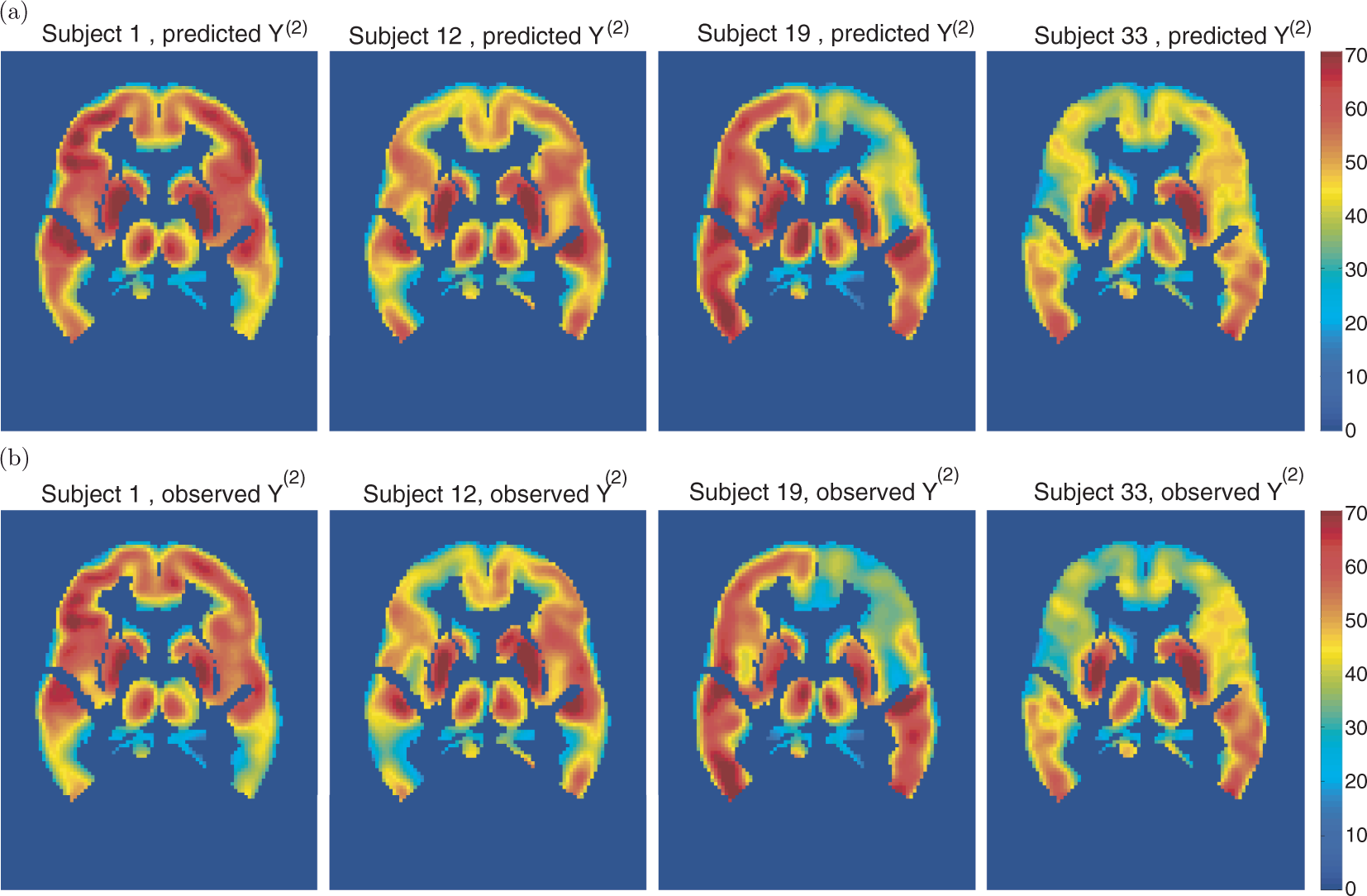

We also predict the follow-up brain activity for the HC test dataset, which consisted of 33 subjects. The results for four selected subjects are given in Figure 2. Similar satisfactory agreement is observed between the predicted and observed maps. We also notice that this group exhibits smaller between-subject differences than the AD group.

Figure 2.

Individualized predicted (a) and observed (b) 6-month follow-up regional glucose uptake measurements for four HC subjects from the test dataset. Axial slice 40 is shown in radiological view. There is a satisfactory agreement between the observed and predicted 6-month regional glucose uptake.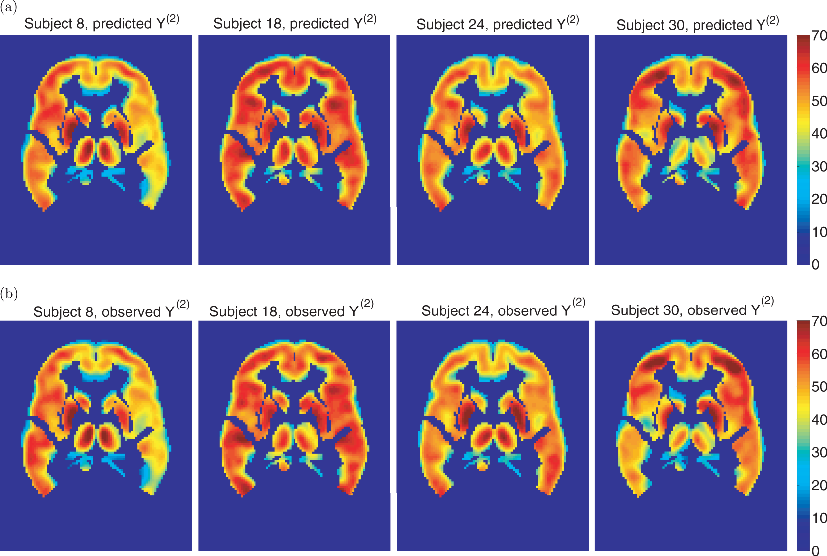

4.2 Comparisons with competing prediction models

We compare our prediction results with the results obtained using three proposed competing methods: the general linear model (GLM)12 based method, the method based on the BHM proposed in Guo et al.,1 and the method based on the Bayesian spatial hierarchical model for activation and connectivity (BSMac) analysis proposed in Bowman et al.4 and Zhang et al.5

Comparison with predictions based on the GLM. The GLM models the brain activity for all subjects using common population parameters. Independence and sphericity between scans at baseline and follow-up are assumed. Estimates from the GLM are obtained using ordinary least squares. The predicted follow-up brain activity reflects only the population-level expectation and does not take into account the information from the subject's pretreatment scans. That is, $Y_{g, 2}^{*} = X_{g, 2}^{*} \cdot \overset{\land}{β_{g}}$ , where subscript 2 denotes session 2 (follow-up) brain activity at region g, superscript * the new subject, and $\overset{\land}{β_{g}}$ the estimate of the session 2 mean parameter obtained from the training dataset. Figure 3(d) displays the square root of the PMSE, relative to the average brain activity, based on the GLM.

Figure 3.

The images depict the square root of the PMSE, divided by the average observed brain activity (stPMSE, (2)) at each voxel for prediction of the follow-up activity for 33 test subjects in the AD group. Axial slices 35, 40, and 45 are shown (in radiological view) of the stPMSE map based on (a) our proposed model; (b) BHM proposed in Guo et al.1; (c) BSMac proposed in Bowman et al.4; and (d) GLM. Average errors: 0.083 for the BSPM (a), 0.080 for the BHM (b), 0.104 for the BSMac (c), and 0.156 for the GLM (d). stPMSE: standardized square root of the prediction mean squared error; AD: Alzheimer's disease; BSPM: Bayesian spatial prediction model; BHM: Bayesian hierarchical model; BSMac: Bayesian spatial hierarchial model for activation and connectivity; and GLM: general linear model.

Comparison with prediction based on BSMac. The prediction algorithm based on the BSMac is defined in a way similar to the algorithm based on our proposed Bayesian spatial prediction model (BSPM). Since BSMac does not estimate the correlations between baseline and follow-up brain activity scans (Y_i's ), i.e. temporal correlations, we estimate these using the sample covariances, at the voxel level. The local spatial parameters are also not estimated and are dropped from the estimated conditional mean. Figure 3(c) displays the square root of the PMSE, relative to the average brain activity, based on the BSMac.

Comparison with predictions based on the BHM. The prediction based on the BHM proposed in Guo et al.1 enables individualized follow-up predictions of brain response by incorporating the unique information in each subject's baseline functional brain scans and other relevant personal characteristics (covariates). The model also captures the correlations between baseline and follow-up brain activity scans, which enables a similar prediction algorithm to ours. Figure 3(b) displays the square root of the PMSE, relative to the average brain activity, based on the BHM.

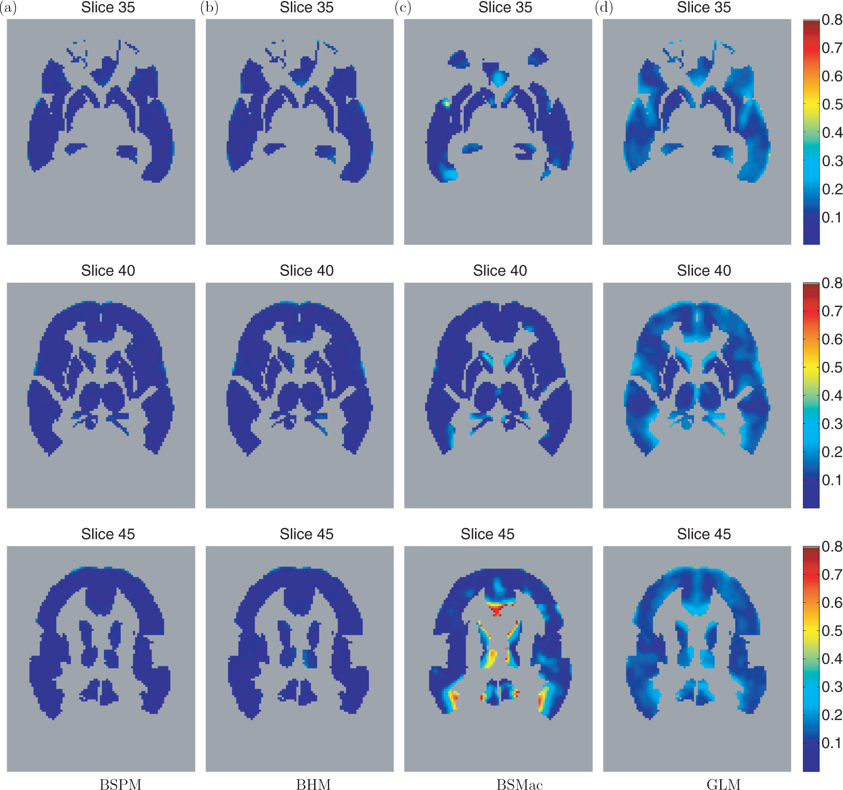
A comparison between Figure 3(a) and (d) indicates that prediction errors based on our proposed model are lower than those from the GLM, on average. The average error (total sum over all voxels, divided by the number of voxels included in the analysis), for the model based on the GLM is 0.156. Also, the superiority of our prediction model is consistently observed across the brain. A comparison between Figure 3(a) and (c) indicates that the prediction errors based on our proposed model are also lower than those from the BSMac, on average. We also notice improvement over the GLM model. The average errors are 0.083 for the BSPM, 0.080 for BHM, 0.104 for the BSMac, and 0.156 for the GLM-based prediction method.

While, for some subjects in this study, there is a strong similarity between the baseline and the 6-month scans, our model draws more predictive power than the prediction based on the baseline scans only. The average error (the whole-brain accuracy) for the ‘baseline only prediction’ (calculated using equation (2)) is 0.085, compared to 0.083 for our method. Likely, larger differences would occur for the 24-month follow-up images, when compared to baseline. We give more details and show figures with the baseline, the observed, and the predicted follow-up (6 months) images, for some selected subjects, in the Supplementary Material, Section 3.

A comparison between Figure 3(a) and (b) indicates that, for these experimental data, the prediction errors based on our proposed model and the model proposed in Guo et al.1 are very comparable (the difference in average errors is in the third decimal place). However, an additional advantage of our approach is that inter-regional functional correlations can be estimated through the covariance matrix Γ_j. The functional connectivity maps in Figure 4 display selected brain regions, with lines connecting regions that have (posterior median) correlations exceeding 0.75. The line thicknesses depend on the strengths of the inter-regional correlations.

Figure 4.

Region functional connectivity for AD (top) and HC (bottom) subjects. The regions that have (posterior median) correlations exceeding 0.75 are shown. The connecting lines have different thickness, corresponding to the strength of the inter-regional correlations. AD: Alzheimer's disease; HC: healthy controls.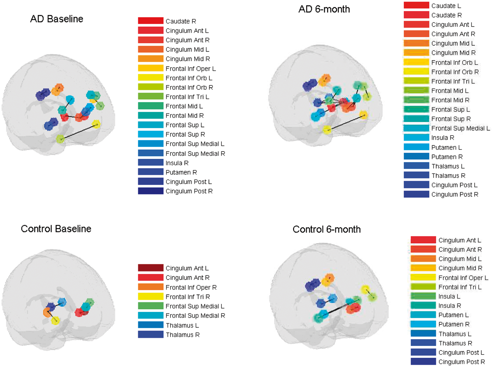

5 Simulation

We performed a small simulation study to evaluate the accuracy of our estimation procedure. To generate data for the simulations, we selected five regions from the automated anatomical labeling map7 (regions 79, 73, 15, 13, and 85) with sizes ranging from 234 to 4655 voxels and simulated data for 15 subjects. We used our experimental data described in Section 2 to specify the true values for β_g, spatial parameters φ_g, random effects parameters α_i, and the covariate parameters γ_g. The rest of the (hyper)parameters were drawn from the prior distributions specified in the model. After all the parameters that define the mean and the covariance parameters in model (1) were specified, 200 simulated datasets were drawn, with the specified mean parameters and the variance–covariance matrix. We then applied our estimation procedure to each of the datasets and analyzed the posterior distributions of the parameters. Table 1 summarizes the results for the parameters of the covariance matrix Z_g, for each of the five selected regions. We see that the biases for the covariance matrix parameters Z_g are small, for each of the regions. In addition, the spatial parameter ρ has only a small bias: we set the true value in the simulated datasets to 0.9 and the mean of the estimated ρ, across 200 datasets, was found to be 0.9134 (for each dataset: we first find a median of the parameter's posterior distribution, then average those medians). Posterior means of the estimated voxel-level parameters (for randomly selected 25 voxels in each region) as well as the posterior means of the random effects α_ij are presented in the Supplementary Material, Section 4.

Table 1.

Summary of the simulation results for the parameters in the covariance matrix Z_g, for each region.

Region
1		2		3		4		5
Parameter	True	Estimated	True	Estimated	True	Estimated	True	Estimated	True	Estimated
$Z_{g}^{11}$	323.26	321.25	160.61	160.05	11.46	11.46	3.44	3.44	3.57	3.57
$Z_{g}^{22}$	120.75	120.50	45.30	45.15	37.22	37.19	10.45	10.45	3.38	3.38
$Z_{g}^{12}$	−41.95	−41.40	−33.70	−33.43	16.32	16.30	4.08	4.08	2.40	2.40

$Z_{g}^{11}$ and $Z_{g}^{22}$ denote the variance, and $Z_{g}^{12}$ the covariance components.

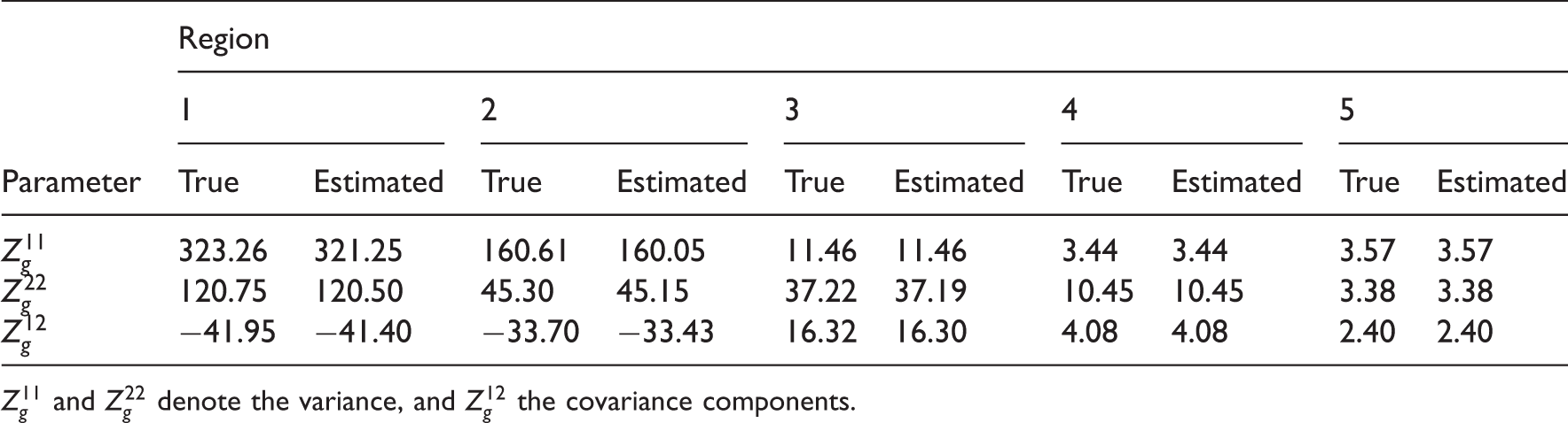
Parameters that are most relevant to the prediction (β's, φ's, α's, Z_g) have small or relatively small biases, while the parameters that contribute to the prediction less directly, have larger biases.

6 Discussion

In this article, we describe a framework for spatiotemporal modeling of functional neuroimaging data that provides important advantages over some previously proposed methods. We develop a novel method for predicting post-baseline (or follow-up) brain scans, based on the baseline scans. The prediction algorithm is based on a novel hierarchical Bayesian spatial model formulation. Our method is applicable in many clinical situations (e.g. for predicting the progression of a disease, or to predict after-treatment brain activity, based on baseline pre-treatment activity). The proposed method may be useful in clinical situations where it is too costly to acquire multiple (repeated) scans on subjects.

Our model builds on the predictive model proposed by Guo et al.,1 and a spatial BHM proposed by Bowman et al.,4 by incorporating a proper MCAR prior for the spatial effect. The proposed model captures the short-range correlations between voxels within a defined anatomical region as well as the (potentially) long-range inter-regional correlations, which provide information about functional connectivity between brain regions. We consider a 3D neighborhood structure for estimation of the local spatial associations.

Based on the proposed model, we formulate a prediction algorithm for the follow-up brain activity, based on an individual's baseline functional neuroimaging data and relevant subject-specific characteristics. By borrowing strength from the spatial information, our approach achieved improved predictive performance when compared with the GLM and BSMac approaches. Our prediction method is comparable to the method developed in Guo et al.,1 but it offers some additional advantages, e.g. estimation of long-range inter-regional spatial correlations through the covariance matrix Γ_j (Figure 4).

We apply our Bayesian spatial hierarchical model to PET data from a study of AD, but the same methodology can easily be applied to data obtained from an fMRI study. In that case, individual summary statistics (i.e. regression coefficients) from a typical first stage GLM-based fMRI data analysis would first be obtained (in practice often obtained using software packages such as SPM or FSL), and then used as Y's in our model (1).

One of the limitations of our proposed method is that the computing time is very long (even for a relatively small number of iterations such as 5000) for the estimation part of the algorithm. However, this step is done once, and the prediction step is very fast (on the order of seconds per individual). Computing time can be improved by implementing some parallel computing steps (as described in Section 4). Another limitation is that we employ a separable bivariate spatial model, for computational reasons and simplicity. Using two separate spatial effect parameters could be considered in future work to determine if spatial dependence differs across scanning sessions.

We note that the estimation was sensitive to the selection of initial values for certain priors, in particular to various specifications of the inverse gamma and inverse Wishart prior parameters and some care is needed when selecting values to avoid numerical problems in the estimation procedure. We tried several different combinations of initial values for e.g. a₁, a₂, b₁, b₂ that result in weakly informative priors which did not cause any estimation problems, and the posterior estimates were consistent across these prior specifications. Correlations calculated from Γ_j were more variable, but still relatively consistent. A more thorough sensitivity analysis to examine the robustness of our findings to various specifications of the prior parameters would require a substantial computational time, and this will be considered in future work.

Some recent studies13^–15 have found that the β-amyloid protein 1-42, total tau protein, and phosphorylated tau_181P protein concentrations, each derived from cerebral spinal fluid in the brain, may be clinically relevant biological markers for the differential diagnosis of AD. These biological measures may, therefore, serve as potentially useful covariates (predictors) in our model. Some of these proteins were collected in the ADNI study, but the rate of missing data (among subjects with FDG-PET scans) was too substantial for inclusion in our analysis.

Footnotes

Acknowledgments

The authors are grateful to Dr Ying Guo from the Department of Biostatistics and Bioinformatics at Emory University for valuable discussions and constructive comments.

Data collection and sharing for this project was funded by the Alzheimer's Disease Neuroimaging Initiative (ADNI) (National Institutes of Health grant U01 AG024904). ADNI is funded by the National Institute on Aging, the National Institute of Biomedical Imaging and Bioengineering, and through generous contributions from the following: Abbott; Alzheimer's Association; Alzheimer's Drug Discovery Foundation; Amorfix Life Sciences Ltd; AstraZeneca; Bayer HealthCare; BioClinica, Inc.; Biogen Idec Inc.; Bristol-Myers Squibb Company; Eisai Inc.; Elan Pharmaceuticals Inc.; Eli Lilly and Company; F. Hoffmann-La Roche Ltd and its affiliated company Genentech, Inc.; GE Healthcare; Innogenetics, N.V.; IXICO Ltd.; Janssen Alzheimer Immunotherapy Research & Development, LLC.; Johnson & Johnson Pharmaceutical Research & Development LLC.; Medpace, Inc.; Merck & Co., Inc.; Meso Scale Diagnostics, LLC.; Novartis Pharmaceuticals Corporation; Pfizer Inc.; Servier; Synarc Inc.; and Takeda Pharmaceutical Company. The Canadian Institutes of Health Research is providing funds to support ADNI clinical sites in Canada. Private sector contributions are facilitated by the Foundation for the National Institutes of Health (). The grantee organization is the Northern California Institute for Research and Education, and the study is coordinated by the Alzheimer's Disease Cooperative Study at the University of California, San Diego. ADNI data are disseminated by the Laboratory for Neuro Imaging at the University of California, Los Angeles. This study was also supported by NIH grants P30 AG010129 and K01 AG030514.

Funding

This study was supported by NIH grants R01-MH079251 (Bowman) and NIH predoctoral training grant T32 GM074909-01 (Derado).

References

Guo

Bowman

Kilts

. Predicting the brain response to treatment using a Bayesian hierarchical model with application to a study of schizophrenia. Hum Brain Mapp 2008; 29: 1092–1109.

Stonnington

Chu

Klöppel

. Predicting clinical scores from magnetic resonance scans in Alzheimer's disease. NeuroImage 2010; 51(4): 1405–1413.

Marquand

Howard

Brammer

. Quantitative prediction of subjective pain intensity from whole-brain fMRI data using Gaussian processes. NeuroImage 2010; 49(3): 2178–2189.

Bowman

Caffo

Bassett

. A Bayesian hierarchical framework for spatial modeling of fMRI data. NeuroImage 2008; 39: 146–156.

Zhang

Agravat

Derado

. BSMac: a MATLAB toolbox implementing a bayesian spatial model for brain activation and connectivity. J Neurosci Methods 2012; 204: 133–143.

Mueller

Weiner

Thal

. The Alzheimer's disease neuroimaging initiative. Neuroimaging Clin N Am 2005, pp. 15–15.

Tzourio-Mazoyer

Landeau

Papathanassiou

. Automated anatomical labelling of activations in SPM using a macroscopic anatomical parcellation of the MNI MRI single subject brain. NeuroImage 2002; 15: 273–289.

Gelfand

Vounatsou

. Proper multivariate conditional autoregressive models for spatial data analysis. Biostatistics 2003; 4(1): 11–25.

Brodmann K. Vergleichende Lokalisationlehre der Grosshirnrinde in ihren Prinzipien Dargestellt auf Grund des Zellenbaues, translated by Garey LJ as Brodmann's Localisation in the cerebral cortex. London: Smith-Gordon, 1994 [original publication date 1909].

10.

Bassett

Yousem

Christinzio

. Familiar risk for Alzheimer's disease alters fMRI activation patterns. Brain 2006; 129: 1229–1239.

11.

West

Harrison

. Applied Bayesian forecasting and time series analysis, Boca Raton, FL: Chapman and Hall/CRC, 1989.

12.

Friston

Holmes

Worsley

. Statistical parametric maps in functional imaging: A general linear approach. Hum Brain Mapp 1995; 2(4): 189–210.

13.

De Meyer

Shapiro

Vanderstichele

. Diagnosis-independent Alzheimer disease biomarker signature in cognitively normal elderly people. Arch Neurol 2010; 67(8): 949–956.

14.

Anoop

Singh

Jacob

. CSF biomarkers for Alzheimer's disease diagnosis. Int J Alzheimer's Dis 2010; 2010: 606802–606802. . DOI: 10.4061/2010/606802.

15.

Buerger

Zinkowski

Teipel

. Differential diagnosis of Alzheimer disease with cerebrospinal fluid levels of tau protein phosphorylated at threonine 231. Arch Neurol 2002; 59(8): 1267–1272.

Supplementary Material

Please find the following supplemental material available below.

For Open Access articles published under a Creative Commons License, all supplemental material carries the same license as the article it is associated with.

For non-Open Access articles published, all supplemental material carries a non-exclusive license, and permission requests for re-use of supplemental material or any part of supplemental material shall be sent directly to the copyright owner as specified in the copyright notice associated with the article.

0.00 MB

0.25 MB