Modeling height for children born small for gestational age treated with growth hormone

Abstract

The analysis of growth curves of children can be done on either the original scale or in standard deviation scores. The first approach is found in many statistical textbooks, while the second approach is common in endocrinology, for instance in the evaluation of the effect of growth hormone in children that are born small for gestational age that remain small later in childhood. We illustrate here that the second approach may involve more complex modeling and hence a worse model fit.

Keywords

Longitudinal studies human growth height Bayesian models growth hormones standard deviation scores

1 Introduction

Children that are born small for gestational age (SGA) and do not show catch-up growth are eligible for treatment with a growth hormone (GH). Although there is some concern that this growth hormone might adversely affect the metabolism, generally the treatment is considered to be safe and effective.^1–3 However, since the cost of treatment with growth hormone is relatively high,⁴ it is of practical interest to know the dose that achieves optimum growth. For children under treatment it is important to predict their adult height in order to avoid unrealistic expectations.

In this article, we focus on SGA children treated with growth hormone and consider (1) modeling of height as a function of age and (2) the prediction of the adult height. We note that in the endocrinology literature modeling the height is usually done in terms of the standard deviation score (SDS).^5–15 There is only a minority of studies that model the untransformed height.¹⁶ A few studies are based on a combination of both scales.^17,18 In order to model the growth curve of height y in SDS, for each age the mean and standard deviation of y need to be established in the reference population. That is, at age t one determines μ(t, s) and σ(t, s), which are the mean and standard deviation of y respectively, in the reference population at age t and for sex s. A variety of techniques can be employed to determine μ(t, s) and σ(t, s) of which the most prominent seems to be Cole's LMS method.^19,20 For most of these techniques some kind of smoothing is involved. For a new child with height y₀ determined at age t₀, the height can be expressed in SDS by computing $y_{0} - μ (t_{0}, s_{0}) σ (t_{0}, s_{0})$ with s₀ the gender of that child. Note that the reference population most often consists of children with no diagnosed growth retardation problems.^21,22 When the distribution of y_t,s is not normal, computation of the SDS is slightly more complicated, involving a transformation of the raw scores. Here we will assume that height has a normal distribution conditional on the covariates (as a conditional normal distribution is often used in practice to model height and seems to work quite well.)

Presenting the height in SDS allows to conclude readily how remote the child's height is from its expected height. Further, for a child belonging to the reference population, the expected growth curve in SDS is more or less a horizontal line before it reaches puberty, a phenomenon called ‘tracking’.²³ Expressing height on the SDS scale aims to produce profiles that are easy to model. However, for children with an abnormal growth pattern, such as SGA children, the SDS profile is typically (highly) nonlinear. Thus, a modeling exercise examining factors that influence growth in SGA children will typically be more complex on the SDS scale than on the height scale. This might adversely affect the power of the study. Here we illustrate, using data of a double blinded randomized trial in SGA children conducted in the Netherlands, that it could be preferable to model the height on the original scale.

To model the growth curves, we used a Bayesian approach with WinBUGS (version 1.4.3). The advantage of Markov Chain Monte Carlo (MCMC) techniques over classical nonlinear mixed effects maximum likelihood estimation are (1) less dependence of the modeling exercise on the starting values of the parameters; (2) more flexibility with respect to distributional assumptions for the random effects. Further, the Bayesian approach has two additional advantages: (3) taking into account all uncertainty involving the estimation of model parameters when predicting characteristics of individual growth curves and (4) the ability to include prior information into the sampling algorithm. Moreover, (5) Bayesian statistical inference does not need to be based on large sample arguments but is simply derived from the posterior distribution of the parameters.

The article is organized is follows: section 2 describes the study and the growth data. In section 3 we introduce the class of models considered in this exercise. In section 4 we apply the models to the data and evaluate the models with regard to their prediction characteristics. We conclude the article with a discussion.

2 The Dutch growth hormone trial data

The Dutch growth hormone (DGH) trial^24,25 was the first randomized double blind trial in the Netherlands that investigated the effect of the dose of growth hormone treatment on the growth of children that were born SGA without spontaneous catch-up growth (so they were still too small at the start of the trial). In this study, SGA is defined as having a birth length below the third percentile of the normal Dutch population at birth. A number of factors can cause a child to be SGA such as: intrauterine exposure to toxins, infections, chromosomal disorders, congenital defects, metabolic diseases and genetic disorders, the use of tobacco or alcohol by the mother, certain diseases of the mother or certain factors jeopardizing placental perfusion. Often, however, the exact underlying cause remains unclear.²⁶ SGA children may show catch-up growth, i.e. while they are initially small, often they grow faster than other children of the same gestational age such that within their first year of age their height lies within the 95% normal range. However, some SGA children experience no catch-up growth and remain too small for their age.²⁷ These children may experience several medical problems later in life such as: an increased risk of developing hypertension, dyslipidemia, impaired glucose tolerance or diabetes mellitus.²⁸

The DGH trial started in 1991. One group of children was treated with 1 mg GH/(m² day) (low dose) and the other with 2 mg /(m² day) (high dose) of a synthetic growth hormone (Norditropin®). Inclusion criteria were: boys between 3 and 11 years of age or girls between 3 and 9 years of age with a birth length below −1.88 SDS, a height below −1.88 SDS at the start of the trial (the SDS scores are computed using the reference values by Roede and van Wieringen²⁹), no spontaneous catch-up growth in the last year, pre-pubertal stage and an uncomplicated neonatal period without severe asphyxia, sepsis or lung problems. Children with endocrine or metabolic disorders, chromosomal disorders or growth failure caused by other disorders and syndromes as well as children that used drugs that could interfere with growth hormones were excluded. Treatment should be stopped as soon as the child reaches adult height. For this purpose adult height was defined as the height of a child at the measurement at which the growth over the previous 6 months was less than half a centimeter.

In total 79 children were included in the trial, 52 boys and 27 girls. The average age at the start of treatment was 7 years and 3 months. Nine children dropped out of the study before reaching adult height: 4 because of lack of motivation, 3 children stopped after they moved, 1 stopped because of signs of precocious puberty and 1 because of signs of growth hormone insensitivity. For 51 of the 70 children who started growth hormone treatment, an extra height measurement was taken about 5 years after the treatment was discontinued. This measurement can sometimes be a little higher than the last regular measurement. No further measurements where taken after this extra measurement, because the investigators were convinced that adult height was reached.

The DGH data have been analyzed before. Sas et al.²⁴ looked at the height of the children in the 5 years after the start of this study by comparing the average height SDSs between the treatment groups and with the previous year in all of the first 5 years of follow up by means of t-tests. The height SDSs were also compared with −1.88 (the 3rd percentile) to see whether the children were within the normal range. The authors concluded that almost all children were within the normal range after 5 years of GH treatment. Further, there was no significant difference between the average height SDS of the two dose groups at the end of the 5-year treatment period.

van Pareren et al.²⁵ looked at the 54 children that had reached adult height at the time of their exploration. The average adult height SDS in each treatment arm was compared with the average height SDS before study, and with zero (to see whether the mean adult heights are the same as in the reference population). The mean adult height SDSs were also compared between treatment arms. All comparisons were done using t-tests. In both groups there was an increase in average height SDS but not significantly different between the treatment arms. In the high dose group the average adult height SDS did not differ from zero.

The aims of Sas et al.²⁴ and van Pareren et al.²⁵ differ from the aims in this study since we want to make use of the whole growth curve to compare treatment doses. In other words we wish to build a growth curve model for the heights.

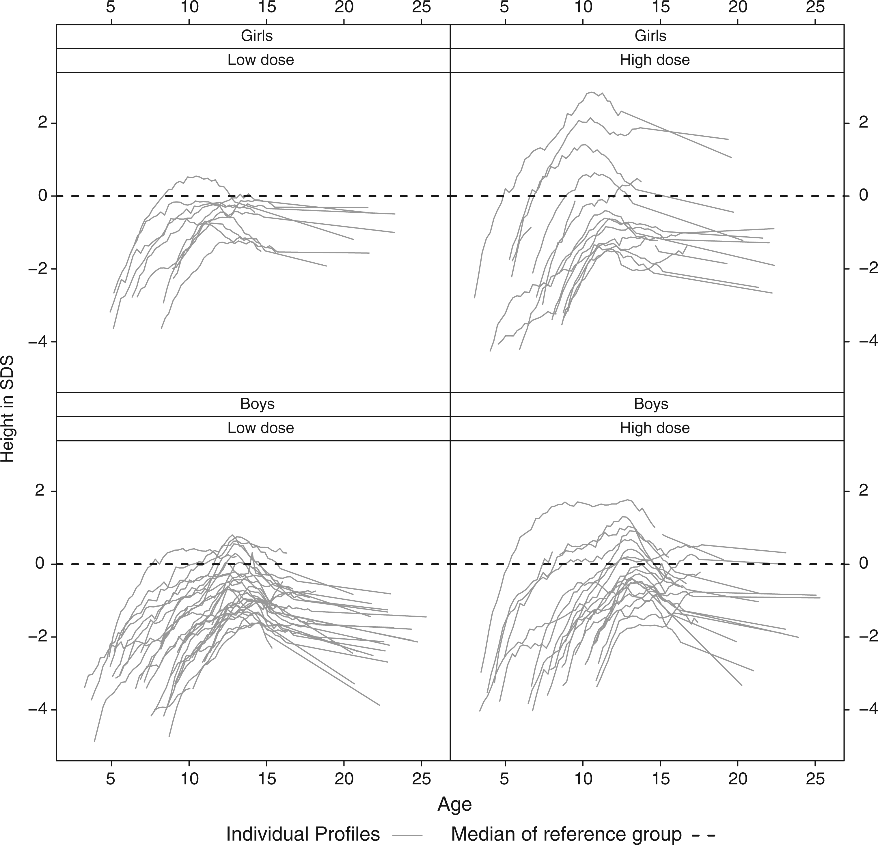
In Figure 1 the height profiles of the children participating in the DGH trial are displayed. The average height in the reference population has been added as a benchmark. When expressed in SDS the profiles look as in Figure 2.

Figure 1.

Dutch growth hormone trial: height profiles in cm split up according to gender and dose administration.

Figure 2.

Dutch growth hormone trial: height profiles in standard deviation score split up according to gender and dose administration.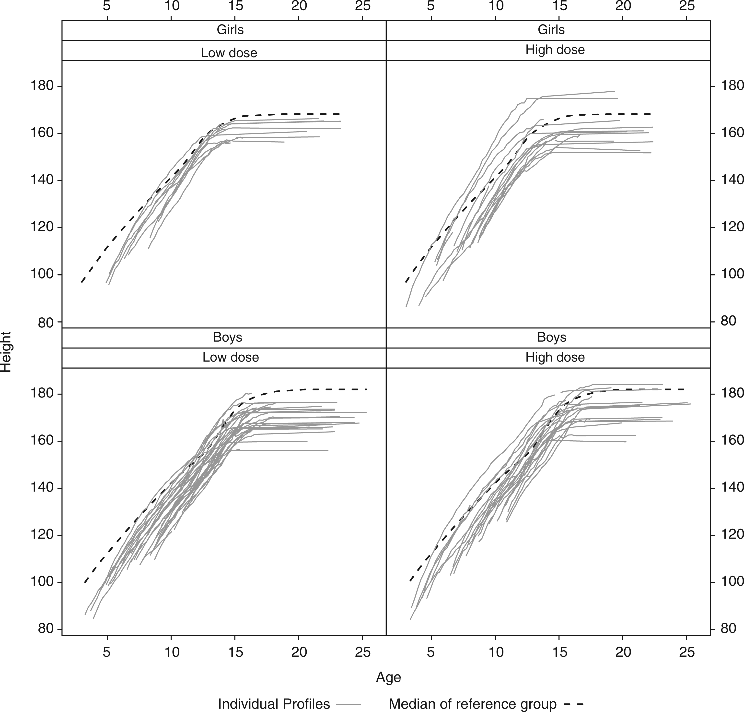

3 Statistical models for the height profiles

We consider two growth curve approaches to model height as a function of age: (1) the untransformed height (in centimeters) and (2) in SDS. All modeling was done by calling WinBUGS from R using the R2WinBUGS package.

3.1 Modeling the height in centimeters

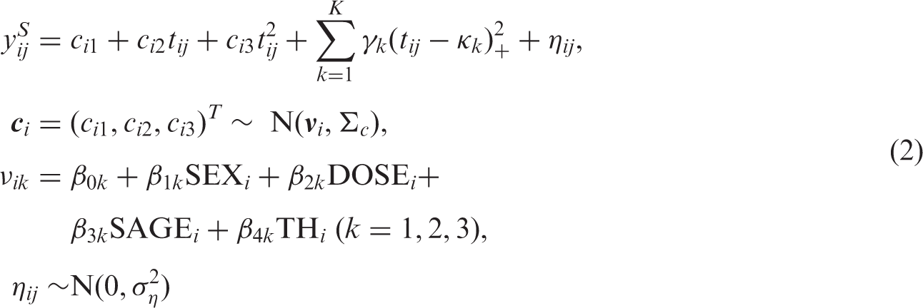
Figure 1 suggests a suitable structure for a model of height as a function of age. The height of each child follows an almost linear pattern until the adult height is reached. On closer inspection, the linearity of the initial part of the growth curve can be improved upon by a square root transformation of age (as confirmed by DIC). Hereby the individual growth curves appear approximately as broken lines. For this reason, we assumed that the child's height can be described by an initial phase of linear growth (in terms of the square root of age) until maturity is reached at which growth stops and a horizontal line appears. Hence we assumed that an individual's growth curve can be described by an intercept, the slope of the initial phase and the age at which growth stops. Further, we assumed that these three subject-specific coefficients have a trivariate normal distribution with a mean possibly depending on sex, treatment dose, age at start of the treatment and the target height SDS (TH) of the child. The target height is the midparental height, i.e. the average height of the parents, corrected for the sex of the child and corrected for the secular growth trend (meaning that on average each generation is taller than the previous one). To this model measurement error is added. Our model for height now looks as follows

\begin{matrix} y_{i j} = b_{i 1} + b_{i 2} \min (t_{i j} - b_{i 3}, 0) + ε_{i j}, \\ b_{i} = (b_{i 1}, b_{i 2}, b_{i 3}) T \sim N(μ_{i}, Σ_{b}), \\ μ_{i k} = α_{0 k} + α_{1 k} {SEX}_{i} + α_{2 k} {DOSE}_{i} + α_{3 k} {SAGE}_{i} + α_{2 k} {TH}_{i} (k = 1, 2, 3), \\ ε_{i j} \sim N (0, σ_{ε}^{2}) \end{matrix}

(1)

In (1) y_ij is the height of the ith child at age_ij, (j = 1,…, n_i; i = 1,…, n), the age is transformed

t_{i j} = \sqrt{{age}_{i j}} - \sqrt{20}

. Where 20 is the age where all children reach adult height. b_i1, b_i2 and b_i3 are the subject-specific parameters of the growth curve of the ith child, and indicate respectively the adult height, slope and change point for the ith child. The vector b _i is assumed to have a trivariate normal distribution with mean μ_i and covariance matrix Σ_b. We assume that μ_ik, the kth component of μ_i, is a linear function of covariates with weights α_hk, with h = 0,…, 4. The measurement error ϵ_ij is assumed to follow a normal distribution with zero mean and variance

σ_{ε}^{2}

. Dose is coded as −1 for the low dose and 1 for a high dose, sex is coded −1 for boys and 1 for girls. SAGE_i is the age of entry age_i0, approximately centered by subtracting 7 from it. By centering the covariates, we obtained better convergence properties for the MCMC chains.³⁰

Vague and conjugate priors were taken for all fixed effect parameters i.e. independent normal priors with zero mean and large (10⁶) variance for the αs, an inverse Wishart prior with 3 degrees of freedom and an identity scale matrix for the covariance matrix of the random effect parameters b and an inverse gamma prior with rate 0.001 and mean 0.001 for the residual variance $σ_{ε}^{2}$ .

3.2 Modeling height on the SDS scale

The growth curves in SDS show a more complex behavior than those on the original scale. From the profiles in Figure 2 we observe that initially the SGA children under growth hormone treatment grow much faster than normal children of the same age, so their SDS increase. But afterwards the growth rate (in SDS) slows down. Eventually, the height SDS even decreases, because the children stop growing at an age where some children in the reference population still continue to grow.

Because we do not see an obvious structure in the SDS profiles, the mean of the SDS curves is modeled with a quadratic spline³¹ augmented with subject specific random intercepts, random slopes and a random quadratic part. In this way the number of random terms is the same as for the change point model 1. Furthermore, the SDS–growth curves have a quadratic appearance so a quadratic function seems a logical choice when we want to model the growth curves with splines with a low number of knots. We have defined t_ij as the square root of age_ij after standardization. The number of knots can be increased to make the model more flexible. We included the same covariates as those for modeling the height in centimeters. So we have the following model

\begin{array}{l} y_{i j}^{S} = c_{i 1} + c_{i 2} t_{i j} + c_{i 3} t_{i j}^{2} + \sum_{k = 1}^{K} γ k {(t_{i l} - k_{k})}_{+}^{2} + η_{i j}, \\ c_{i} = {(c_{i 1}, c_{i 2}, c_{i 3})}^{T} \sim N (ν_{i}, \sum_{c}), \\ ν_{i k} = β_{0 k} + β_{1 k} {SEX}_{i} + β_{2 k} {DOSE}_{i} + β_{3 k} {SAGE}_{i} + β_{4 k} {TH}_{i} (k = 1, 2, 3), \\ η_{i j} \sim N (0, σ_{η}^{2}) \end{array}

(2)

y_{ij}^{S}

is the height of the ith child at age_ij expressed as SDS with the general Dutch population stratified by sex as in Roede and van Wieringen.²⁹ The coefficients c_i1, c_i2 and c_i3 denote respectively the intercept, slope and quadratic term for the ith child that are added to the general pattern. The γs are coefficients of the spline function that do not vary across individuals. The notation,

(x) 2 +

indicates x² when x > 0 and 0 otherwise. The κ_ks are the knots of the spline. They are not estimated but fixed and placed at equally positioned quantiles. The vector c _i is assumed to have a trivariate normal distribution with mean ν_i and covariance matrix Σ_c. The mean is allowed to depend linearly on the covariates through the parameters β_hk (h = 0,…, 4). Measurement error is denoted by η_ij and is assumed to follow a normal distribution with mean 0 and variance

σ_{η}^{2}

. Independent normal priors with zero mean variances of 10⁶ were used for the γs. The same vague and conjugate priors were used as for model 1 for the other parameters.

3.3 Model comparison

The two longitudinal models were compared in two ways. We compared the fit of the models by the deviance information criterion (DIC). In addition we compare the predictive ability using the root mean squared error (RMSE) in prediction. DIC is a Bayesian generalization of AIC³² and is defined as $\overset{\land}{D} + 2 p_{D}$ , where D is the deviance and p_D is a number that represents the effective number of parameters in the model. The deviance in turn is defined as minus two times the log likelihood. By $\overset{\land}{D}$ we indicate that the deviance is evaluated at the posterior mean of the parameters. p_D is defined as $\bar{D} - \overset{\land}{D}$ , the posterior mean of the deviance minus the deviance evaluated at the posterior mean of the parameters.

A comparison of the DICs of the two growth curve models involves the Jacobian since the response differs in the models (or likelihoods). To make the DICs comparable, we transformed the DIC of model 2 to the original height scale with $y_{ij}^{S} = y_{ij} - μ (t_{ij}, s_{i}) σ (t_{ij}, s_{i})$ , hence

\log [L_{S}] (\cdot) = \log [L_{0}] (\cdot) + \sum_{i}^{n} \sum_{j = 1}^{n_{i}} \log [σ (t_{ij}, s_{i})]

(3)

with log[L₀](·) the log-likelihood on the height scale and log[L_S](·) the log-likelihood on the SDS scale both under model 1.

We also compared the models on their predictive ability of the adult height using the observations before the age of 12. This comparison was done using RMSE, defined as $\sqrt{1 n \sum_{i = 1}^{n} (y_{i, A} - {\overset{\land}{y}}_{i, A})}$ where y_i,A denotes the observed adult height of the ith child. We defined this as the last measurement we observed. ŷ_i,A denotes the posterior mean of the adult height of the ith child based on the observations of the child before the age of twelve. In model 1 we defined the adult height to be the plateau height that is reached after the change point. In model 2 the adult height was taken to be the height at the age of 20. To generate the predictions for the ith child cross validation was applied using a separate run in WinBUGS for each child. In model 1 we used the data of all the children except the ith (the one we want to predict) to sample parameter values α, $σ_{α}^{2}$ , Σ_b and b _i (the random effect parameters for all children except the ith). In each iteration of the MCMC algorithm we also sampled the values of the random effects of the ith child, b _i, using both the sampled values of the fixed effects parameters and the observed height measurements of the ith child that are taken before the age of twelve. To prevent the observations of the ith child from influencing other parameters than b _i the ‘cut’ function in WinBUGS was used.³³ For each sampled value of b_i we also computed the change point. For model 2 we computed the RMSE in an analogous fashion.

It would be interesting to predict not only the adult height itself but also the age on which it is reached. However because model 2 does not give such a value we could not perform such a comparison.

4 Results

For model 1, three initially dispersed chains of 30,000 samples were taken from the posterior after a burn in of the same length. For model 2 we took three dispersed chains of 60,000 samples after a burn-in of 60,000. Convergence was checked by visual inspection of the trace plots and the Brooks–Gelman–Rubin diagnostic plots.³⁴

To check the assumptions of the models we performed a number of diagnostics checks. QQ-plots where produced to check the normality of the random effects based on their posterior means. Further, we compared fitted and observed profiles and plotted the residuals as a function of age. The assumptions seemed to hold reasonably well.

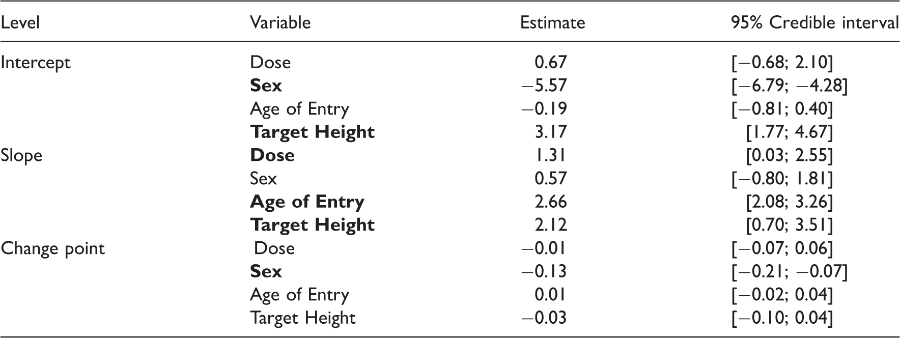
4.1 Parameter estimates

Parameter estimates (posterior means) and 95% credible intervals for the parameters of model 1 are presented in Table 1. To aid interpretation the coefficients are printed in bold whenever the credible interval includes 0. The dose has a positive effect on the speed of growth; however, the adult height was not significantly different. Quite remarkably, the children that start the therapy at a later age showed a faster growth and seemed to arrive at a comparable adult height as children that start earlier. This might indicate that the timing of the start of the growth hormone therapy is not critical. As we expected, boys attained their adult height later and also became taller. Children with a higher target height grew faster and tended to become taller.

Table 1.

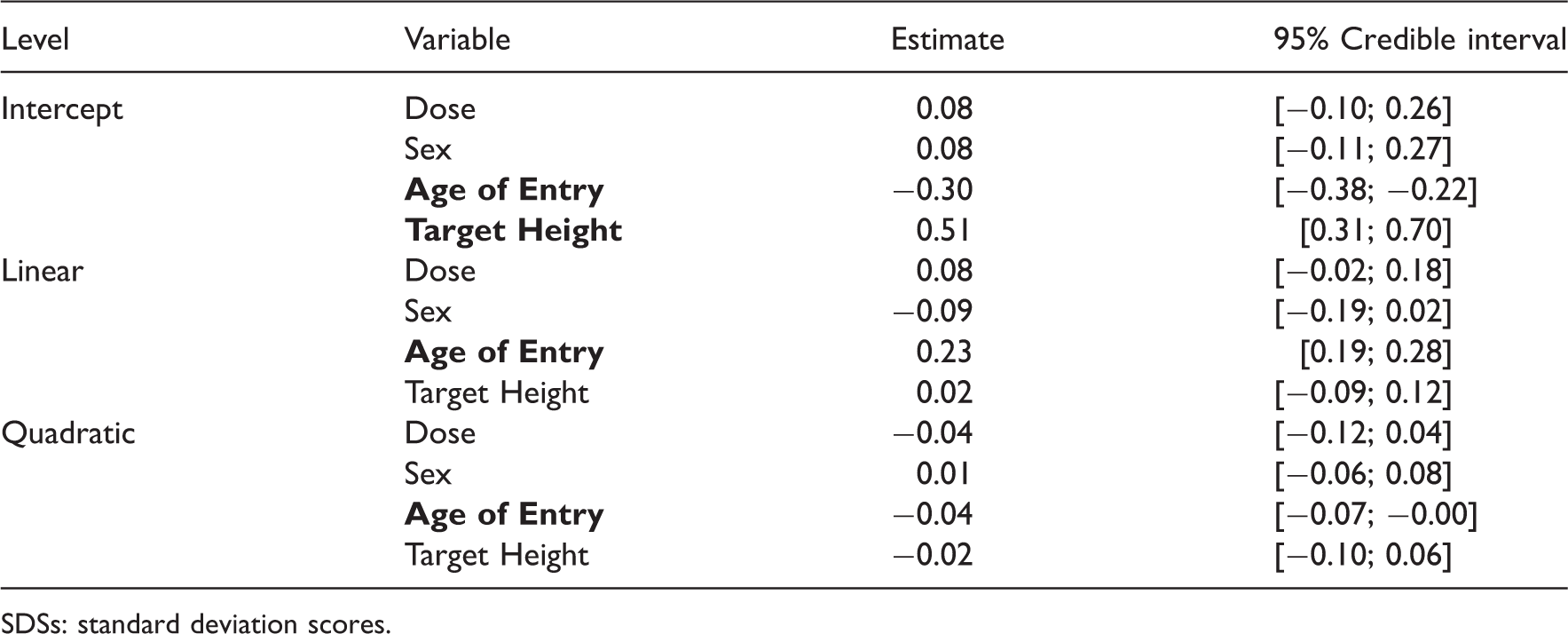
Estimated coefficients and associated credible intervals for the model of the untransformed height scores (sex is coded −1 for boys and 1 for girls, Dose as −1 for the low dose and 1 for a high dose).

Level	Variable	Estimate	95% Credible interval
Intercept	Dose	0.67	[−0.68; 2.10]
	Sex	−5.57	[−6.79; −4.28]
	Age of Entry	−0.19	[−0.81; 0.40]
	Target Height	3.17	[1.77; 4.67]
Slope	Dose	1.31	[0.03; 2.55]
	Sex	0.57	[−0.80; 1.81]
	Age of Entry	2.66	[2.08; 3.26]
	Target Height	2.12	[0.70; 3.51]
Change point	Dose	−0.01	[−0.07; 0.06]
	Sex	−0.13	[−0.21; −0.07]
	Age of Entry	0.01	[−0.02; 0.04]
	Target Height	−0.03	[−0.10; 0.04]

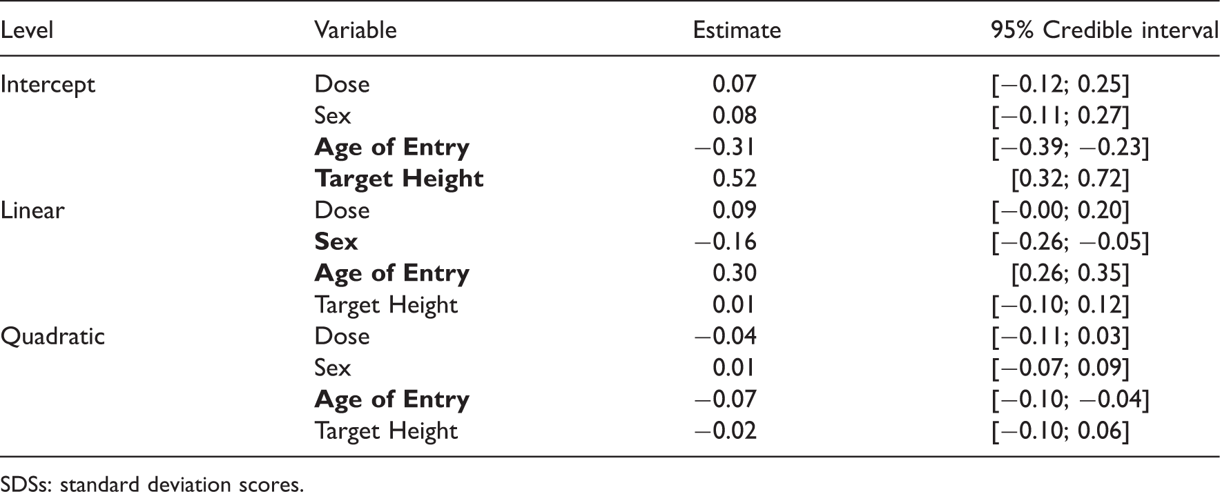
The parameter estimates and credible intervals for model 2 without a spline is presented in Table 2 and those with eight interior knots are presented in Table 3. Here it is more difficult to attribute a clear meaning to the individual coefficients. Because we were mainly interested in the effect of the growth hormone dose, we computed the effect of dose as a function of age (see the left panel of Figure 3). In principle such plots could also have been made for the other covariates but here we omitted this because of lack of space. From a similar plot for the starting age we learned that a later starting age leads to results that are just as good as when therapy is started early as the children grow faster.

Figure 3.

Average profiles for model 2. (a) Average profile for model 2 with 9 knots for boys with dose and age of entry set at zero and (b) average profile for model 2 with various numbers of knots with dose and age of entry set at zero.

Table 2.

Estimated coefficients and associated credible intervals for the model of the height SDSs without a spline (sex is coded −1 for boys and 1 for girls, Dose as −1 for the low dose and 1 for a high dose).

Level	Variable	Estimate	95% Credible interval
Intercept	Dose	0.08	[−0.10; 0.26]
	Sex	0.08	[−0.11; 0.27]
	Age of Entry	−0.30	[−0.38; −0.22]
	Target Height	0.51	[0.31; 0.70]
Linear	Dose	0.08	[−0.02; 0.18]
	Sex	−0.09	[−0.19; 0.02]
	Age of Entry	0.23	[0.19; 0.28]
	Target Height	0.02	[−0.09; 0.12]
Quadratic	Dose	−0.04	[−0.12; 0.04]
	Sex	0.01	[−0.06; 0.08]
	Age of Entry	−0.04	[−0.07; −0.00]
	Target Height	−0.02	[−0.10; 0.06]

SDSs: standard deviation scores.

Table 3.

Estimated coefficients and associated credible intervals for the model of the height SDSs with a spline with 9 knots.

Level	Variable	Estimate	95% Credible interval
Intercept	Dose	0.07	[−0.12; 0.25]
	Sex	0.08	[−0.11; 0.27]
	Age of Entry	−0.31	[−0.39; −0.23]
	Target Height	0.52	[0.32; 0.72]
Linear	Dose	0.09	[−0.00; 0.20]
	Sex	−0.16	[−0.26; −0.05]
	Age of Entry	0.30	[0.26; 0.35]
	Target Height	0.01	[−0.10; 0.12]
Quadratic	Dose	−0.04	[−0.11; 0.03]
	Sex	0.01	[−0.07; 0.09]
	Age of Entry	−0.07	[−0.10; −0.04]
	Target Height	−0.02	[−0.10; 0.06]

SDSs: standard deviation scores.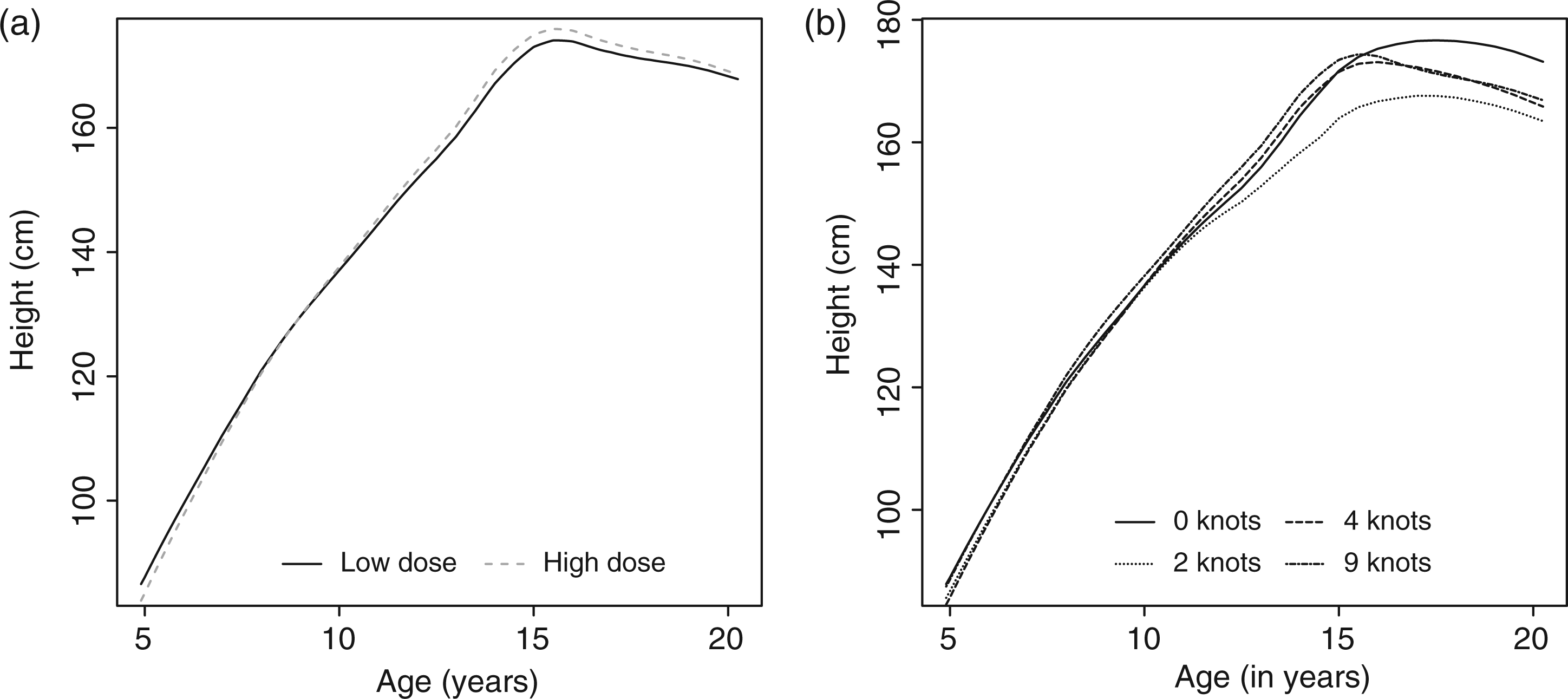

The addition of increasingly more knots to the spline allows a more complex relation between age SDS and height to be fit. In the right panel of Figure 3 we show how the inclusion of more knots to the model changes the average profile.

4.2 Comparing goodness of fit

The DIC (smaller is better) of model 1 converted to the SDS scale was −1 831. For the basic SDS model, i.e. without interior nodes, the DIC was 110. This value can be improved upon by adding nodes to the spline as can be seen from Table 4. It is clear from this table that model 1 always provides a much better fit to the data than model 2 even when a substantial number of nodes are added to the spline.

Table 4.

DIC (lower is better) of the untransformed height model compared with the model of the height SDS model with various numbers of interior knots.

Model of untransformed height		Model of height SDS
Effective df	DIC	Interior knots	Effective df	DIC
220.2	−1 831	0	224.0	110
		1	226.6	5
		2	228.1	−465
		3	229.7	−740
		4	230.6	−751
		5	232.6	−736
		6	233.3	−787
		7	233.2	−806
		8	234.3	−813
		9	235.2	−822

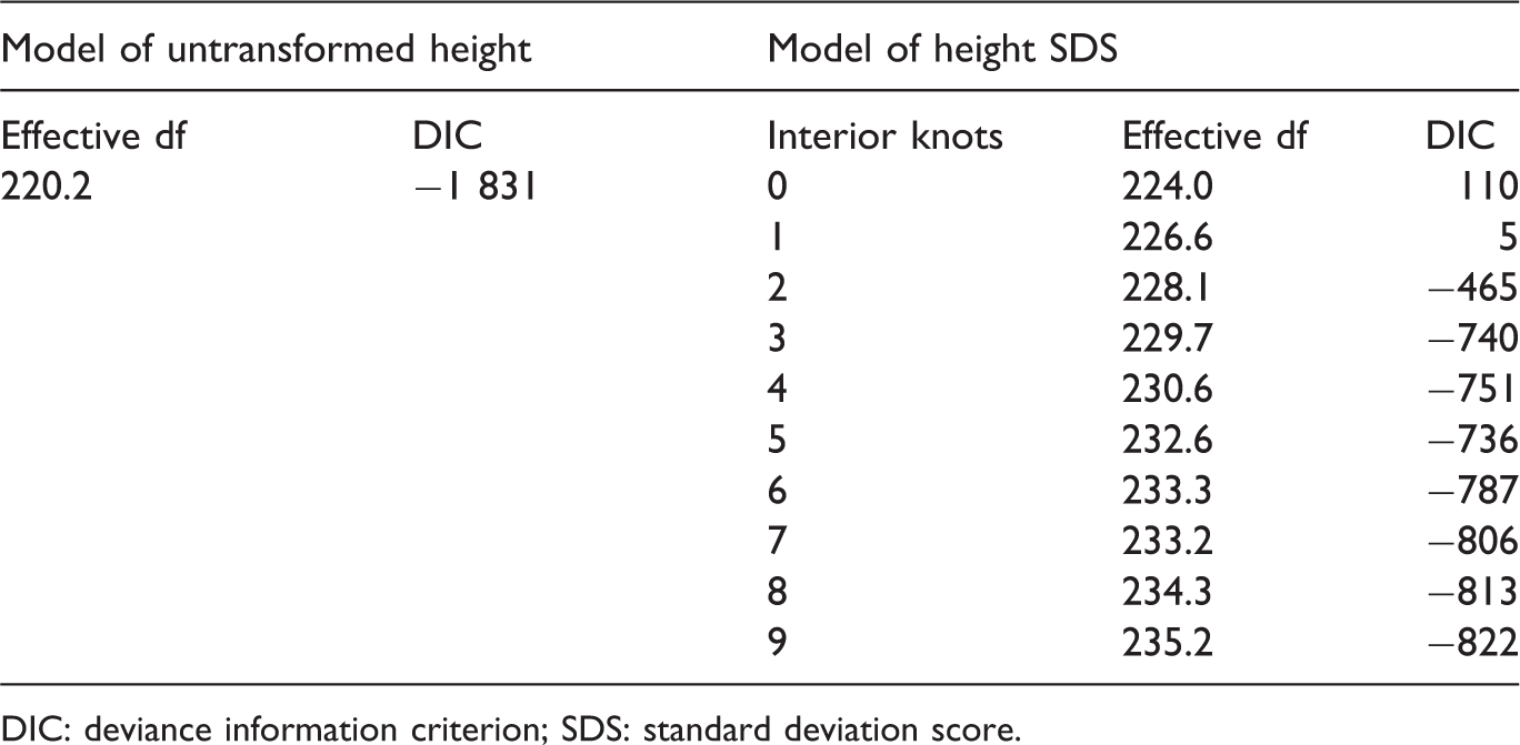
DIC: deviance information criterion; SDS: standard deviation score.

Based on graphical model diagnostics (not shown) we conclude that the assumptions of our model are reasonable. From the QQ-plots we saw that the assumptions of normality for the subject specific effects and measurement errors hold approximately. When the residuals were plotted against age, we saw that model 1 seemed to fit quite well overall. However, the variance seems to be larger at early ages. In addition at later ages the model seems to yield predictions that are slightly too low on average. There seemed to be a pattern in the residuals when no knots are in model 2. For model 2 involving splines there where no patterns in residuals. We could extend the models to incorporate non-normality and heteroskedasticity of the response in our model. However, we do not pursue this route here as it would distract from the main message.

4.3 Predictive ability

The RMSE of adult height for model 1 was 6.9 cm. For model 2 with 9 knots the RMSE evaluated at 20 years was 8.9 cm. So it appears that model 1 performs better than model 2. However, because the height does not remain constant after a certain age in model 2, for the RMSE depends at the age on which it is evaluated, when an other age than 20 is chosen the RMSE can be larger or smaller. In contrast in model 1 the adult height and hence the RMSE is clearly defined. Looking at the predicted profiles (Figure 4) we see that in model 2 it is very difficult to predict the change point correctly. In model 2 the predicted profiles are often downward sloping for certain age ranges, which is biologically impossible.

Figure 4.

Crossvalidated predicted profiles for selected individuals on the cm scale (0=observed, solid = model 1, dashed = model 2 using 9 knots).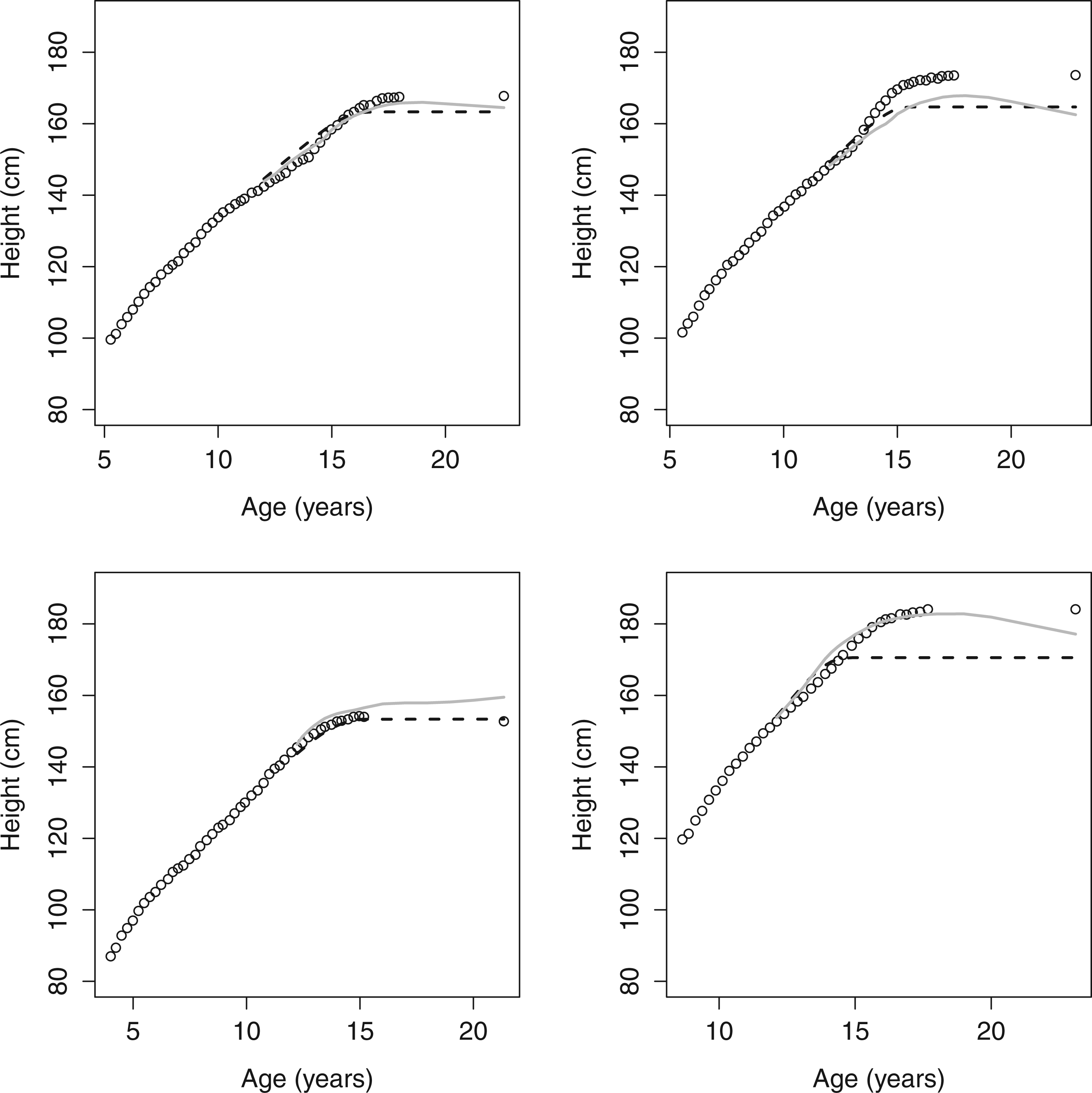

5 Discussion

Often mixed models are used to fit growth curves. Especially in endocrinology it is customary to do this on the SDS scale. The structure of these models can be quite complicated. Using the data from the DGH trial we saw that modeling on the original scale was much easier than on the SDS scale. We obtained a good fit using less parameters than when working on the SDS scale and with parameters that are easy to interpret.

It was shown that in our data set that the fit (expressed as the DIC) is better when we modeled height directly. This is because the structure of the model gets complicated when we transform the outcome to SDS scale for reasons that the studied group of children shows a different growth pattern than the reference population. When predicting adult height the predictions from the model on the SDS scale depend on the age at which we evaluate adult height. Furthermore, some of the predicted growth profiles were downward sloping when transformed to centimeters. Note that the models used give relatively low weight to the adult height because once a child reaches its adult height it is not measured anymore. When we would increase the weight of the last measurements, for example by including pseudo observations equal to the last recorded measurement, the model on the original scale performed better in prediction.

While there are some advantages to working with the SDS, in this article we provide a cautionary note to this standard practice. Depending on the research question and the group being investigated it depends whether modeling should be done on the original scale or on the SDS scale. When we want to make a comparison with a reference group or compare children across different ages, using the SDS scale has clear advantages making direct comparisons possible without additional corrections for age and sex. However, in randomized clinical trials where we want to compare between two treatment groups that are comparable in age and sex distribution modeling on the original scale can lead to simpler models. This is especially true if the population being investigated is different than the reference population or for ages around puberty where the SDS is difficult to interpret.

Footnotes

Funding

The author(s) received no financial support for the research and/or authorship of this article.

References

de Zegher

Ong

Ibez

. Growth hormone therapy in short children born small for gestational age. Horm Res 2006; 65(Suppl 3): 145–152.

Hokken-Koelega

de Waal

Sas

. Small for gestational age (SGA): endocrine and metabolic consequences and effects of growth hormone treatment. J Pediatr Endocrinol Metab 2004; 17(Suppl 3): 463–469.

Kamboj

. Short stature and growth hormone. Indian J Pediatr 2005; 72(2): 149–157.

Allen

. Growth hormone therapy for short stature: is the benefit worth the burden?. Pediatrics 2006; 118(1): 343–348.

Boguszewski

Albertsson-Wikland

Aronsson

. Growth hormone treatment of short children born small-for-gestational-age: the nordic multicentre trial. Acta Paediatr 1998; 87(3): 257–263.

Cooper

Eriksson

Forsn

. Maternal height, childhood growth and risk of hip fracture in later life: a longitudinal study. Osteoporos Int 2001; 12(8): 623–629.

Dalton

Rue

Silverman

. Height and weight in children treated for acute lymphoblastic leukemia: relationship to cns treatment. J Clin Oncol 2003; 21(15): 2953–2960.

de Zegher

Albertsson-Wikland

Wollmann

. Growth hormone treatment of short children born small for gestational age: growth responses with continuous and discontinuous regimens over 6 years. J Clin Endocrinol Metab 2000; 85(8): 2816–2821.

Hypponen

Virtanen

Kenward

. Obesity, increased linear growth, and risk of type 1 diabetes in children. Diab Care 2000; 23(12): 1755–1760.

10.

Kamp

Waelkens

de Muinck Keizer-Schrama

. High dose growth hormone treatment induces acceleration of skeletal maturation and an earlier onset of puberty in children with idiopathic short stature. Arch Dis Child 2002; 87(3): 215–220.

11.

Karaolis-Danckert

Buyken

Bolzenius

. Rapid growth among term children whose birth weight was appropriate for gestational age has a longer lasting effect on body fat percentage than on body mass index. Am J Clin Nutr 2006; 84(6): 1449–1455.

12.

Kjaergaard

Mller

Skovby

. Prepubertal growth in congenital disorder of glycosylation type ia (cdg-ia). Arch Dis Child 2002; 87(4): 324–327.

13.

Nguyen

Allen

Peat

. Growth and feeding practices of vietnamese infants in australia. Eur J Clin Nutr 2004; 58(2): 356–362.

14.

Ong

Preece

Emmett

. Size at birth and early childhood growth in relation to maternal smoking, parity and infant breast-feeding: longitudinal birth cohort study and analysis. Pediatr Res 2002; 52(6): 863–867.

15.

Rotteveel

van Weissenbruch

Twisk

. Infant and childhood growth patterns, insulin sensitivity, and blood pressure in prematurely born young adults. Pediatrics 2008; 122(2): 313–321.

16.

Davenport

Punyasavatsut

Stewart

. Growth failure in early life: an important manifestation of turner syndrome. Horm Res 2002; 57(5–6): 157–164.

17.

Bakker

Oostdijk

Geskus

. Patterns of growth and body proportions after total-body irradiation and hematopoietic stem cell transplantation during childhood. Pediatr Res 2006; 59(2): 259–264.

18.

Zemel

Kawchak

Fung

. Effect of zinc supplementation on growth and body composition in children with sickle cell disease. Am J Clin Nutr 2002; 75(2): 300–307.

19.

Cole

Green

. Smoothing reference centile curves: the lms method and penalized likelihood. Stat Med 1992; 11(10): 1305–1319.

20.

Wright

Royston

. Calculating reference intervals for laboratory measurements. Stat Meth Med Res 1999; 8(2): 93–112.

21.

Fredriks

Van Buuren

Burgmeijer

. Continuing positive secular growth change in the Netherlands 1955–1997. Pediatr Res 2000; 47(3): 316–323.

22.

van Wieringen

Verbrugge

. Growth diagrams of infants. a national survey, 1964–1966. Maandschr Kindergeneeskd 1966; 34(12): 389–414.

23.

Foulkes

Davies

. An index of tracking for longitudinal data. Biometrics 1981; 37(3): 439–446.

24.

Sas

de Waal

Mulder

. Growth hormone treatment in children with short stature born small for gestational age: 5-year results of a randomized, double-blind, dose-response trial. J Clin Endocrinol Metab 1999; 84(9): 3064–3070.

25.

van Pareren

Mulder

Houdijk

. Adult height after long-term, continuous growth hormone (gh) treatment in short children born small for gestational age: results of a randomized, double-blind, dose-response gh trial. J Clin Endocrinol Metab 2003; 88(8): 3584–3590.

26.

Johnston

Savage

. Should recombinant human growth hormone therapy be used in short small for gestational age children?. Arch Dis Child 2004; 89(8): 740–744.

27.

Hokken-Koelinga

de Ridder

Lemmen

. Children born small for gestational age: Do they catch up?. Pedeatr Res 1995; 38(2): 267–271.

28.

Lee

Chernausek

Hokken-Koelenga

Czernichow

. International small for gestational age advisory board consensus development conference statement: Management of short children born small for gestational age. Pedeatrics 2003; 111(6): 1253–1261.

29.

Roede

Van Wieringen

. Growth diagrams 1980, netherlands. third nation-wide survey. T Soc Gezondheidsz 1985; 63(Suppl): 1–34.

30.

Gilks

Roberts

Markov chain Monte Carlo in Practice Boca Roton: Chapman & Hall/CRC,1996.

31.

Ruppert

Wand

Carroll

Semiparametric regression Cambridge University Press, 2003.

32.

Spiegelhalter

Best

Carlin

. Bayesian measures of model complexity and fit. J Roy Stat Soc Ser B 2002; 64: 583–639.

33.

Spiegelhalter D, Thomas A, Best N and Lunn D. WinBUGS user manual version 1.4 2003.

34.

Gelman

Rubin

. Inference from iterative simulation using multiple sequences. Stat Sci 1992; 7: 457–511.