Binomial confidence intervals for testing non-inferiority or superiority: a practitioner’s dilemma

Abstract

In testing for non-inferiority or superiority in a single arm study, the confidence interval of a single binomial proportion is frequently used. A number of such intervals are proposed in the literature and implemented in standard software packages. Unfortunately, use of different intervals leads to conflicting conclusions. Practitioners thus face a serious dilemma in deciding which one to depend on. Is there a way to resolve this dilemma? We address this question by investigating the performances of ten commonly used intervals of a single binomial proportion, in the light of two criteria, viz., coverage and expected length of the interval.

Keywords

coverage expected length non-inferiority superiority

1 Introduction

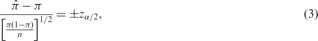
In biomedical research, the confidence interval (CI) of a single binomial proportion is frequently used in testing for non-inferiority or superiority. The typical one-sided hypothesis-testing formulation for non-inferiority is

H_{0} : π - π_{0} \leq - δ versus H_{1} : π - π_{0} > - δ

and for superiority is

H_{0} : π - π_{0} \leq δ versus H_{1} : π - π_{0} > δ

where

π_{0}

is the pre-specified probability and

δ (\geq 0)

is the margin (see Chow et al.¹ for further details).

To carry out a test for non-inferiority (superiority), practitioners often use available statistical packages to compute an appropriate CI of a binomial proportion. Incidentally, almost all statistical packages provide more than one option to compute a CI for a single binomial proportion. For example, the current version of SAS 9.3 (The SAS Institute, Cary, NC) offers six different intervals, Stata (Stata Corp LP, College Station, TX, USA) offers five different intervals, and SPSS (SPSS Inc, IL) offers three different intervals. The consequences of too many available choices are that, inferences drawn from different intervals often lead to conflicting conclusions. Thus, the practitioners are pushed to a situation requiring them to make an informed choice.

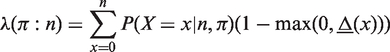
To illustrate a similar situation we consider a recent post-market urology study; 31 patients were treated with a medical device for their stress urinary incontinence syndrome, where older women are unable to hold their urine, and it leaks due to minor physical activities like coughing, walking, etc. After 12 months, 28 patients reported the efficacy of the treatment, and three of them reported a worsened status. Based on the historical success rate of 85% for other devices already available in the market, the study was intended to check the non-inferiority of the device, with a 10% margin. Therefore, the null hypothesis $H_{0} : π \leq 0.75$ was tested against the alternative $H_{1} : π > 0.75$ . With n = 31 and x = 28, the following 95% confidence intervals were obtained using SAS 9.3 software and R code stated later in this paper.

Since the “use of the standard textbook method

x / n \pm 1.96 \sqrt{((x / n) (1 - x / n) / n)}

, or its continuity corrected version, are strongly discouraged” (Vollset²), we do not report them here. Notice that (cf. Table 1) five of the intervals lead to the rejection of the null hypothesis while the other four do not.

Table 1.

Two-sided 95% confidence intervals of the results of device study.

Methods	Lower CL	Upper CL	P
SOC^a	0.763	0.974	$< 0.025$
JF	0.764	0.972	$< 0.025$
AC	0.743	0.974	$> 0.025$
SCC	0.749	0.967	$> 0.025$
SC	0.751	0.967	$< 0.025$
BS	0.755	0.973	$< 0.025$
BL	0.749	0.973	$> 0.025$
MCP	0.759	0.975	$< 0.025$
CP^a	0.743	0.98	$> 0.025$

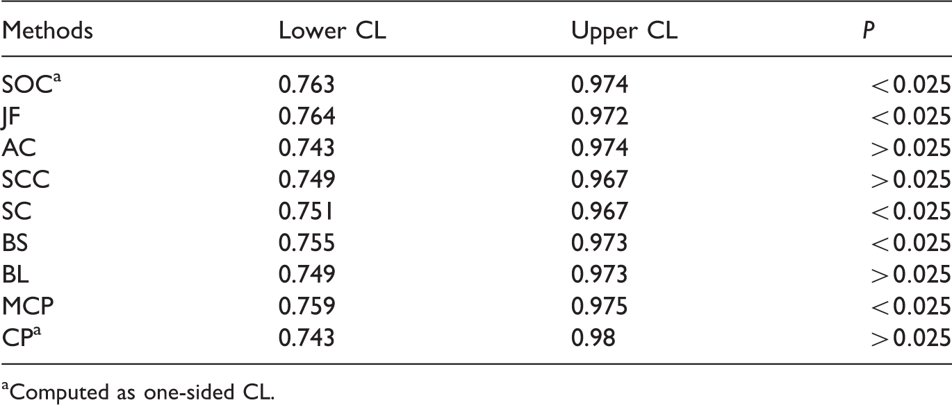
Computed as one-sided CL.

We address this issue by comparing the performances of the often used CIs based on two criteria, viz. coverage and expected length. Newcombe^3–5 compared the performances of seven two-sided confidence intervals of a single binomial proportion. Unlike Newcombe, in this paper we address the problem of testing non-inferiority (superiority) using a confidence interval approach. Thus our focus is on studying the performance of one-sided CIs. Cai⁶ considers the problem of finding a one-sided CI of the parameter μ of the natural exponential family with a quadratic variance function (NEF-QVF). This family of distributions in particular includes binomial distribution as a special case. However, unlike ours, the primary focus of his study was to derive a second-order corrected one-sided CI (SOC) of μ using the Edgeworth expansion of the coverage probability. We consider SOC in our data analysis and compare its performance with others. Also, unlike Newcombe^3,4 we consider a few more exact intervals besides the standard asymptotic intervals. The primary reason for considering the exact intervals is that the asymptotic intervals may not attain the nominal coverage, which Corcoran and Mehta⁷ and Casella⁸ found undesirable. Borkowf⁹ states, “sine qua non of CI construction is nominal coverage. A confidence procedure must provide nominal coverage (near) to be valuable, and then one can focus on secondary aspects, such as minimizing the mean interval widths …” Incidentally, however, some of the one-sided CI’s computed from exact two-sided CIs may fail to attain nominal coverage. Thus, the above argument for using exact CIs is no longer tenable for testing non-inferiority (superiority) without investigating its coverage property. In our practical experience, however, we have seen that practitioners often miss out on this subtle fact. They often presume that nominal coverage is guaranteed for a one-sided CI, since it is based on an exact two-sided CI.

There are statisticians who question the legitimacy of taking up an inflexible stance on attaining nominal coverage as stated above. Brown et al.¹⁰ (BCD) in an important paper suggested that one should instead consider a trade-off between the coverage and the precision (expected length) for comparing different intervals. Following BCD recently, Newcombe and Nurminen¹¹ have come up with an interesting idea that “in the evaluation of various methods it is more appropriate to consider the moving average of the coverage probabilities” over an interval of parameter values, instead of sticking to the requirement of nominal coverage probabilities. But, in this paper, we refrain from entering into the philosophical debate of coverage versus precision, and the trade-off thereof that one could look for. We would rather keep the option open for the practitioners to decide what suits them best in a given situation.

Another good reason for considering exact CIs is that, with the availability of high-speed computers, exact intervals are now easily computable for any reasonable sample size and thus have become quite popular among the practitioners. In fact, these intervals are now available in standard statistical packages; for example, the Clopper–Pearson interval (CP) is available in SAS, StatXact, R, and S-Plus; the Blyth-Still-Casella interval (BS) is available in StatXact; and the interval due to Blaker (BL) and the mid-p adjusted Clopper–Pearson interval (MCP) are available in R.

In this article, we compare five asymptotic intervals – Wald with continuity correction (AS) (Fleiss et al.¹²), Wilson (SC),¹³ Wilson with continuity correction (SCC) (Fleiss et al.¹²), Agresti-Coull (AC),¹⁴ and second-order corrected (SOC) one-sided CI (Cai⁶); a Bayesian interval using Jeffreys’ prior (JF) (Brown et al.¹⁰); and four exact intervals – Clopper–Pearson¹⁵ (CP), mid-p adjusted Clopper–Pearson (MCP), Blaker (BL),¹⁶ and Blyth-Still-Casella (BS) (Blyth and Still,¹⁷ Casella¹⁸). The use of the continuity-corrected Wald interval (AS) is strongly discouraged for its poor coverage property (Vollset²). However, we decided to include it in discussion for the sake of completeness, since it is available in all standard statistical packages (for example SAS’s PROC FREQ).

In Section 2, we briefly describe the methods of finding the above confidence intervals. Section 3 presents an extensive simulation study comparing the intervals in terms of coverage and expected length. In Section 4, we present our case with a real-life dataset, and finally, in Section 5 we give the concluding discussion.

2 Confidence intervals

We consider intervals of three types viz., Asymptotic, Bayesian and Exact, depending on the methodology being used for finding them. Suppose X denotes the number of successes in n independent Bernoulli trials with constant probability of success π. Given x, the observed value of X, we denote the observed success rate $\frac{x}{n}$ by $\overset{\land}{π}$ . We also denote the lower and upper limits of the confidence interval of π by $\underline{Δ} (x)$ and $\bar{Δ} (x)$ , respectively. From a $100 (1 - α) %$ two-sided CI, a $100 (1 - α / 2) %$ one-sided CI is obtained by considering either $(max (0, \underline{Δ} (x)), 1)$ or $(0, min (1, \bar{Δ} (x))$ . It needs mentioning that the Clopper–Pearson intervals are specifically derived from one-sided CIs. This is precisely the reason why it guarantees at least nominal coverage for both two-sided and one-sided CI’s. Except for the Clopper–Pearson interval, all one-sided intervals are obtained from the corresponding two-sided intervals. Also, it is worthwhile to mention here that, all CIs considered here have equi-variance property – viz., the limits of the CI based on $(n - x) / n$ are complements of those based on x/n.

2.1 Asymptotic intervals

2.1.1 AS: asymptotic Wald interval with continuity correction

This is a continuity-corrected Wald interval given in Fleiss et al.¹² The Wald interval is obtained by inverting the Wald test for π and is given by

\overset{\land}{π} \pm z_{α / 2} \sqrt{\overset{\land}{π} (1 - \overset{\land}{π}) / n}

(1)

The continuity-corrected interval uses the following formula:

\overset{\land}{π} \pm z_{α / 2} \sqrt{\overset{\land}{π} (1 - \overset{\land}{π}) / n} + 1 / (2 n)

(2)

where

z_{α / 2}

is the

100 (1 - α / 2)

-th percentile of the standard normal distribution.

2.1.2 SC: Score interval (Wilson¹³)

The CI based on the score statistic was first proposed by Edwin B. Wilson.¹³ Setting the score statistic equal to the critical z values,

\frac{\overset{\land}{π} - π}{[\frac{π (1 - π)}{n}] 1 / 2} = \pm z_{α / 2},

(3)

the endpoints of the interval are obtained as solutions to a quadratic equation in π and have the following form

w \overset{\land}{π} + \frac{1}{2} (1 - w) \pm z_{α / 2} [w 2 \frac{\overset{\land}{π} (1 - \overset{\land}{π})}{n} + (1 - w) 2 \frac{(1 / 2) (1 / 2)}{z_{α / 2}^{2}}] 1 / 2

(4)

where

w = n / (n + z_{α / 2}^{2})

. The interval is known as Wilson’s score interval, or in short, the score interval. Notice that the centre of the interval is a weighted average of the observed success rate

\overset{\land}{π}

and 1/2, and it approaches

\overset{\land}{π}

with increasing value of n or decreasing value of

z_{α / 2}

. We may also consider the centre as the average resulting from an a priori random experiment with outcomes 1/2 and

\overset{\land}{π}

having probabilities of occurrences proportional to

z_{α / 2}^{2}

and n respectively. If w is fixed, the empirical standard error of the centre computed from this experiment is exactly the same as that given in equation (4).

It is a frequently used CI in many applications, especially in biomedical research, since it is known to have good coverage properties with shorter length. Both Newcombe³ and BCD¹⁰ recommend this interval.

2.1.3 SCC: score interval with continuity correction

The continuity-corrected version of the score interval is obtained by replacing $\overset{\land}{π}$ in equation (4) by $\overset{\land}{π} * = \overset{\land}{π} + 1 / (2 n)$ for the upper limit and $\overset{\land}{π} * = \overset{\land}{π} - 1 / (2 n)$ for the lower limit:

w \overset{\land}{π} * + \frac{1}{2} (1 - w) \pm z_{α / 2} [w 2 \frac{\overset{\land}{π} * (1 - \overset{\land}{π} *)}{n} + (1 - w) 2 \frac{(1 / 2) (1 / 2)}{z_{α / 2}^{2}}] 1 / 2

(5)

\overset{\land}{π}

is 0 or 1, then the lower or upper bound is fixed at 0 or 1, respectively.

2.1.4 AC: Agresti–Coull interval

An asymptotic interval proposed by Agresti and Coull¹⁴ is based on a simple adjustment of the Wald interval obtained by adding “two successes and two failures” to the sample when the nominal coverage probability is 0.95. Therefore, the point estimate is ${\overset{\land}{π}}_{adj} = \frac{x + 2}{n + 4}$ . This is approximately equal to $(x + \frac{1}{2} z_{α / 2}^{2}) / (n + z_{α / 2}^{2})$ when $α = 0.05$ , and the resulting confidence interval is

{\overset{\land}{π}}_{adj} \pm z_{α / 2} \sqrt{{\overset{\land}{π}}_{adj} (1 - {\overset{\land}{π}}_{adj}) / (n + 4)} .

(6)

BCD¹⁰ recommended this interval based on their study.

2.1.5 SOC: Second order corrected interval

Cai⁶ proposes a one-sided asymptotic CI by removing the first and second-order systematic bias terms from the coverage based on its Edgeworth expansion. The resulting one-sided CIs with $100 (1 - α) %$ coverage are obtained as:

[0, \tilde{π} + z_{α} (V (\overset{\land}{π}) + (γ_{1} V (\overset{\land}{π}) + γ_{2}) n - 1) 1 / 2 n - 1 / 2]

(7)

[\tilde{π} - z_{α} (V (\overset{\land}{π}) + (γ_{1} V (\overset{\land}{π}) + γ_{2}) n - 1) 1 / 2 n - 1 / 2, 1]

(8)

where

η = (z_{α}^{2} / 3 + 1 / 6), γ_{1} = - (13 z_{α}^{2} / 18 + 17 / 18), γ_{2} = (z_{α}^{2} / 18 + 7 / 36)

and

\tilde{π} = (x + η) / (n + 2 η) .

For further details we refer to Cai.⁶

2.2 Bayesian interval

2.2.1 JF: Jeffreys’ prior interval

This is an equal-tailed posterior probability interval using Jeffreys noninformative prior which is Beta(1/2,1/2) having density $f (π) \propto π - 1 / 2 (1 - π) - 1 / 2, 0 < π < 1$ . The resulting limits of the posterior probability interval with posterior probability $1 - α$ are:

\underline{Δ} (x) = B (α / 2; x + 1 / 2, n - x + 1 / 2)

\bar{Δ} (x) = B (1 - α / 2; x + 1 / 2, n - x + 1 / 2)

where

B (α, a, b)

denotes the α-th quantile of Beta(a, b) distribution. BCD¹⁰ recommended this interval.

2.3 Exact intervals

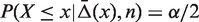
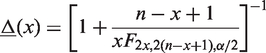
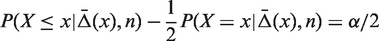
2.3.1 CP: Clopper–Pearson interval

The lower $\underline{Δ} (x)$ and upper $\bar{Δ} (x)$ limits of the Clopper–Pearson interval are obtained as solutions to the following equations:

P (X \geq x | \underline{Δ} (x), n) = α / 2

P (X \leq x | \bar{Δ} (x), n) = α / 2

where

\underline{Δ} (x) = 0

x = 0

, and

\bar{Δ} (x) = 1

x = n

. Alternatively, the limits can be obtained directly from the distribution (see Collett¹⁹, Leemis and Trivedi²⁰) as follows:

\underline{Δ} (x) = [1 + \frac{n - x + 1}{{xF}_{2 x, 2 (n - x + 1), α / 2}}] - 1

\bar{Δ} (x) = [1 + \frac{n - x}{(x + 1) F_{2 (x + 1), 2 (n - x), 1 - α / 2}}] - 1

where

F_{n, m, α}

represents the upper

100 α

percentile point of the F-distribution with n and m degrees of freedom. As before we have,

\underline{Δ} (x) = 0

x = 0

, and

\bar{Δ} (x) = 1

x = n

. Notice that this two-sided interval is obtained from two one-sided intervals. For other intervals except MCP, it is the other way around.

2.3.2 MCP: Mid-P adjusted Clopper–Pearson interval

Exact intervals are known to be conservative, and consequently they are wider in length than their asymptotic counterparts. Agresti and Gottard²¹ revisited mid-p adjustment (Lancaster²²), Berry and Armitage,²³ Vollset,² Newcombe³) of the Clopper–Pearson interval. In the computation of the mid-P value, only 1/2 of the point probability 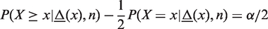$P (X = x | π, n)$ is counted instead of the whole. Thus, the lower limit $\underline{Δ} (x)$ and the upper limit $\bar{Δ} (x)$ of the mid-p adjusted Clopper–Pearson interval are obtained by solving the following equations:

P (X \geq x | \underline{Δ} (x), n) - \frac{1}{2} P (X = x | \underline{Δ} (x), n) = α / 2

P (X \leq x | \bar{Δ} (x), n) - \frac{1}{2} P (X = x | \bar{Δ} (x), n) = α / 2

where

\underline{Δ} (x) = 0

x = 0

, and

\bar{Δ} (x) = 1

x = n

. This interval is found to be less conservative than the Clopper–Pearson interval. Unfortunately, unlike CP this interval cannot be obtained in a closed form. In fact, it does not appear to be in the category of intervals which could be easily implemented in a spreadsheet.

2.3.3 BL: Blaker’s interval

This is a less popular CI, which is available in R and S-Plus. Blaker uses Spjøtvoll’s (Spjøtvoll,²⁴ Blaker and Spjøtvoll²⁵) notion of a preference function (PF) to improve upon the interval proposed by Birnbaum.²⁶ Birnbaum bases his interval on the P-value of the equal-tailed test of $H_{0} : π = π_{0}$ as follows.

Given $x, B_{α} (x) = {π : β (π; x) > α}$ is a CI with minimum coverage $1 - α$ , where $β (π; x) = min [2 min {P (X \geq x | π, n), P (X \leq x | π, n)}, 1]$ .

Note $β (π; x)$ represents the P-value of the equal-tailed test. Spjøtvoll defines PF $β (π; x)$ as a real-valued function on the parameter space for each observed x. Given a PF $β (π; x)$ and an observed x, the parameter value $π_{1}$ is preferable to $π_{2}$ if $β (π_{1}; x) > β (π_{2}; x)$ . Note that $β (π; x)$ given by Birnbaum is a PF and has the additional property that ${π : β (π; x) > α}$ is a $1 - α$ CI for π. Blaker, considers the PF $λ (π; x) = P {γ (π; X) \leq γ (π; x)}$ where $γ (π; x) = min {P (X \geq x), P (X \leq x)}$ and proves that the set $C_{α} (x) = {π : λ (π; x) > α}$ is a CI with minimum coverage $1 - α$ . Since $β (π; x) \geq λ (π; x)$ (cf. Blaker²⁵) for all x, the CI’s based on $λ (π; x)$ are shorter than the ones based on $β (π; x)$ and hence is an improvement over Birnbaum’s interval.

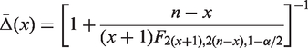
2.3.4 BS: Blyth-Still-Casella interval

This interval is available only in StatXact software. A confidence set of π, say C, is a collection of 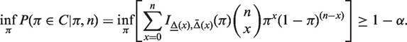$(n + 1)$ intervals, $(\underline{Δ} (x), \bar{Δ} (x)), x = 0, 1, \dots, n$ . The coverage of the confidence procedure is thus given by

{inf}_{π} P (π \in C | π, n) = {inf}_{π} [\sum_{x = 0}^{n} I_{\underline{Δ} (x), \bar{Δ} (x)} (π) (n x) π x (1 - π) (n - x)] \geq 1 - α .

The expression inside the parentheses represents the probability that the random interval 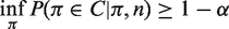$(\underline{Δ} (x), \bar{Δ} (x))$ contains the true parameter value π. Notice that if

{inf}_{π} P (π \in C | π, n) \geq 1 - α

for a specified minimum coverage

1 - α

, it is possible to construct a refined procedure

C * = {(\underline{Δ} * (x), \bar{Δ} * (x)); x = 0, 1, \dots, n

directly by increasing

\underline{Δ} (x)

\underline{Δ} * (x)

(and decreasing

\bar{Δ} (x)

by the same amount) starting from

x = n

until we reach

P (\underline{Δ} * (x) \in C | \underline{Δ} * (x), n) = 1 - α

for all x. Casella¹⁸ gives an algorithm to produce a collection of refined intervals with uniformly shorter length when applied to any

1 - α

binomial confidence procedure. The resulting confidence intervals have some optimal properties (Casella¹⁸). As noted by Newcombe⁴ (cf. Table 6), shortened intervals like Sterne’s²⁷ have erratic location properties. Consequently, its impact on the coverage of one-sided CI is worth exploring. Our simulation study (Section 3) clearly shows that the one-sided CI’s based on two-sided BL and BS intervals suffer from serious undercoverage even for very large sample sizes.

3 Simulation study

In this section, we discuss the results of an extensive simulation study. We consider sample sizes $n = 25, 50, 100, 1000$ . To find coverage and expected length of a CI we partition the parameter space [0, 1] into 10,000 equally spaced points. Each partition point corresponds to a value of π. For a one-sided interval of the form $(max (0, \underline{Δ} (x)), 1)$ the coverage probability and the expected length corresponding to a partition point π are computed by using the expressions:

ζ (π : n) = \sum_{x = 0}^{n} P (X = x | n, π) I (π \in (max (0, \underline{Δ} (x)), 1))

λ (π : n) = \sum_{x = 0}^{n} P (X = x | n, π) (1 - max (0, \underline{Δ} (x)))

Note coverage and expected length are functions of success probability π and sample size n. For a fixed sample size, the distributions of these entities could be found assuming a uniform distribution of π. We produce BliP plots (Lee and Tu²⁸) for representing these distributions pictorially. The vertical bars in each plot show the deciles of the corresponding distribution. For the coverage plot, a long vertical line is drawn at the 97.5% coverage.

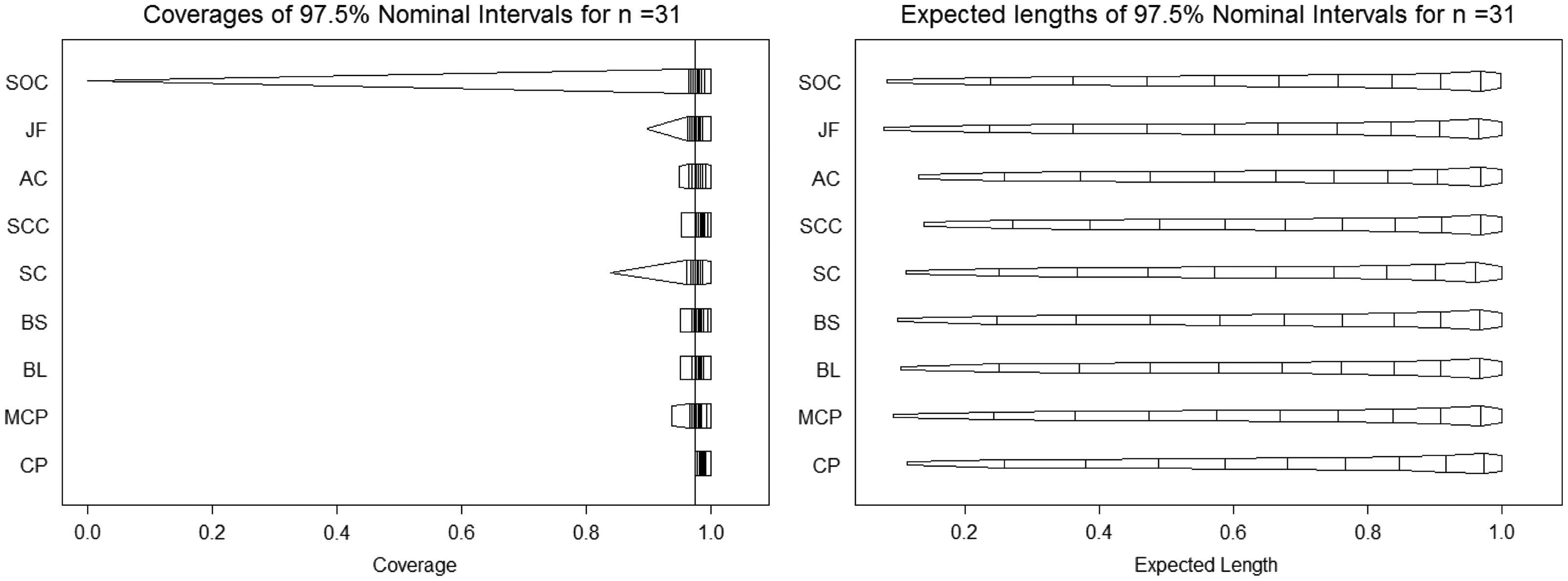
The BliP plots of coverage and expected length of all the intervals except AS and SOC are presented in Figure 1 for the sample sizes mentioned above. Blip plot for AS is not included since its performance as expected is way below the others. On the other hand for values of π near the boundaries the under-coverage of SOC interval is worse than Jeffreys’ (see Figure 2), though the overall coverage behaviour of SOC is slightly better than Jeffreys’. Thus inclusion of SOC interval in the Blip plot creates a scaling problem in the sense that the visual comparison of others becomes difficult. We draw the Blip plot of SOC interval (see Figure 2) while revisiting the example in Section 4. For moderately large sample sizes its performance is similar to Jeffreys’.

Figure 1.

Blip plot of 97.5% one-sided coverage and expected length for n = 25, 50, 100, 1000.

Figure 2.

Blip plot of one-sided 97.5% coverage and expected length for n = 31.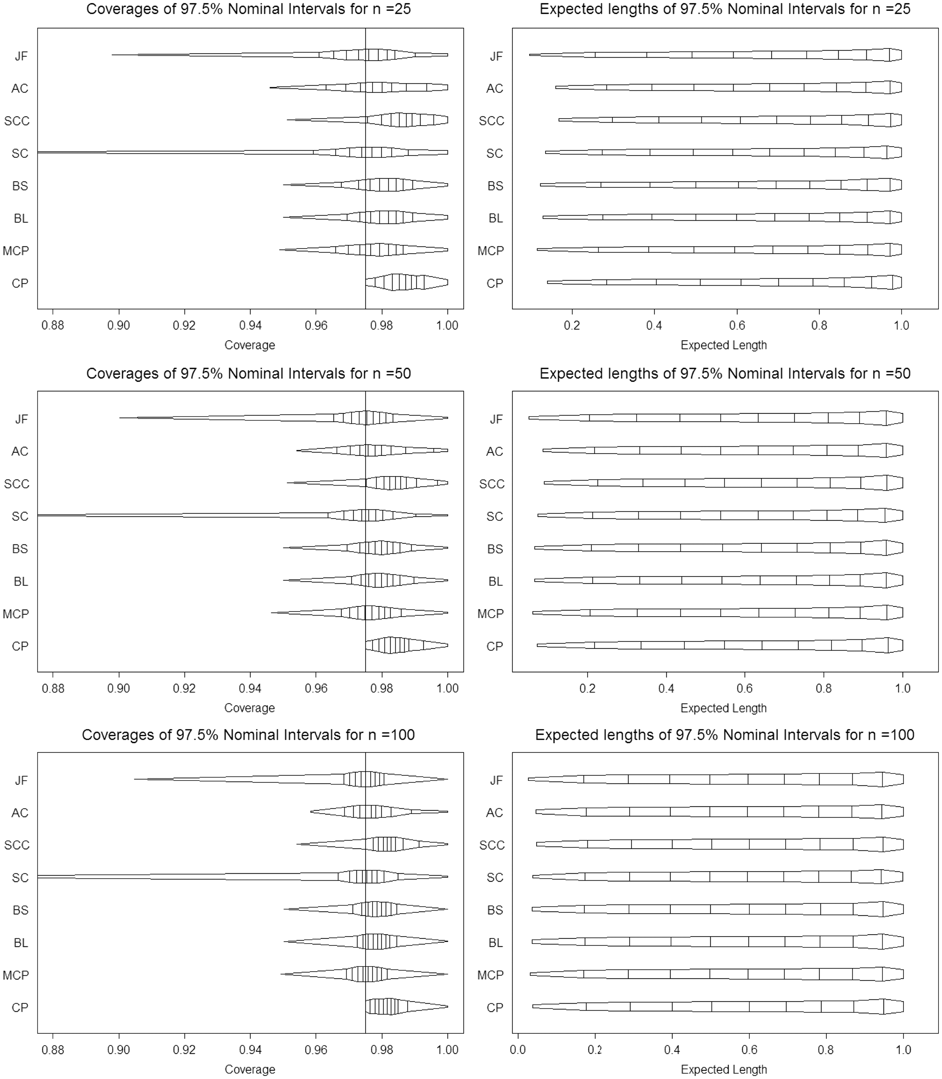

It is evident that from the standpoint of aligning minimum coverage with $1 - α$ all the asymptotic methods, except SCC, suffer from serious under coverage, with AS being the worst offender (though not shown in the figures). Among the exact intervals, except CP, all suffer from under coverage and MCP performs the worst. Note that, both BL and BS are, by construction, two-sided intervals and both, in order to reduce the expected length, result in intervals that have unequal non-coverage at the two ends. As a result, the one-sided CI obtained from these intervals may not attain the nominal coverage. MCP, of course, by construction, may not ensure the nominal coverage. On the other hand, CP being generated from two one-sided intervals, each of which ensures coverage $α / 2$ at both ends, it attains the nominal coverage. Notice that the two-sided intervals SC, and JF, recommended by either BCD¹⁰ or Newcombe,³ suffer from serious under-coverage even for very large sample sizes. SOC performs slightly better than JF with regard to the coverage except for the values of π near the boundaries. In the latter case, undercoverage could be substantial (not shown in Figure 1). It is true that the left tails of the expected length distribution of these CI’s are slightly more elongated than BL, AC and CP, in particular for small sample sizes. However, for sample sizes 100 and more, these differences become unnoticeable. But, as mentioned above, the coverage distributions of SC, JF and SOC show serious under-coverage, even for large sample sizes. If under-coverage is a serious concern, CP is clearly the choice. However, if we are ready to trade off a little with expected length, SCC comes next to CP since its under-coverage is around ten percent at the most and then comes BL, AC and BS.

4 Revisiting the example: stress urinary incontinence study

We revisit the example that we have considered in the beginning. We find this example useful for two reasons. First, it is about a study that was conducted. Secondly, it leads to conflicting inference. The intervals BL, AC, SCC, and CP do not reject the null hypothesis of non-inferiority, while the intervals JF, SOC, SC, AS, MCP, BS reject. In order to understand the phenomenon, we draw the blip plots of the CI’s for $n = 31$ (see Figure 2). Note that the left tails of the distribution of expected length of the intervals JF, SOC, SC, AS, MCP, BS are located to the left of BL, AC, SCC, and CP. Thus, there is a possibility that the lower limits of the former intervals are located to the right of the latter. Consequently, the value of 0.75 is not included in the former intervals but is included in the latter and hence leading to the rejection of null hypotheses by the former but not by the latter. Now the question is, should a practitioner reject or not reject the null hypothesis? We leave the decision to the practitioner.

5 Concluding remarks

This article is written primarily for two reasons. First, as practitioners, we often encounter a situation similar to the one presented in this paper. By conducting an extensive simulation study and drawing upon theoretical insights, we could explain why such a situation arises. Second, we reason that, if we understand why such a situation could arise, we are in a position to take an informed decision. We take an eclectic view on this matter and would not like to offer a solution. We leave it to the practitioner to decide depending on his or her own perspective. However, “there is a caveat”. Our study clearly shows that with increase in sample size the gain in expected length is clearly outweighed by loss in coverage.

We have noted at the outset that for testing inferiority practitioners prefer to use CI. One may wonder why a hypothesis test is not carried out directly instead of using CI for finding the P-value in an indirect way. The reason is, for some of the CIs (like SOC, BS and BL) finding the acceptance regions of the corresponding tests by inverting it is difficult although theoretically possible. Thus for these intervals a direct test of hypothesis is difficult to implement. On the other hand for intervals like AS, SC, AC and CP the hypothesis of inferiority could be easily tested directly.

Finally, we want to make a few remarks about the computation methods used. We have used StatXact to compute all confidence intervals for BS; to our knowledge StatXact is the only commercially available software to compute a confidence interval using BS method. For implementing Blaker’s interval, MCP, and a number of the asymptotic intervals, we used the R codes from Alan Agresti (http://www.stat.ufl.edu/ aa/cda/R/one-sample/R1/).

Footnotes

Acknowledgements

We thank Professor Newcombe and an anonymous referee for many useful comments that led to substantial improvement of the presentation of this article. We also thank Brian Johnson for his constructive comments on an early version of this manuscript.

Declaration of conflicting interests

The author(s) declared no potential conflicts of interest with respect to the research, authorship, and/or publication of this article.

Funding

The author(s) received no financial support for the research, authorship, and/or publication of this article.

References

Chow

Shao

Wang

. Sample size calculations in clinical research, Boca Raton, FL: CRC Press, 2003.

Vollset

. Confidence intervals for a binomial proportion. Stat Med 1993; 12: 809–824.

Newcombe

. Two-sided confidence intervals for the single proportion: comparison of seven methods. Stat Med 1998; 17: 857–872.

Newcombe

. Measures of location for confidence intervals for proportions. Commun Statist –Theory Methods 2011; 10: 1743–1767.

Newcombe

. Confidence intervals for proportions and related measures of effect size, Taylor & Francis: CRC Press, 2012.

Cai

. One-sided confidence intervals in discrete distributions. J Statist Plan Infer 2005; 131: 63–88.

Corcoran

Mehta

. Discussion of “Interval estimation for a binomial parameter” (by Lawrence Brown, T. Tony Cai and Anirban Das Gupta). Statist Sci 2001; 16: 122–124.

Casella

. Discussion of “Interval estimation for a binomial parameter” (by Lawrence Brown, T. Tony Cai and Anirban Das Gupta). Statist Sci 2001; 16: 120–122.

Borkowf

. Constructing binomial confidence intervals with near nominal coverage by adding a single imaginary failure or success. Stat Med 2006; 25: 3679–3695.

10.

Brown

Cai

DasGupta

. Confidence intervals for a binomial proportion (with discussion). Statist Sci 2001; 16: 101–133.

11.

Newcombe

Nurminen

. In defence of score intervals for proportions and their differences. Commun Statist –Theory Methods 2011; 40: 1271–1282.

12.

Fleiss

Levin

Paik

. Statistical methods for rates and proportions, 3rd ed. New York: John Wiley & Sons, Inc, 2003.

13.

Wilson

. Probable inference, the law of succession, and statistical inference. J Am Statist Assoc 1927; 22: 209–212.

14.

Agresti

Coull

. Approximate is better than “exact” for interval estimation of binomial proportions. Am Statist 1998; 52: 119–126.

15.

Clopper

Pearson

. The use of confidence or fiducial limits illustrated in the case of the binomial. Biometrika 1934; 26: 404–413.

16.

Blaker

. Confidence curves and improved exact confidence intervals for discrete distributions. Can J Statist 2000; 28: 783–798.

17.

Blyth

Still

. Binomial confidence intervals. J Am Statist Assoc 1983; 78: 108–116.

18.

Casella

. Refining binomial confidence intervals. Can J Statist 1986; 14: 113–129.

19.

Collett

. Modeling binary data, London: Chapman & Hall, 1991.

20.

Leemis

Trivedi

. A comparison of approximate interval estimators for the Bernoulli parameter. Am Statist 1996; 50: 63–68.

21.

Agresti

Gottard

. Nonconservative exact small-sample inference for discrete data. Comput Stat Data Anal 2007; 52: 6447–6458.

22.

Lancaster

. The derivation and partition of X² in certain discrete distributions. Biometrika 1949; 36: 117–129.

23.

Berry

Armitage

. Mid-p confidence intervals: a brief review. Statistician 1995; 44: 417–423.

24.

Spjøtvoll

Preference functions. In: Bickel

Doksum

Hodges

Jr (eds). A festschrift for Erich L. Lehmann, Belmont, CA: Wadsworth, 1983, pp. 409–432.

25.

Blaker

Spjøtvoll

. Paradoxes and improvements in interval estimation. The Am Statist 2000; 54: 242–247.

26.

Birnbaum

. Confidence curves: an omnibus technique for estimation and testing statistical hypotheses. J Am Statist Assoc 1961; 56: 246–249.

27.

Sterne

. Some remarks on confidence or fiducial limits. Biometrika 1954; 41: 275–278.

28.

Lee

. A versatile one-dimensional distribution plot: the BLiP plot. Am Statist 1997; 51: 353–358.

Binomial confidence intervals for testing non-inferiority or superiority: a practitioner’s dilemma

Abstract

Keywords

1 Introduction

2 Confidence intervals

2.1 Asymptotic intervals

2.1.1 AS: asymptotic Wald interval with continuity correction

2.1.2 SC: Score interval (Wilson 13 )

2.1.3 SCC: score interval with continuity correction

2.1.4 AC: Agresti–Coull interval

2.1.5 SOC: Second order corrected interval

2.2 Bayesian interval

2.2.1 JF: Jeffreys’ prior interval

2.3 Exact intervals

2.3.1 CP: Clopper–Pearson interval

2.3.2 MCP: Mid-P adjusted Clopper–Pearson interval

2.3.3 BL: Blaker’s interval

2.3.4 BS: Blyth-Still-Casella interval

3 Simulation study

4 Revisiting the example: stress urinary incontinence study

5 Concluding remarks

Footnotes

Acknowledgements

Declaration of conflicting interests

Funding

References

2.1.2 SC: Score interval (Wilson¹³)