Rasch-family models are more valuable than score-based approaches for analysing longitudinal patient-reported outcomes with missing data

Abstract

The objective was to compare classical test theory and Rasch-family models derived from item response theory for the analysis of longitudinal patient-reported outcomes data with possibly informative intermittent missing items. A simulation study was performed in order to assess and compare the performance of classical test theory and Rasch model in terms of bias, control of the type I error and power of the test of time effect. The type I error was controlled for classical test theory and Rasch model whether data were complete or some items were missing. Both methods were unbiased and displayed similar power with complete data. When items were missing, Rasch model remained unbiased and displayed higher power than classical test theory. Rasch model performed better than the classical test theory approach regarding the analysis of longitudinal patient-reported outcomes with possibly informative intermittent missing items mainly for power. This study highlights the interest of Rasch-based models in clinical research and epidemiology for the analysis of incomplete patient-reported outcomes data.

Keywords

Item response theory Rasch model longitudinal patient-reported outcomes/PROMs missing data classical test theory

1 Introduction

Patient-reported outcomes (PROs) are more and more used in health studies in order to evaluate the perception of patients regarding concepts that are not directly observable such as health-related quality of life, well-being, pain for example.¹ For this reason, such unobservable variables assessed by PROs are often called latent variables. They are usually measured using the answers of patients to items belonging to a scale that can be unidimensional or multidimensional with different items grouped into each dimension.² The patient’s collected answers to a scale can be referred to as a form.

Longitudinal data are frequently collected to allow analysing PROs evolution over time such as, for instance quality of life. Missing data, which are frequent in longitudinal studies particularly in chronic disease contexts, are an issue that may engender two main problems: a potential loss of power and bias of estimates.^3,4 Different patterns of missing data can be encountered: complete dropout, intermittent missing forms, intermittent missing items. In the first pattern, whole forms are missing from a certain point in time.^5,6 Indeed, it is possible that a patient drops out from the study because this person has moved or has deceased for example. In the second pattern, one or more whole forms are not available at different times of the study.⁷ For instance, a patient could be missing once, twice or more times during the study. In the last pattern, incomplete forms are collected.⁸ For example, a patient might not answer to some items of the scale at each time. In the present paper, we will study the last pattern (intermittent missing items).

Moreover, several types of missing data (informative or non-informative) exist and some of them can seriously impact the conclusions of the analysis.⁹ Their origins can be miscellaneous. Little and Rubin^10,11 described the mechanisms that engender missing data and defined three types of missing data: MCAR (missing completely at random), MAR (missing at random) and MNAR (missing not at random). MCAR and MAR data are considered when the probability to have a missing value is independent of the measured latent variable. MCAR and MAR data are non-informative missing data because they are not related to the missing data. MCAR data are also independent of previous observed data. For instance, the patient could forget to answer to an item: the missing item is then MCAR and considered as non-informative. MAR data are not linked to the unobserved data but they are completely explained by the previous observed data. Such a case can be design-based when, for instance, a patient only responds to a given part of the questionnaire if an answer to a given item is ‘yes’. Otherwise the patient does not have to respond to this part of the questionnaire at all. Hence, the missing data will then be considered as MAR and non-informative.¹² MNAR data correspond to the informative missing case. In the latter, the probability to observe a missing data depends on the unobserved data. The informative missing data (the MNAR data) correspond to data where a link exists between the measured latent variable and the probability of non-response. For example, a patient with a poor quality of life could have a higher propensity of non-response than a patient with a good quality of life: the corresponding missing item is in this case MNAR and considered as informative.¹³

Two main approaches exist for PROs analysis: the classical test theory (CTT) and the item response theory (IRT). Rasch-family models derive from IRT and have particular psychometric properties. CTT relies on the observed scores that are assumed to provide a good representation of a ‘true’ score, while Rasch model relies on an underlying response model relating the items responses to a latent parameter, often called latent trait, interpreted as the true individual quality of life, for instance. It has been shown that both approaches are very similar and perform as well when longitudinal data are complete (no missing data).¹⁴ They remain quite similar in case of complete dropout longitudinal data, both displaying poor power (especially CTT) and biased estimates in case of MNAR data.¹⁵ However, the relative performance of CTT and Rasch-family models derived from IRT in case of possibly informative intermittent missing items in longitudinal PROs data is unknown and remains to be identified. Longitudinal PROs data are usually gathered to assess whether quality of life, for instance, is evolving with time, that is whether a time effect exists (significant increase or decrease in quality of life) or not (non-significant evolution of quality of life with time).

The aim of the present study was to compare CTT-based and Rasch-based approaches regarding the identification and quantification of a time effect in the framework of longitudinal PROs data with possibly informative intermittent missing items. A simulation study was performed in order to assess and compare the performance of CTT-based and Rasch-based methods in terms of bias, control of the type I error and power.

2 Methods

PROs data may be analysed with CTT using a method based on score mixed (SM) models and with Rasch model using a method based on a longitudinal Rasch mixed (LRM) model.¹⁴ The different methods are detailed in the following.

2.1 Longitudinal PROs analysis

2.1.1 SM method (Figure 1, parts C and D)

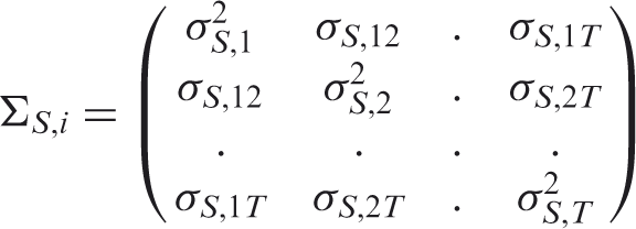
CTT approach is based on a score. It is assumed that a true score exists and that the observed score allows estimating this true score.¹⁶ These two scores are linearly associated.² With the SM method, the patient’s score is computed at each time. The observed score ( $S_{i}^{(t)}$ ) for a patient i ( $i = 1, \dots, N$ ) at one time is obtained by summing his responses ( $y_{ij}^{(t)}$ ) to the J items ( $j = 1, \dots, J$ ) at time t ( $t = 1, \dots, T$ ). A linear mixed model is then fitted on the observed scores in order to test whether a time effect exists.

S_{i} = X_{i} β + e_{S, i} X_{i} β = (μ_{S, i}^{(1)}, μ_{S, i}^{(2)}, \dots, μ_{S, i}^{(T)})' S_{i} ~ N (X_{i} β, Σ_{S, i}) e_{S, i} ~ N (0, Σ_{S, i})

(1)

where

(μ_{S, i}^{(1)}, μ_{S, i}^{(2)}, \dots, μ_{S, i}^{(T)})

represents the vector of the mean scores at times

(1, 2, \dots, T)

and

Σ_{S, i}

is the

(n_{S, i} \times n_{S, i})

covariance matrix of error terms. Since it is possible that the number of answers for each patient is not the same, the parameters depend on the patient (i). For the following analyses, an unstructured covariance matrix will be used assuming that all covariances and variances parameters can be different between times of assessments.

Σ_{S, i} = (σ_{S, 1}^{2} σ_{S, 12} . σ_{S, 1 T} σ_{S, 12} σ_{S, 2}^{2} . σ_{S, 2 T} . . . . σ_{S, 1 T} σ_{S, 2 T} . σ_{S, T}^{2})

Figure 1.

Schematic outline of methods used to simulate and to analyse datasets.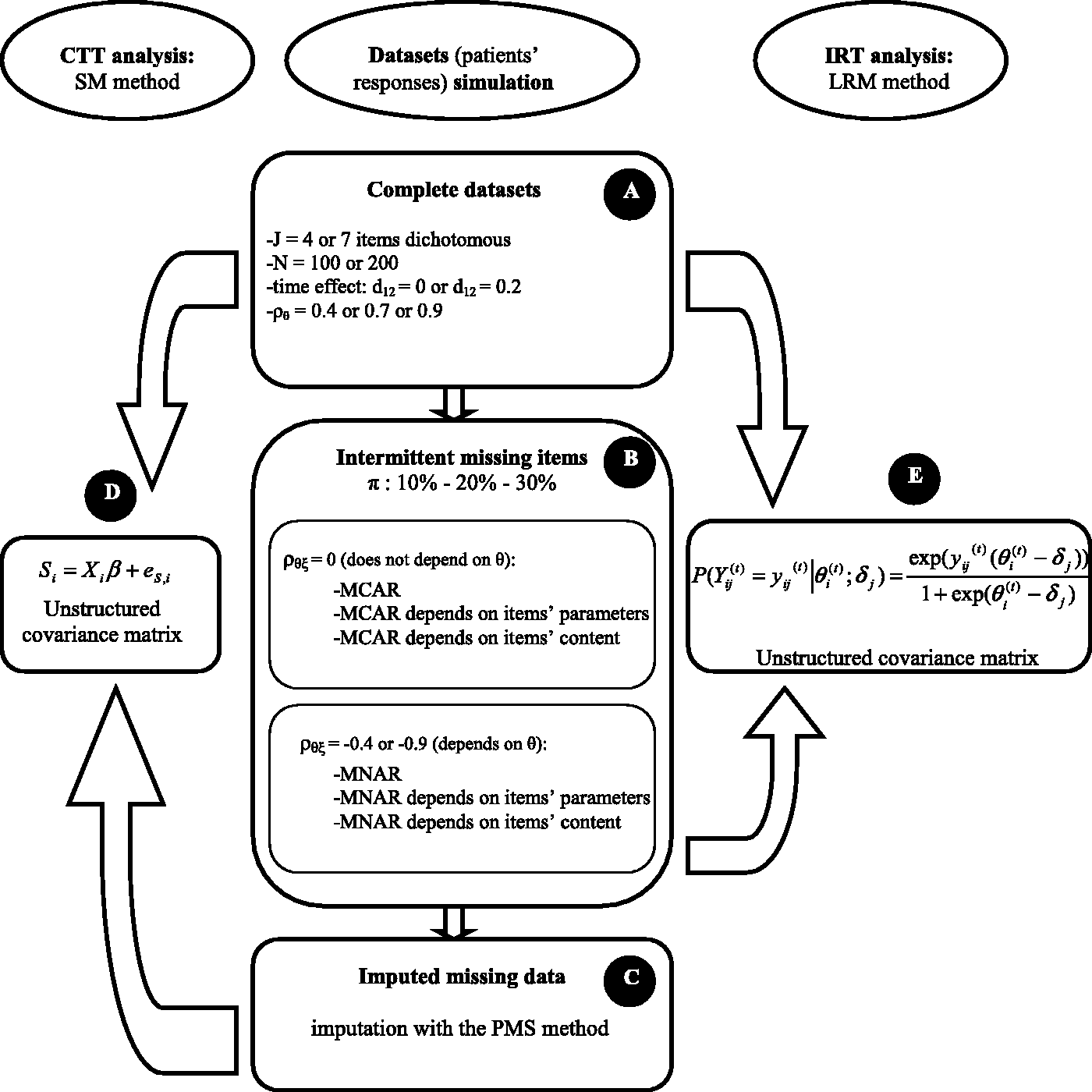

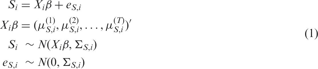
In presence of intermittent missing items, the computation of the score cannot be performed if at least one item is missing. Some scoring manuals of scales (SF-36, QLQ-C30) recommend imputing a missing value by the mean response of the patient to the other items in order to decrease the rate of missing values. This method is named personal mean score (PMS)¹⁷ and is generally used when the amount of missing items at a given time t does not exceed 50% for a given patient (SF-36 manual).¹⁸ Otherwise the score is not computed. The PMS imputation was used before applying SM method.

The restricted maximum likelihood (REML) estimation in SAS Proc MIXED was used to estimate parameters of the model.¹⁹

2.1.2 LRM method (Figure 1, part E)

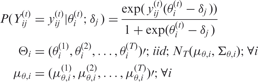
For the Rasch-family models, the probability of a response to an item is modelled as a function of the latent trait and of parameters characterizing the items. The LRM belongs to the Rasch-family models which rely on fundamental assumptions. First, all responses to items must be influenced by the same concept (unidimensionality). Secondly, the probability to obtain a positive answer (the most favourable response regarding the latent trait) to an item increases with the latent trait (monotonicity). Last, the answer to an item for a patient is independent of answers of this patient to other items (local independence). The LRM method is a longitudinal counterpart of the Rasch model.^20–22 The relationship between the items’ answers and the latent variable is modelled by a logistic link function.

P (Y_{ij}^{(t)} = y_{ij}^{(t)} | θ_{i}^{(t)}; δ_{j}) = \frac{\exp (y_{ij}^{(t)} (θ_{i}^{(t)} - δ_{j}))}{1 + \exp (θ_{i}^{(t)} - δ_{j})} Θ_{i} = (θ_{i}^{(1)}, θ_{i}^{(2)}, \dots, θ_{i}^{(T)})'; iid; N_{T} (μ_{θ, i}, Σ_{θ, i}); \forall i μ_{θ, i} = (μ_{θ, i}^{(1)}, μ_{θ, i}^{(2)}, \dots, μ_{θ, i}^{(T)})'; \forall i

(2)

Θ_{i}

corresponds to the patient’s latent trait and has a multivariate normal distribution. The items’ parameters

(Δ_{J} = (δ_{1}, δ_{2}, δ_{3}, \dots, δ_{J})

for J items) are constant over time. An item parameter is a feature of the item, which induces that the amount of positive answers is not the same according to the considered item. Indeed, when the item parameter is higher, the probability of positive answers is lower. The marginal likelihood (MML estimation) was maximized to estimate jointly the items parameters, the mean parameters

μ_{θ}

and the covariance parameters

Σ_{θ}

of the model.

L (Δ_{J}, μ_{θ}, Σ_{θ} | y) = Π_{i = 1}^{N} \int_{ℝ^{T}} Π_{t = 1}^{T} Π_{j = 1}^{J} \frac{\exp (y_{ij}^{(t)} (θ^{(t)} - δ_{j}))}{1 + \exp (θ^{(t)} - δ_{j})} G (θ | μ_{θ, i}, Σ_{θ, i}) d θ

(3)

G (θ | μ_{θ, i}, Σ_{θ, i})

is the multivariate normal distribution function with mean vector

μ_{θ, i}

and an unstructured covariance matrix

Σ_{θ, i}

Σ_{θ, i} = (σ_{θ, 1}^{2} σ_{θ, 12} . σ_{θ, 1 T} σ_{θ, 12} σ_{θ, 2}^{2} . σ_{θ, 2 T} . . . . σ_{θ, 1 T} σ_{θ, 2 T} . σ_{θ, T}^{2})

Gllamm in Stata has been used to estimate parameters of the model.²³

2.2 Longitudinal PROs simulation

As our purpose was to evaluate the performance of both methods, a simulation study was used. Datasets that follow a given statistical model and several defined assumptions can be created using simulation. In that case, the parameters’ values used to simulate datasets can be considered as their true values. Thus, by analysing these datasets, estimated parameters can be compared to the true values and possible bias are deduced.²⁴ The bias of the time effect estimations, the type I error and the power of the tests were examined. A t-test was used in order to compare the means of the time effect estimation (means obtained with SM and LRM methods) to the true value (simulated value) and, therefore to conclude about the potential bias of this estimation. The number of time effect estimations that were above, below or equal to the time effect true value was computed and a sign test was used for comparing SM and LRM methods. The type I error was determined as the proportion of rejection of the null hypothesis H₀ (H₀: there is no time effect) for all of the simulated datasets corresponding to each case where no time effect had been simulated. The power was computed as the rate of rejection of H₀ for all of the simulated datasets corresponding to each case where a time effect had been simulated. The expected rate for the type I error was 5%.

2.2.1 Complete datasets (Figure 1, part A)

In a first step, complete datasets which represented PROs data were simulated. We assumed that the corresponding PROs had been previously validated with both score and Rasch-based approaches as it is currently performed nowadays.^25–27 This corresponds to the situation where PROs are intended to be analysed using either a Rasch-based model or a CTT approach. Indeed, the assumptions required for the analysis of data with a CTT approach are necessarily fulfilled when data satisfy the assumptions of a Rasch model.²⁸ The design of the simulated study involved dichotomous items with three times of assessment for scales containing four or seven items. The patients’ responses were simulated using Monte Carlo simulations with a longitudinal Rasch model.¹⁴

The time effect between two consecutive measures was $d_{t, t + 1} = μ_{θ}^{(t + 1)} - μ_{θ}^{(t)}$ . Two assumptions regarding time effect were simulated: time effect or no time effect. When no time effect was simulated: $d_{12} = μ_{θ}^{(2)} - μ_{θ}^{(1)} = 0 = d_{23}$ . When a time effect was simulated: $d_{12} = μ_{θ}^{(2)} - μ_{θ}^{(1)} = 0.2 = d_{23}$ . When no time effect was simulated ( $d_{12} = 0 = d_{23}$ ), the true time effect was known for both methods (0). However, when a time effect was simulated ( $d_{12} = 0.2 = d_{23}$ ) the true time effect was only known for LRM because simulations were based on the Rasch model but it was not for SM. Indeed, datasets were simulated using the latent trait but not the score. One can estimate the true time effect for SM using Gauss-Hermite quadratures based on the difference of the computed expected score between two consecutive times as explained in Ref. 15. Thus, for SM, d₁₂ _SM and d₂₃ _SM were equal to 0, when no time effect was simulated. When a time effect was simulated, d₁₂ _SM and d₂₃ _SM were equal to 0.15 and to 0.25 for respectively the four-item scale and the seven-item scale.

The items’ parameters were regularly distributed and defined by the vectors Δ₄ and Δ₇ for respectively the four-items scale and the seven-items scale.

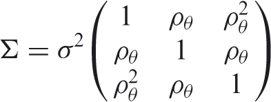
The latent trait vector $Θ = (θ^{(1)}, θ^{(2)}, θ^{(3)})'$ followed a multivariate normal distribution with mean $μ_{θ} = (μ_{θ}^{(1)}, μ_{θ}^{(2)}, μ_{θ}^{(3)})'$ and with a first-order autoregressive structure of covariance matrix Σ.

Σ = σ^{2} (1 ρ_{θ} ρ_{θ}^{2} ρ_{θ} 1 ρ_{θ} ρ_{θ}^{2} ρ_{θ} 1)

This structure assumed that correlations between two consecutive measures decrease exponentially with the distance between two consecutive times. Three different values for the correlation coefficient of the latent trait between two consecutive times ( $ρ_{θ}$ ) were used to simulate data: 0.4 or 0.7 or 0.9.

Five-hundred datasets were simulated for each case.

2.2.2 Intermittent missing items (Figure 1, part B)

In a second step, different types of intermittent missing items (informative or non-informative) were generated from the complete simulated datasets.

The intermittent missing items were simulated using a variable (ξ), which represented the non-response propensity. ( $ξ_{i}^{(1)}, ξ_{i}^{(2)}, ξ_{i}^{(3)}$ ) followed a standardized multinormal distribution. The correlation coefficient $ρ_{θ ξ}$ between the latent variable of interest θ and the patient’s propensity of non-response ξ was simulated equal to 0 for MCAR items (non-informative missing items because θ and ξ were independent) and equal to −0.4 or −0.9 for MNAR items. Indeed, we assumed that patients with poorer quality of life were less likely to respond to items. Correlations were thus assumed to be negative and used as such to simulate informative intermittent missing items. The intermittent missing items process was simulated using the following model:^13,29

P (D_{ij}^{(t)} = 1 | ξ_{i}^{(t)}, δ_{j}, π_{\min}^{(j)}, π_{\max}^{(j)}) = π_{\min}^{(j)} + (π_{\max}^{(j)} - π_{\min}^{(j)}) \frac{\exp (ξ_{i}^{(t)} + w δ_{j})}{1 + \exp (ξ_{i}^{(t)} + w δ_{j})}

(4)

where

D_{ij}^{(t)} = 1

represents the situation where the jth item is missing at time t for a patient i and

D_{ij}^{(t)} = 0

otherwise. Different rates of intermittent missing items were simulated:

π = 10 %

or 20% or 30%.

π_{\min}^{(j)}

is the minimum individual probability of non-response for an item j at time t (for a very low value of ξ) and

π_{\max}^{(j)}

is its maximum (for a very large value of ξ).

π_{\min}^{(j)}

was fixed at 1% and

π_{\max}^{(j)}

was fixed at

2 π - 1 %

with the average rate of intermittent missing items π equal to

(π_{\min}^{(j)} + π_{\max}^{(j)}) / 2

. In our simulation study, missing items mechanism can depend on the items’ parameters (

δ_{j}

) (when w = 1) or not (when w = 0). If w = 1, we considered that as the item’s parameter value got higher, the probability of missing answers to this item increased. The item content can impact the missing items mechanism as well. For instance, contents dealing with very personal topics (sexual, spiritual…) may engender high rate of missing answers to this item. For the first item on the four-item scale and for the second one on the seven-item scale, a potentially personal content was simulated by increasing

π_{\min}^{(j)}

and

π_{\max}^{(j)}

2 π

The PMS imputation has only been used when the amount of missing items did not exceed 50% for a given patient. Thus, one and three items maximum were imputed for the four-item scale and the seven-item scale, respectively.

3 Results

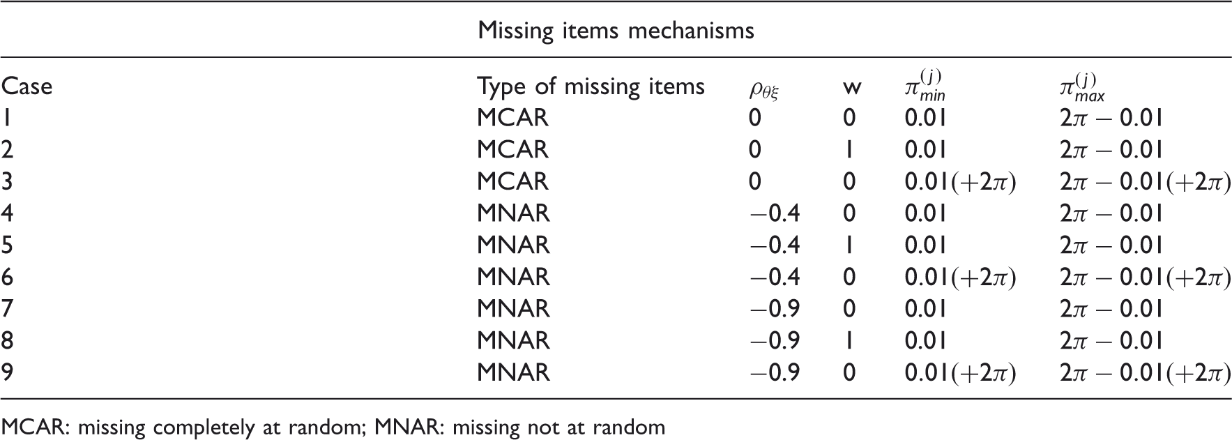
Tables 2 to 5 give the results (bias when no time effect was simulated, type I error, bias when a time effect was simulated and power) for datasets obtained with the mechanisms numbered 1, 4 and 7 (MCAR and MNAR cases) detailed in Table 1. The items’ parameters and the content of items are not involved in the missing data mechanisms for these datasets (w = 0).

Table 1.

Parameters used for complete datasets simulation and missing items mechanisms with N the sample size, T the number of assessments, J the number of items, Δ _J the vector of items’ parameters, $μ_{θ}$ the vector of the times measurement, $ρ_{θ}$ the correlation coefficient of the latent trait between two consecutive times, $σ^{2}$ the variance of the latent trait, $ρ_{θ ξ}$ the correlation between the latent variable of interest and the patient’s propensity of non-response, w the link between the items’ parameters and the patient’s propensity of non-response, $π_{\min}^{(j)}$ the minimum individual probability of non-response for an item j at time t for a very low value of ξ and $π_{\max}^{(j)}$ the maximum one for a very large value of ξ.

Complete datasets simulation
Parameters	Simulated values
$μ_{θ}$	No time effect (0, 0, 0) or Time effect (−0.2, 0, 0.2)
N	100 or 200
T	3
J	4 or 7
$Δ_{J}$	$Δ_{4} = (- 1, - 0.5, 0.5, 1)$ or $Δ_{7} = (- 1.5, - 1, - 0.5, 0, 0.5, 1, 1.5)$
$ρ_{θ}$	0.4 or 0.7 or 0.9
$σ^{2}$	1
Number of datasets for each simulated case	500
Missing items mechanisms
Case	Type of missing items	$ρ_{θ ξ}$	w	$π_{\min}^{(j)}$	$π_{\max}^{(j)}$
1	MCAR	0	0	0.01	$2 π - 0.01$
2	MCAR	0	1	0.01	$2 π - 0.01$
3	MCAR	0	0	$0.01 (+ 2 π)$	$2 π - 0.01 (+ 2 π)$
4	MNAR	−0.4	0	0.01	$2 π - 0.01$
5	MNAR	−0.4	1	0.01	$2 π - 0.01$
6	MNAR	−0.4	0	$0.01 (+ 2 π)$	$2 π - 0.01 (+ 2 π)$
7	MNAR	−0.9	0	0.01	$2 π - 0.01$
8	MNAR	−0.9	1	0.01	$2 π - 0.01$
9	MNAR	−0.9	0	$0.01 (+ 2 π)$	$2 π - 0.01 (+ 2 π)$

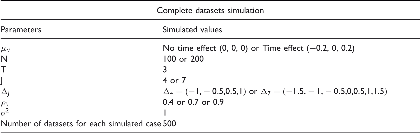
MCAR: missing completely at random; MNAR: missing not at random

Table 2.

Time effect estimation between time 2 and time 1 ( ${\overset{\land}{d}}_{12}$ ) and standard deviations (s.d.) when no time effect was simulated for score mixed model (SM) with personal mean score (PMS) imputation or without and longitudinal Rasch mixed model (LRM) methods for different values of sample size (N), number of items (J), latent variable correlation ( $ρ_{θ}$ ), proportion of missing data (π) and for three cases (complete case, MCAR with $ρ_{θ ξ} = 0$ , MNAR with $ρ_{θ ξ} = - 0.4$ or −0.9). Analyses performed with an unstructured covariance matrix in SM and LRM methods.

N	J	$ρ_{θ}$	π (%)	$d_{12 LRM}$ $= d_{12 SM} §$	Complete data				MCAR				MNAR
					$ρ_{θ ξ} = 0$				$ρ_{θ ξ} = - 0.4$				$ρ_{θ ξ} = - 0.9$
					LRM		SM		LRM		SM		LRM		SM		LRM		SM
					${\overset{\land}{d}}_{12}$	s.d.	${\overset{\land}{d}}_{12}$	s.d.	${\overset{\land}{d}}_{12}$	s.d.	${\overset{\land}{d}}_{12}$	s.d.	${\overset{\land}{d}}_{12}$	s.d.	${\overset{\land}{d}}_{12}$	s.d.	${\overset{\land}{d}}_{12}$	s.d.	${\overset{\land}{d}}_{12}$	s.d.
100	4	0.4	0	0	−0.017	0.210	−0.012	0.158
10	0.020	0.212	0.015	0.162	−0.001	0.213	0.001	0.164	0.007	0.212	0.009	0.165
20	−0.023	0.228	−0.011	0.187	0.015	0.209	0.005	0.171	0.019	0.227	0.007	0.184
30	0.004	0.235	0.004	0.205	−0.002	0.233	−0.001	0.208	−0.008	0.231	−0.007	0.200
0.7	0	0.003	0.185	0.002	0.138
10	−0.014	0.182	−0.010	0.139	0.009	0.194	0.008	0.153	−0.003	0.198	−0.002	0.149
20	0.012	0.206	0.008	0.167	0.004	0.209	0.003	0.163	−0.015	0.215	−0.017	0.174
30	0.014	0.229	0.013	0.198	−0.006	0.222	−0.009	0.199	−0.014	0.216	−0.015	0.194
0.9	0	−0.014	0.168	−0.009	0.123
10	0.002	0.177	0.002	0.134	0.014	0.191	0.010	0.141	−0.004	0.189	−0.006	0.146
20	−0.009	0.194	−0.002	0.158	0.003	0.199	−0.003	0.161	−0.007	0.189	−0.007	0.151
30	0.014	0.211	0.014	0.182	−0.004	0.208	−0.009	0.182	−0.009	0.210	−0.011	0.185
7	0.4	0	0	−0.006	0.171	−0.007	0.212
10	0.004	0.170	0.006	0.216	0.009	0.181	0.014	0.231	0.002	0.172	0.004	0.218
20	−0.008	0.185	−0.009	0.239	−0.002	0.181	0.001	0.230	0.017	0.195	0.019	0.251
30	−0.013	0.190	−0.022	0.258	−0.017	0.194	−0.018	0.257	0.007	0.182	0.001	0.253
0.7	0	0.009	0.148	0.011	0.185
10	−0.002	0.157	−0.002	0.199	−0.001	0.153	−0.002	0.196	−0.013	0.156	−0.012	0.200
20	0.014	0.163	0.019	0.211	0.000	0.163	−0.002	0.210	−0.009	0.162	−0.011	0.216
30	0.007	0.178	0.018	0.240	0.007	0.185	0.000	0.260	0.004	0.177	0.010	0.241
0.9	0	−0.005	0.133	−0.007	0.165
10	0.004	0.144	0.004	0.186	−0.005	0.144	−0.004	0.184	−0.011	0.141	−0.009	0.177
20	−0.010	0.150	−0.015	0.196	0.001	0.155	0.008	0.204	−0.010	0.146	−0.008	0.188
30	−0.004	0.161	−0.010	0.227	−0.010	0.176	−0.016	0.239	0.007	0.172	0.009	0.238
200	4	0.4	0	0	0.004	0.148	0.003	0.111
10	0.009	0.137	0.008	0.107	−0.007	0.150	−0.005	0.117	0.003	0.146	0.000	0.112
20	0.002	0.164	0.001	0.133	0.001	0.146	0.002	0.121	−0.002	0.160	−0.002	0.127
30	−0.008	0.165	−0.006	0.145	−0.012	0.158	−0.014	0.148	−0.002	0.172	−0.008	0.148
0.7	0	−0.006	0.131	−0.005	0.098
10	−0.012	0.132	−0.009	0.104	0.011	0.139	0.008	0.107	0.004	0.125	0.001	0.098
20	−0.009	0.148	−0.004	0.120	−0.015	0.144	−0.012	0.118	0.003	0.142	−0.003	0.122
30	0.006	0.148	0.002	0.132	−0.006	0.148	−0.002	0.131	−0.010	0.148	−0.009	0.133
0.9	0	0.002	0.118	0.001	0.088
10	0.000	0.127	−0.001	0.099	0.004	0.130	0.004	0.102	0.006	0.128	0.005	0.100
20	0.000	0.132	−0.004	0.106	−0.001	0.137	−0.002	0.115	−0.008	0.137	−0.006	0.112
30	0.001	0.141	0.003	0.128	−0.011	0.150	−0.006	0.136	−0.006	0.145	−0.013	0.123
7	0.4	0	0	−0.008	0.119	−0.011	0.149
10	−0.003	0.122	−0.005	0.156	0.005	0.125	0.007	0.158	−0.002	0.119	−0.002	0.150
20	−0.005	0.133	−0.010	0.170	−0.001	0.123	−0.001	0.160	−0.005	0.127	−0.009	0.166
30	0.003	0.135	0.004	0.189	−0.004	0.136	−0.012	0.189	0.003	0.150	−0.002	0.207
0.7	0	0.007	0.102	0.009	0.128
10	−0.006	0.107	−0.007	0.137	0.001	0.110	0.003	0.140	−0.004	0.111	−0.003	0.140
20	0.008	0.113	0.008	0.152	0.002	0.117	0.004	0.154	−0.007	0.114	−0.007	0.149
30	0.001	0.125	0.001	0.174	−0.003	0.115	−0.011	0.157	−0.007	0.124	−0.016	0.170
0.9	0	0.002	0.096	0.002	0.120
10	0.003	0.105	0.005	0.133	−0.004	0.102	−0.004	0.130	−0.005	0.102	−0.005	0.131
20	0.001	0.106	−0.001	0.137	−0.002	0.108	0.002	0.141	−0.003	0.104	−0.008	0.139
30	0.006	0.118	0.012	0.163	−0.005	0.105	−0.010	0.152	−0.006	0.106	−0.014	0.148

Tables 2 to 5 show the results for complete datasets and for intermittent missing items (the items’ parameters and the content of items do not play a role in missing data mechanisms for these datasets).

MCAR: missing completely at random; MNAR: missing not at random

Italicised numbers indicate that the t−test comparing the time effect estimation ${\overset{\land}{d}}_{12}$ and the time effect true value d₁₂ is significant at 5%. It shows that the time effect estimation is biased at the 5% level.

§: according to Blanchin et al.¹⁵

Table 3.

Type I error of the tests of time effect for score mixed model (SM) with personal mean score (PMS) imputation or without and longitudinal Rasch mixed model (LRM) methods for different values of sample size (N), number of items (J), latent variable correlation ( $ρ_{θ}$ ), proportion of missing data (π) and for three cases (complete case, MCAR with $ρ_{θ ξ} = 0$ , MNAR with $ρ_{θ ξ} = - 0.4$ or −0.9). Analyses performed with an unstructured covariance matrix in SM and LRM methods.

N	J	$ρ_{θ}$	π (%)	Complete data		MCAR		MNAR
				LRM	SM	$ρ_{θ ξ} = 0$		$ρ_{θ ξ} = - 0.4$		$ρ_{θ ξ} = - 0.9$
				LRM	SM	LRM	SM	LRM	SM	LRM	SM
100	4	0.4	0	0.060	0.066
10	0.074 *	0.080 *	0.058	0.062	0.066	0.066
20	0.064	0.074	0.040	0.040	0.060	0.074
30	0.044	0.050	0.052	0.058	0.042	0.074
0.7	0	0.044	0.046
10	0.038	0.046	0.058	0.080*	0.048	0.056
20	0.046	0.066	0.040	0.032*	0.054	0.050
30	0.052	0.072	0.064	0.090*	0.048	0.070
0.9	0	0.050	0.054
10	0.034	0.046	0.070	0.082*	0.060	0.076*
20	0.046	0.062	0.036	0.044	0.034	0.042
30	0.054	0.060	0.036	0.052	0.044	0.064
7	0.4	0	0.068	0.070
10	0.062	0.066	0.060	0.054	0.054	0.058
20	0.060	0.060	0.054	0.058	0.058	0.058
30	0.058	0.056	0.054	0.046	0.038	0.052
0.7	0	0.062	0.064
10	0.066	0.066	0.072	0.084*	0.050	0.048
20	0.046	0.062	0.066	0.074	0.046	0.066
30	0.054	0.044	0.078*	0.084*	0.054	0.054
0.9	0	0.052	0.054
10	0.062	0.068	0.054	0.062	0.056	0.062
20	0.052	0.056	0.052	0.054	0.051	0.054
30	0.046	0.068	0.062	0.068	0.067	0.088*
200	4	0.4	0	0.074*	0.072
10	0.040	0.038	0.064	0.070	0.050	0.056
20	0.066	0.060	0.040	0.054	0.056	0.054
30	0.062	0.068	0.060	0.060	0.050	0.070
0.7	0	0.074*	0.072
10	0.046	0.052	0.062	0.054	0.048	0.038
20	0.060	0.064	0.062	0.056	0.042	0.048
30	0.038	0.042	0.036	0.036	0.060	0.052
0.9	0	0.034	0.030*
10	0.046	0.054	0.038	0.050	0.050	0.052
20	0.038	0.044	0.054	0.058	0.046	0.056
30	0.042	0.036	0.060	0.066	0.056	0.042
7	0.4	0	0.042	0.042
10	0.044	0.052	0.046	0.052	0.054	0.054
20	0.032*	0.036	0.046	0.052	0.050	0.056
30	0.050	0.046	0.058	0.068	0.066	0.072
0.7	0	0.036	0.038
10	0.048	0.048	0.038	0.042	0.058	0.058
20	0.048	0.052	0.056	0.058	0.052	0.060
30	0.058	0.056	0.040	0.052	0.042	0.054
0.9	0	0.056	0.058
10	0.066	0.062	0.049	0.050	0.050	0.050
20	0.054	0.060	0.047	0.056	0.036	0.050
30	0.063	0.064	0.043	0.046	0.046	0.068

MCAR: missing completely at random; MNAR: missing not at random

The expected value of 5% is not included in the 95% confidence interval.

Italicised numbers indicate that the time effect estimation ${\overset{\land}{d}}_{12}$ linked to this type I error is biased at the 5% level.

Table 4.

Time effect estimation between time 2 and time 1 ( ${\overset{\land}{d}}_{12}$ ) and standard deviations (s.d.) when a time effect was simulated for score mixed model (SM) with personal mean score (PMS) imputation or without and longitudinal Rasch mixed model (LRM) methods for different values of sample size (N), number of items (J), latent variable correlation ( $ρ_{θ}$ ), proportion of missing data (π) and for three cases (complete case, MCAR with $ρ_{θ ξ} = 0$ , MNAR with $ρ_{θ ξ} = - 0.4$ or −0.9). Analyses performed with an unstructured covariance matrix in SM and LRM methods.

N	J	$ρ_{θ}$	π (%)	$d_{12 LRM}$	$d_{12 SM} §$	Complete data				MCAR				MNAR
						LRM		SM		$ρ_{θ ξ} = 0$				$ρ_{θ ξ} = - 0.4$				$ρ_{θ ξ} = - 0.9$
						LRM		SM		LRM		SM		LRM		SM		LRM		SM
						${\overset{\land}{d}}_{12}$	s.d.	${\overset{\land}{d}}_{12}$	s.d.	${\overset{\land}{d}}_{12}$	s.d.	${\overset{\land}{d}}_{12}$	s.d.	${\overset{\land}{d}}_{12}$	s.d.	${\overset{\land}{d}}_{12}$	s.d.	${\overset{\land}{d}}_{12}$	s.d.	${\overset{\land}{d}}_{12}$	s.d.
100	4	0.4	0	0.2	0.15	0.214	0.196	0.160	0.146
10	0.200	0.193	0.148	0.148	0.200	0.203	0.147	0.154	0.206	0.200	0.153	0.153
20	0.216	0.212	0.162	0.173	0.188	0.221	0.134	0.184	0.207	0.224	0.153	0.180
30	0.207	0.227	0.161	0.206	0.205	0.246	0.151	0.216	0.210	0.227	0.145	0.197
0.7	0	0.200	0.186	0.149	0.137
10	0.205	0.205	0.154	0.157	0.203	0.199	0.147	0.151	0.202	0.195	0.148	0.151
20	0.200	0.209	0.150	0.171	0.200	0.207	0.141	0.169	0.187	0.207	0.136	0.171
30	0.220	0.237	0.170	0.212	0.200	0.202	0.150	0.183	0.214	0.221	0.151	0.203
0.9	0	0.202	0.172	0.151	0.126
10	0.207	0.188	0.155	0.143	0.208	0.179	0.152	0.137	0.203	0.191	0.150	0.144
20	0.200	0.194	0.148	0.159	0.211	0.185	0.160	0.140	0.220	0.198	0.161	0.162
30	0.208	0.215	0.151	0.178	0.201	0.207	0.150	0.185	0.205	0.208	0.152	0.183
7	0.4	0	0.2	0.25	0.201	0.170	0.253	0.213
10	0.186	0.175	0.232	0.221	0.198	0.171	0.249	0.217	0.197	0.174	0.249	0.220
20	0.199	0.188	0.247	0.247	0.215	0.175	0.265	0.230	0.199	0.183	0.245	0.236
30	0.201	0.197	0.245	0.271	0.194	0.192	0.243	0.266	0.203	0.196	0.253	0.261
0.7	0	0.217	0.143	0.272	0.179
10	0.202	0.155	0.253	0.195	0.198	0.165	0.252	0.208	0.203	0.164	0.253	0.204
20	0.218	0.158	0.270	0.205	0.192	0.171	0.241	0.222	0.187	0.168	0.234	0.222
30	0.198	0.188	0.255	0.258	0.208	0.169	0.264	0.237	0.199	0.167	0.252	0.233
0.9	0	0.193	0.141	0.241	0.176
10	0.190	0.149	0.235	0.184	0.210	0.148	0.260	0.186	0.192	0.143	0.241	0.181
20	0.196	0.157	0.241	0.206	0.194	0.157	0.244	0.203	0.193	0.152	0.241	0.198
30	0.195	0.165	0.250	0.226	0.201	0.161	0.257	0.225	0.198	0.167	0.243	0.237
200	4	0.4	0	0.2	0.15	0.206	0.143	0.155	0.107
10	0.196	0.149	0.147	0.115	0.198	0.145	0.149	0.113	0.195	0.142	0.146	0.107
20	0.208	0.157	0.156	0.125	0.199	0.154	0.154	0.126	0.205	0.168	0.155	0.135
30	0.194	0.170	0.148	0.150	0.191	0.159	0.147	0.137	0.200	0.166	0.147	0.147
0.7	0	0.203	0.127	0.152	0.095
10	0.195	0.138	0.143	0.107	0.210	0.131	0.160	0.102	0.197	0.147	0.147	0.111
20	0.199	0.142	0.146	0.116	0.202	0.146	0.152	0.118	0.198	0.146	0.149	0.118
30	0.208	0.159	0.153	0.141	0.192	0.154	0.142	0.138	0.183	0.156	0.142	0.134
0.9	0	0.204	0.127	0.152	0.094
10	0.203	0.135	0.149	0.100	0.218	0.139	0.160	0.106	0.208	0.137	0.155	0.106
20	0.202	0.138	0.149	0.110	0.196	0.144	0.144	0.115	0.197	0.131	0.148	0.106
30	0.206	0.153	0.155	0.129	0.198	0.148	0.147	0.130	0.200	0.142	0.149	0.134
7	0.4	0	0.2	0.25	0.207	0.114	0.259	0.143
10	0.209	0.123	0.261	0.156	0.188	0.132	0.235	0.168	0.196	0.124	0.245	0.158
20	0.205	0.124	0.255	0.162	0.197	0.132	0.245	0.167	0.204	0.127	0.257	0.166
30	0.208	0.135	0.265	0.183	0.204	0.133	0.256	0.184	0.181	0.141	0.230	0.199
0.7	0	0.200	0.106	0.251	0.133
10	0.195	0.110	0.243	0.138	0.197	0.116	0.251	0.146	0.201	0.109	0.252	0.139
20	0.199	0.115	0.249	0.149	0.201	0.117	0.253	0.154	0.191	0.119	0.234	0.156
30	0.203	0.123	0.256	0.169	0.187	0.118	0.229	0.173	0.197	0.125	0.242	0.172
0.9	0	0.201	0.092	0.251	0.115
10	0.209	0.098	0.260	0.123	0.206	0.101	0.258	0.130	0.198	0.101	0.249	0.127
20	0.199	0.105	0.246	0.140	0.196	0.104	0.246	0.139	0.194	0.107	0.243	0.139
30	0.205	0.116	0.258	0.163	0.198	0.109	0.249	0.153	0.197	0.110	0.242	0.154

MCAR: missing completely at random; MNAR: missing not at random

Italicised numbers indicate that the t-test comparing the time effect estimation ${\overset{\land}{d}}_{12}$ and the time effect true value d₁₂ is significant at 5%. It shows that the time effect estimation is biased at the 5% level.

§: according to Blanchin et al.¹⁵

Table 5.

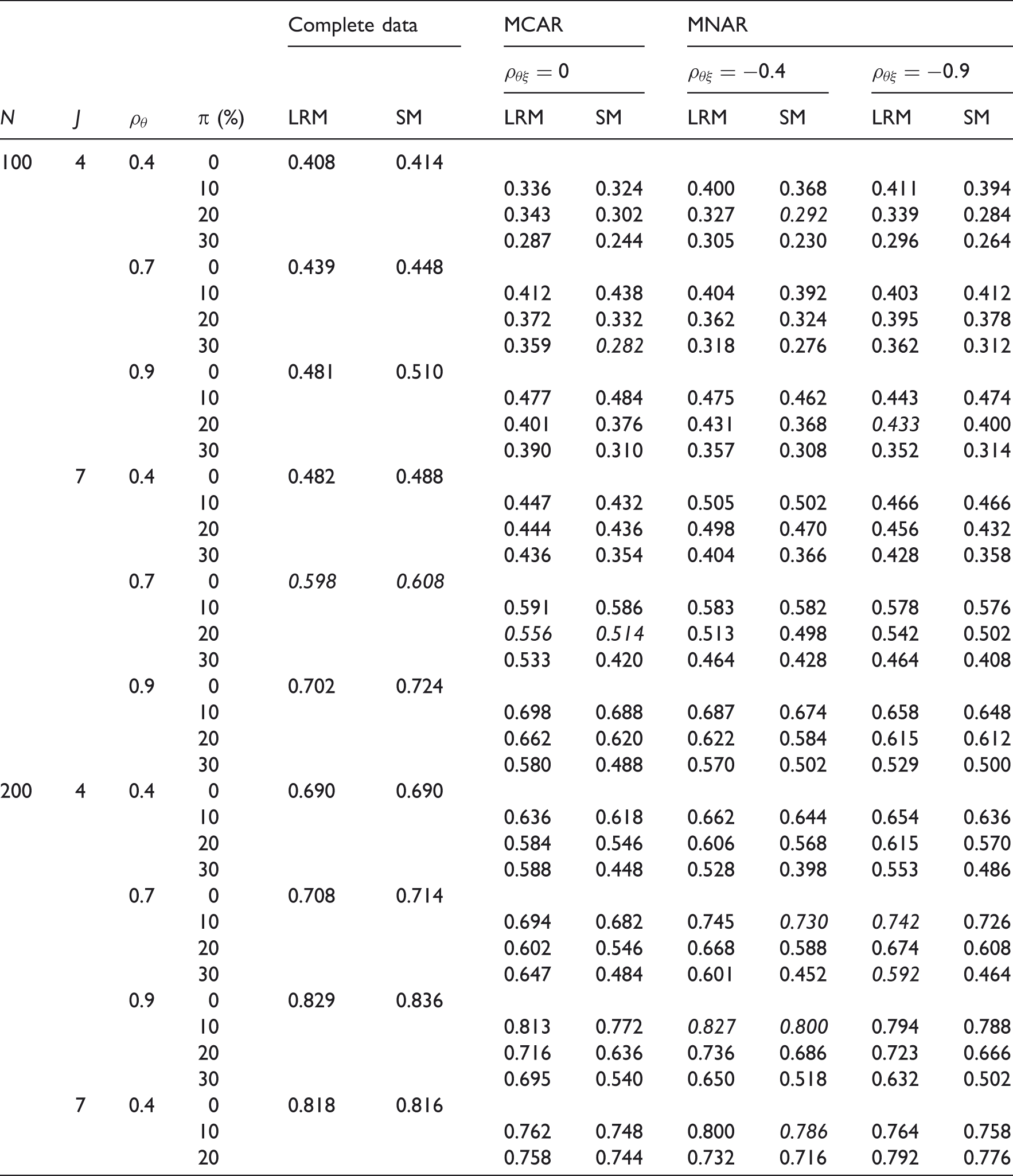
Power of the tests of time effect for score mixed model (SM) with personal mean score (PMS) imputation or without and longitudinal Rasch mixed model (LRM) methods for different values of sample size (N), number of items (J), latent variable correlation ( $ρ_{θ}$ ), proportion of missing data (π) and for three cases (complete case, MCAR with $ρ_{θ ξ} = 0$ , MNAR with $ρ_{θ ξ} = - 0.4$ or −0.9). Analyses performed with an unstructured covariance matrix in SM and LRM methods.

N	J	$ρ_{θ}$	π (%)	Complete data		MCAR		MNAR
				$ρ_{θ ξ} = 0$		$ρ_{θ ξ} = - 0.4$		$ρ_{θ ξ} = - 0.9$
				LRM	SM	LRM	SM	LRM	SM	LRM	SM
100	4	0.4	0	0.408	0.414
10	0.336	0.324	0.400	0.368	0.411	0.394
20	0.343	0.302	0.327	0.292	0.339	0.284
30	0.287	0.244	0.305	0.230	0.296	0.264
0.7	0	0.439	0.448
10	0.412	0.438	0.404	0.392	0.403	0.412
20	0.372	0.332	0.362	0.324	0.395	0.378
30	0.359	0.282	0.318	0.276	0.362	0.312
0.9	0	0.481	0.510
10	0.477	0.484	0.475	0.462	0.443	0.474
20	0.401	0.376	0.431	0.368	0.433	0.400
30	0.390	0.310	0.357	0.308	0.352	0.314
7	0.4	0	0.482	0.488
10	0.447	0.432	0.505	0.502	0.466	0.466
20	0.444	0.436	0.498	0.470	0.456	0.432
30	0.436	0.354	0.404	0.366	0.428	0.358
0.7	0	0.598	0.608
10	0.591	0.586	0.583	0.582	0.578	0.576
20	0.556	0.514	0.513	0.498	0.542	0.502
30	0.533	0.420	0.464	0.428	0.464	0.408
0.9	0	0.702	0.724
10	0.698	0.688	0.687	0.674	0.658	0.648
20	0.662	0.620	0.622	0.584	0.615	0.612
30	0.580	0.488	0.570	0.502	0.529	0.500
200	4	0.4	0	0.690	0.690
10	0.636	0.618	0.662	0.644	0.654	0.636
20	0.584	0.546	0.606	0.568	0.615	0.570
30	0.588	0.448	0.528	0.398	0.553	0.486
0.7	0	0.708	0.714
10	0.694	0.682	0.745	0.730	0.742	0.726
20	0.602	0.546	0.668	0.588	0.674	0.608
30	0.647	0.484	0.601	0.452	0.592	0.464
0.9	0	0.829	0.836
10	0.813	0.772	0.827	0.800	0.794	0.788
20	0.716	0.636	0.736	0.686	0.723	0.666
30	0.695	0.540	0.650	0.518	0.632	0.502
7	0.4	0	0.818	0.816
10	0.762	0.748	0.800	0.786	0.764	0.758
20	0.758	0.744	0.732	0.716	0.792	0.776
30	0.724	0.650	0.730	0.678	0.706	0.644
0.7	0	0.908	0.908
10	0.860	0.850	0.868	0.864	0.861	0.856
20	0.846	0.802	0.825	0.794	0.816	0.804
30	0.775	0.700	0.753	0.664	0.816	0.712
0.9	0	0.956	0.954
10	0.937	0.928	0.949	0.946	0.927	0.918
20	0.914	0.886	0.919	0.890	0.903	0.888
30	0.876	0.796	0.889	0.814	0.877	0.780

MCAR: missing completely at random; MNAR: missing not at random

Italicised numbers indicate that the time effect estimation ${\overset{\land}{d}}_{12}$ linked to this power is biased at the 5% level.

3.1 Complete datasets

For complete datasets, similar results were observed for SM and LRM methods regarding type I error and power. The type I errors were close to the expected value (5%). Both methods displayed unbiased results and similar power whatever the values of the parameters (results ‘complete data’ in all tables).

3.2 Intermittent missing items (item non-response)

Table 2 shows the results of the time effect estimation between time 2 and time 1 when no time effect was simulated. Globally, there were more biased values for SM as compared to LRM method (eight for SM and four for LRM). Biased values concerned more often MNAR data than MCAR data (respectively eight- and four-biased values) with six MNAR-biased values for SM and only two for LRM. These results were comparable to those corresponding to the time effect estimation between time 3 and time 2 (results not shown). The number of times means of the time effect estimations between time 2 and time 1 were above, below or equal to the true value of the time effect seemed to be similar for both methods (two significant sign tests for SM and one for LRM).

Table 3 shows results of the type I error. The type I errors were close to the expected value (minimum: 3%, mean: 5% and maximum: 9%). The number of patients and items, the correlation of the latent trait between two consecutive times, the correlation between the latent trait θ and the variable ξ seemed to have no influence on the type I error. Results were similar whatever the type (MCAR or MNAR) or rate (10%, 20% and 30%) of missing items. Therefore, it seemed that the type I error was controlled for SM and LRM.

Table 4 shows results of the time effect estimation between time 2 and time 1 when a time effect was simulated. Quite similarly as the case where no time effect was simulated, SM engendered slightly more biased values than LRM: seven for SM and five for LRM. Moreover, MNAR data were more often impacted than MCAR data by these biases. These results were comparable to those corresponding to the time effect estimation between time 3 and time 2 (results not shown). The number of times means of the time effect estimations between time 2 and time 1 were above, below or equal to the true value of the time effect seemed to be similar for both methods (only one significant sign test for SM).

Table 5 presents results on the power of time effect tests. Some power must be interpreted with caution because the associated time effect estimations were biased. Several parameters impacted power for both methods and for all types of intermittent missing items (MCAR or MNAR): the number of patients and of items and the correlation between two consecutive times. As expected, when the sample size was lower, the power decreased, and it increased with the number of items. Similarly, when the correlation of the latent trait between two consecutive times was higher, the observed power increased.

By contrast with the type I error which was not impacted, power decreased when the rate of intermittent missing items increased. However, it could be noticed that the loss of power induced by an increase of the rate of intermittent missing items was lower for LRM than for SM. No variation could really be explained by the type of intermittent missing items for SM and for LRM and conclusions were indeed the same for MCAR and MNAR items.

For the LRM method, power was overall higher than the one obtained with SM method, whatever the values of the parameters and the type of intermittent missing items (Figure 2). The difference in power between LRM and SM ranged from 0.01 to 0.20.

Figure 2.

Comparison of power of the tests of time effect for score mixed model (SM) with PMS imputation and longitudinal Rasch mixed model (LRM) methods for one case: sample size (N = 200), number of items (J = 7), latent variable correlation (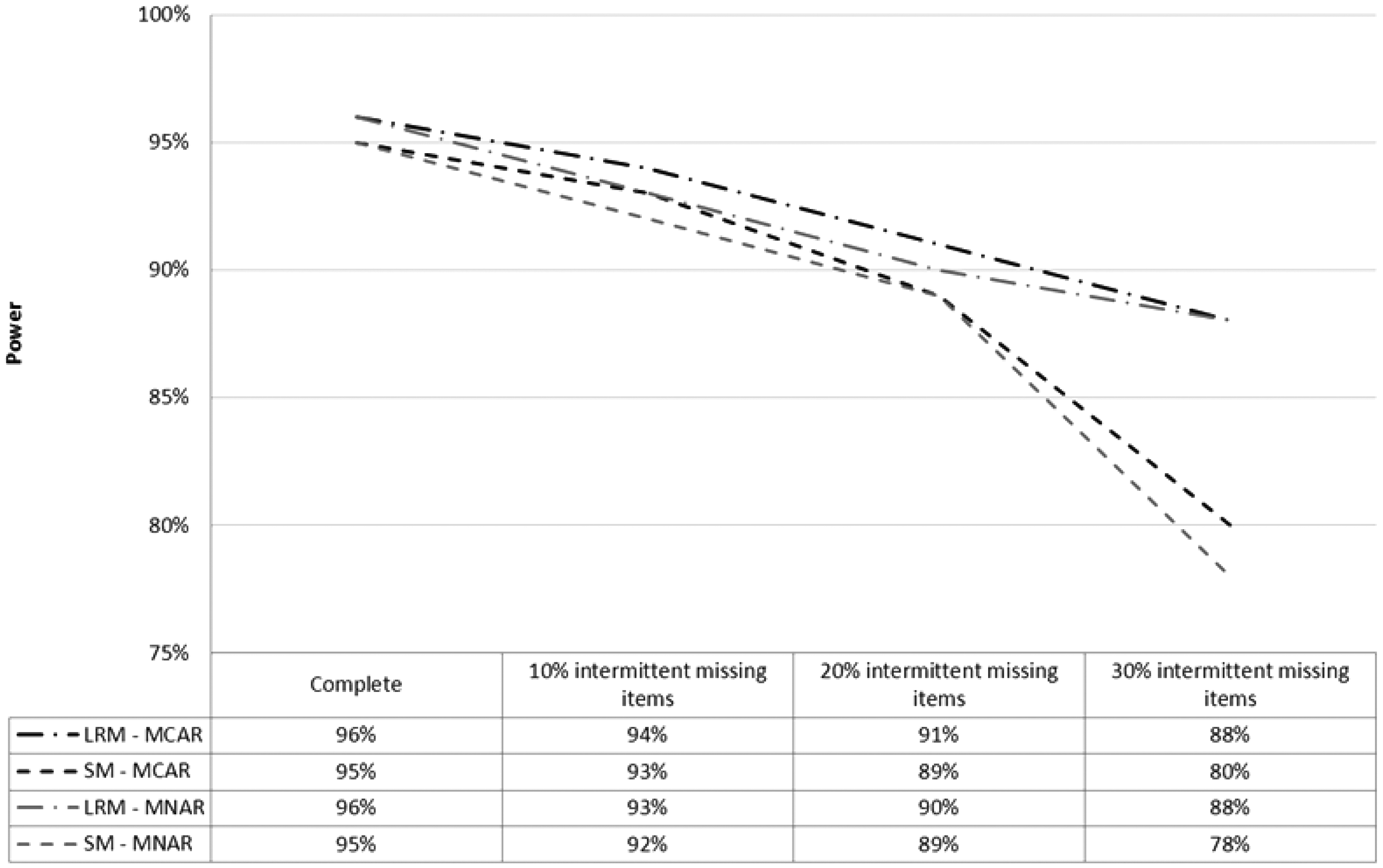 $ρ_{θ} = 0.9$ ), proportion of missing data ( $π = 10 %$ or 20% or 30%) and for complete or MCAR or MNAR ( $ρ_{θ ξ} = - 0.9$ ) data. Analyses performed with an unstructured covariance matrix in SM and LRM methods.

3.3 Supplementary results

Results for datasets obtained with the mechanisms numbered 2, 5 and 8 (Table 1) which depend on items’ parameters (w = 1) and results of datasets obtained with the mechanisms numbered 3, 6 and 9 (Table 1) which take into account the impact of a possible very personal content for one item are not shown. Indeed, the conclusions were very similar regarding type I error, power and time effect estimations when missing items depended on items’ parameters or on the content of items.

4 Illustrative example

This example is based on data of a longitudinal study which has been set up in order to evaluate the evolution of health-related quality of life and coping of breast cancer patients and their caregivers. The aims of this study were to identify if the quality of life and coping strategies of the patients and their caregivers vary over time and if the coping strategies and quality of life of caregivers have an impact on the quality of life of the patients.³⁰ This study took place in Institut de Cancérologie de l’Ouest René Gauducheau (René Gauducheau Cancer Center) in Nantes, France. It is often observed that diagnosis of breast cancer and its treatment instigate stress for patients and their caregivers and that they can use different strategies to cope with this stress. Coping indicates all processes that patients and caregivers use to overcome a negative event that impacts their physical and psychological well-being. Several coping strategies can be employed such as problem-focused coping or emotion-focused coping³¹ to reduce or manage the problem source or the emotional distress, or support-seeking strategies when patients or caregivers look for a social support. Coping was assessed using the ways of coping checklist (WCC) adapted in French by Cousson et al. in 1996.³² The WCC contains twenty seven items with ten items assessing problem-focused coping, nine items for emotion-focused coping and eight items for social support-seeking strategies. A hundred patients were followed at three time points: about two or three weeks after diagnosis (T1), at the end of treatments (T2) and six month after treatments (T3).

The analysis focused on problem-focused coping and Table 6 shows how missing data were distributed for these items.

Table 6.

Distribution of missing data by item for problem-focused coping.

Items	T1		T2		T3
Items	Dropout (%)	Intermittent missing items (%)	Dropout (%)	Intermittent missing items (%)	Dropout (%)	Intermittent missing items (%)
n°1	1	5	14	2	23	0
n°4	1	17	14	1	23	3
n°7	1	13	14	2	23	3
n°10	1	7	14	1	23	0
n°13	1	3	14	2	23	1
n°16	1	29	14	3	23	4
n°19	1	10	14	1	23	3
n°22	1	14	14	5	23	4
n°25	1	27	14	6	23	3
n°27	1	15	14	0	23	4
Mean	1	14	14	2.3	23	2.5

Tables 6 and 7 show the results for illustrative example.

These data were analysed using SM (Proc MIXED in SAS) and LRM (Proc NLMIXED in SAS) methods in order to test whether a time effect exists. The implementation of the two models using SAS is available (Figure 3). Before applying SM, a PMS imputation was used only when the amount of missing items did not exceed 50% for a given patient. Thus, four items maximum were imputed. The computation of the score was made according to the scoring manual: sum of patients’ answers to the 10 items multiplied by 2.5 in order to obtain a score between 0 and 100. For both methods, analyses were performed with a compound symmetry covariance matrix. Indeed, it provided the best fit for these data. Table 7 shows results of these analyses.

Figure 3.

Example of LRM and SM implementations for two times of assessment, ten items with two possible levels of response for eight items (responses 0 or 1 or 2 for items 1; 2; 3; 4; 5; 6; 7 and 8) and only one level for the two other items (responses zero or one for items 9 and 10).

Table 7.

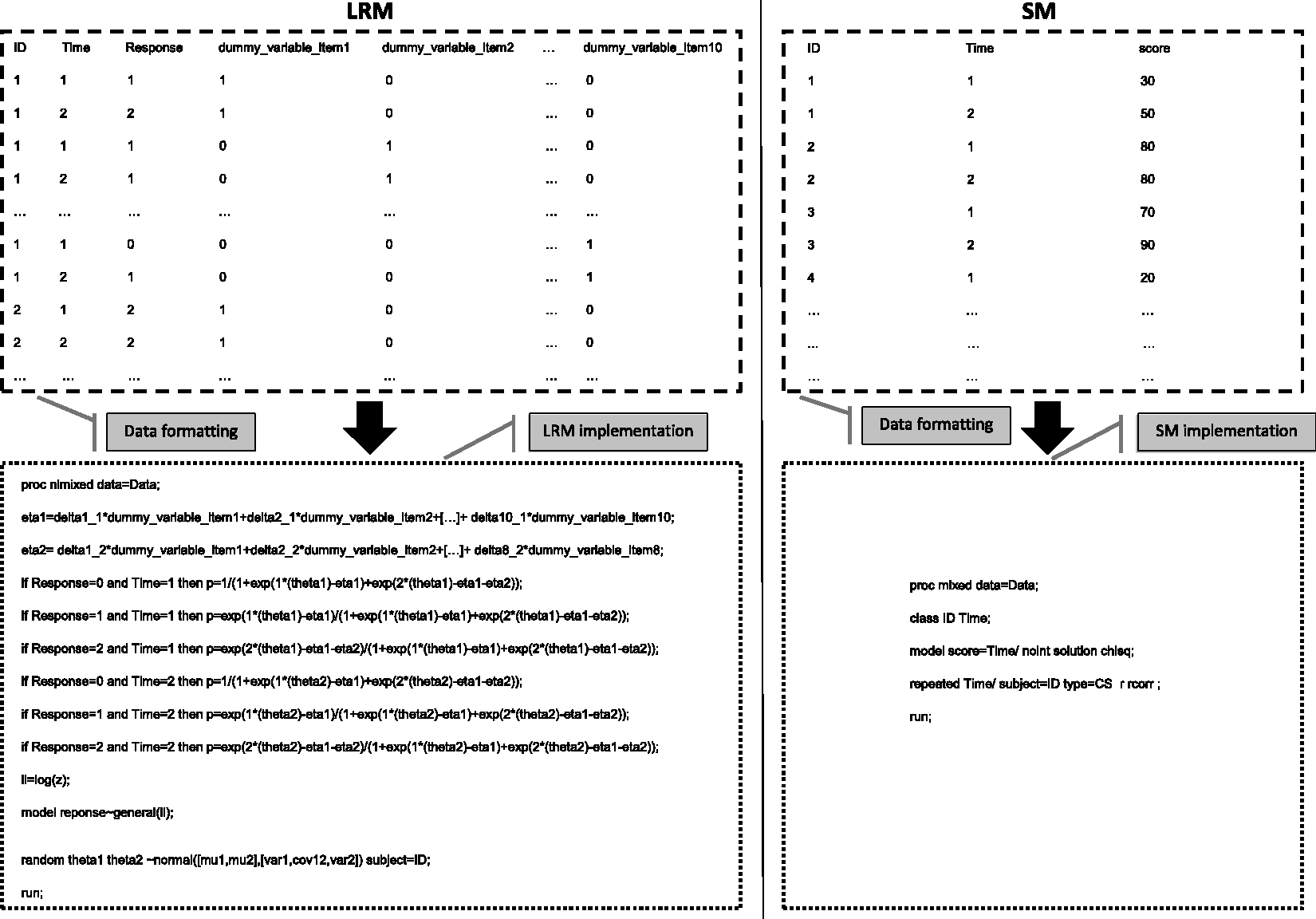
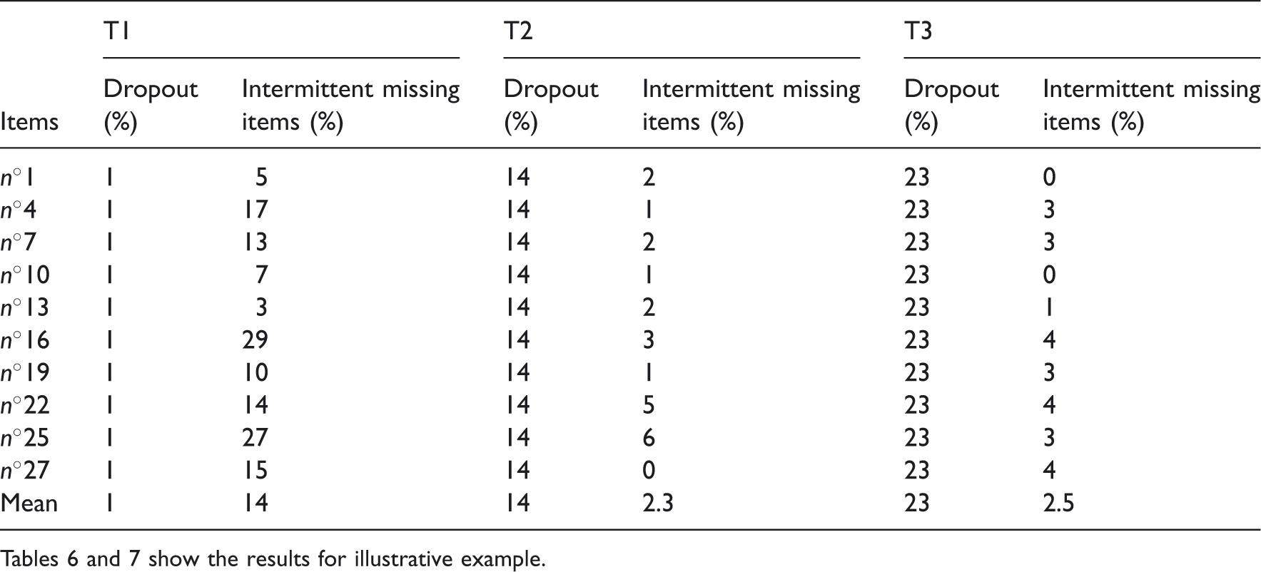
Time effect estimations between time 1 and time 2 ( ${\overset{\land}{d}}_{12}$ ), between time 2 and time 3 ( ${\overset{\land}{d}}_{23}$ ), standard errors (s.e.) and p-values for score mixed model (SM) with personal mean score (PMS) imputation and longitudinal Rasch mixed model (LRM) methods.

SM	LRM
${\overset{\land}{d}}_{12}$	−0.7153	−0.0800
s.e.	0.9476	0.0942
p-value	0.4515	0.3976
${\overset{\land}{d}}_{23}$	0.5274	0.0382
s.e.	0.9851	0.0966
p-value	0.5932	0.6934

Time effects estimations described similar trends for both methods: signs of coefficients were negative between T1 and T2 and positive between T2 and T3. Time effect appeared to be non-significant whatever the method used. Considering the number of patients and the rate of intermittent missing data, these results are in accordance with results obtained in the following case of the simulation study: number of patients N equal to 100, number of items J higher than seven and rate of intermittent missing data ranging from 0% (2.3% and 2.5% for respectively T2 and T3) to 20% (14% for T1).

This example confirms that dropout generates a complete loss of information for both methods, especially between T2 and T3 where the rate of dropout is respectively 14% and 23%. Indeed, no difference between the two methods was noticed between T2 and T3. Moreover, it could be highlighted that the rate of intermittent missing items didn’t exceed 14% (14% for T1, 2.3% for T2 and 2.5% for T3) and that no difference between the two methods could be observed.

5 Discussion

PROs are widely used to measure patients’ perceptions. For this purpose, the evolution of quality of life for instance might be assessed over time and intermittent missing items are an issue that may be problematic if missing items are linked to the patient’s health status. The aim of the present study was to compare CTT and Rasch-based approaches for the detection and quantification of a time effect in the framework of longitudinal PROs with possibly informative intermittent missing items. Two models, each based on CTT and Rasch-based methods, were compared on simulated datasets: SM and LRM models. For the complete datasets, our results were very similar to those obtained by Blanchin et al.:¹⁴ type I errors were maintained to their expected values (5%) and power was almost the same for SM and LRM. Moreover, for the incomplete datasets, the type I error rates were always controlled (close to 5%). In contrast with the conclusions that appeared for dropout missing data in the literature¹⁵ where LRM and SM gave similar and poor results (low power and biased estimations), LRM appeared to perform somewhat better than SM for datasets with intermittent missing items, especially regarding power. Indeed, estimations obtained with LRM were unbiased and power was greater than the one obtained with SM. This study also highlighted a known impact of the type of missing items on the results: values of time effect estimation were more often biased for informative missing items (MNAR data) than for non-informative missing items (MCAR data).

It can be noted that we used a single imputation which is the most often encountered in many manuals (SF-36, QLQ-C30, etc.) for practical reasons.³³ However, it would be interesting to test other methods like multiple imputations in order to have an idea of the impact of other imputation methods in this framework. For LRM, no imputation was necessary and its corresponding power was overall higher than the one obtained with SM. Moreover, in this study, LRM appeared to be an unbiased method whatever the amount of missing items and their informativeness. The difference between the underlying theories for CTT and Rasch-family models might explain these results regarding the impact of intermittent missing items. Indeed, these results might be related to the specific objectivity property of the Rasch model that allows obtaining consistent estimations of the parameters associated with the latent trait independently from the observed items that are used for these estimations.²⁰

The fact that the simulated time effect was assumed to be linear could be considered as a limitation of our study. Indeed, several clinical examples with a non-linear time effect can be quoted. For instance, patients who start chemotherapy often experience a sharp decline of their quality of life which hopefully increases again towards its initial level after some time. As no assumption was made for the estimation of the time effect using SM or LRM, data with a non-linear time effect can be analysed using both methods and the results should be comparable to those obtained in this study. Another limitation could be related to the simulation of dichotomous items which may be remote from reality since polytomous items seem more common in clinical research. However, we could expect similar results for polytomous as for dichotomous items. Indeed, the mechanisms that engender missing items do not depend on the number of items response categories. As a matter of fact, if Rasch-family models are used for analysis, the results obtained might be extrapolated to polytomous items. Indeed, these models also possess the specific objectivity property.

Regarding the intermittent missing items, the MAR process was not simulated. The probability to observe a MAR item depends on observed values but not on unobserved values. It could be possible to simulate intermittent MAR items. As intermittent MAR items are considered as non-informative like MCAR items, the correlation between the latent variable of interest θ and the patient’s propensity of non-response ξ should be simulated at $ρ_{θ ξ} = 0$ (because θ and ξ are independent). Moreover, ξ should depend on the previous observed values. It can be hypothesized that MAR results would be very similar to MCAR results if the information of the previous observed values is taken into account in the analysis.

We considered that the rate of missing items increased with the item parameter’s value but the opposite case could also be imagined. Indeed, it is possible that a patient prefers answering only when items are more appropriate. Moreover, we envisaged the case where a patient with a worse quality of life tends to respond less often to questions because she/he is too tired to answer compared to a patient with a better quality of life. The reverse case could be considered as well and would engender a positive correlation between the latent variable of interest θ and the patient’s propensity of non-response ξ for MNAR items. For instance, a patient with a better quality of life might not see the need to respond to an item because it does not seem appropriate to his/her case. In these scenarios, the rate of missing data would be reduced with item parameter and with the decrease of the quality of life level respectively and we could assume that the methods SM and LRM would perform similarly as in this study. Indeed, the global rate of missing data would not be impacted by these choices of hypotheses and should be quite similar as in our present study.

Our study showed that the LRM model performed better than the SM model regarding power for the analysis of longitudinal PROs with possibly informative intermittent missing items. Indeed, the specific objectivity allowed estimating the latent variable consistently even if the patients did not answer all items. Moreover, these results pointed out the limits of a single imputation like PMS imputation. This study highlighted the interest of the Rasch-based models in clinical research and epidemiology in order to analyse incomplete data from longitudinal PROs studies. Future works with a wider range of IRT models would be interesting.

Footnotes

Declaration of conflicting interests

The author(s) declared no potential conflicts of interest with respect to the research, authorship, and/or publication of this article.

Funding

The author(s) disclosed receipt of the following financial support for the research, authorship, and/or publication of this article: This study was supported by la Ligue Nationale Contre le Cancer.

References

Garcia

Cella

Clauser

. Standardizing patient-reported outcomes assessment in cancer clinical trials: a patient-reported outcomes measurement information system initiative. J Clin Oncol 2007; 25: 5106–5112.

Falissard

. Mesurer la subjectivité en santé: perspective méthodologique et statistique, 2nd ed. Paris: Masson, 2008.

Fairclough

Peterson

Chang

. Why are missing quality of life data a problem in clinical trials of cancer therapy? Stat Med 1998; 17: 667–677.

Bernhard

Cella

Coates

. Missing quality of life data in cancer clinical trials: serious problems and challenges. Stat Med 1998; 17: 517–532.

Little

. Modeling the drop-out mechanism in repeated-measures studies. J Am Stat Assoc 1995; 90: 1112–1121.

Curran

Bacchi

Schmitz

SFH

. Identifying the types of missingness in quality of life data from clinical trials. Stat Med 1998; 17: 739–756.

Curran

Molenberghs

Fayers

. Incomplete quality of life data in randomized trials: missing forms. Stat Med 1998; 17: 697–709.

Fayers

Curran

Machin

. Incomplete quality of life data in randomized trials: missing items. Stat Med 1998; 17: 679–696.

Molenberghs

Kenward

. Missing data in clinical studies, Chichester; Hoboken, NJ: Wiley, 2007.

10.

Little

RJA

Rubin

. Statistical analysis with missing data, 2nd ed. New York: John Wiley, 2002.

11.

Rubin

. Inference and missing data. Biometrika 1976; 63: 581–592.

12.

Schafer

Graham

. Missing data: our view of the state of the art. Psychol Methods 2002; 7: 147–177.

13.

Holman

Glas

CAW

. Modelling non-ignorable missing-data mechanisms with item response theory models. Br J Math Stat Psychol 2005; 58: 1–17.

14.

Blanchin

Hardouin

Neel

. Comparison of CTT and Rasch-based approaches for the analysis of longitudinal patient reported outcomes. Stat Med 2011; 30: 825–838.

15.

Blanchin

Hardouin

Neel

. Analysis of longitudinal patient-reported outcomes with informative and non-informative dropout: comparison of CTT and Rasch-based methods. Int J Appl Math Stat 2011; 24(SI-11A): 107–124.

16.

Lord

Novick

. Statistical theories of mental test scores, Boston: Addison-Wesley Publishing Company, Inc., 1968.

17.

Peyre

Leplège

Coste

. Missing data methods for dealing with missing items in quality of life questionnaires. A comparison by simulation of personal mean score, full information maximum likelihood, multiple imputation, and hot deck techniques applied to the SF-36 in the French 2003 decennial health survey. Qual Life Res 2011; 20: 287–300.

18.

Fayers

Machin

. Quality of life: the assessment, analysis and interpretation of patient-reported outcomes, 2nd edn. Chichester: Wiley, 2007.

19.

Tenenhaus

. Statistique et logiciels: analyse de la variance à effets mixtes utilisation de la Proc MIXED: Mais que reste-t-il à la Proc GLM? La Revue de Modulad 1999; 23: 53–67.

20.

Fischer

Molenaar

. Rasch models: foundations, recent developments, and applications, New York: Springer, 1995.

21.

Glas

Geerlings

van de Laar

. Analysis of longitudinal randomized clinical trials using item response models. Contemp Clin Trials 2009; 30: 158–170.

22.

Davier

Meiser

Rasch models for longitudinal data. In: Carstensen

(ed). Multivariate and mixture distribution Rasch models. Statistics for social and behavioral sciences, New York, NY, Springer, 2007, pp. 191–199.

23.

Zheng

Rabe-Hesketh

. Estimating parameters of dichotomous and ordinal item response models with gllamm. Stata J 2007; 7: 313–333.

24.

Burton

Altman

Royston

. The design of simulation studies in medical statistics. Stat Med 2006; 25: 4279–4292.

25.

Kissane

Patel

Baser

. Preliminary evaluation of the reliability and validity of the Shame and Stigma Scale in head and neck cancer. Head Neck 2013; 35: 172–183.

26.

Cella

Beaumont

Webster

. Measuring the concerns of cancer patients with low platelet counts: the functional assessment of cancer therapy-thrombocytopenia (FACT-Th) questionnaire. Support Care Cancer 2006; 14: 1220–1231.

27.

Bjorner

Petersen

Groenvold

. Use of item response theory to develop a shortened version of the EORTC QLQ-C30 emotional functioning scale. Qual Life Res 2004; 13: 1683–1697.

28.

Holland

Hoskens

. Classical test theory as a first-order item response theory: application to true-score prediction from a possibly nonparallel test. Psychometrika 2003; 68: 123–149.

29.

Sébille

Hardouin

Mesbah

. Sequential analysis of latent variables using mixed-effect latent variable models: impact of non-informative and informative missing data. Stat Med 2007; 26: 4889–4904.

30.

Bonnaud-Antignac

Hardouin

Leger

. Quality of life and coping of women treated for breast cancer and their caregiver. What are the interactions? J Clin Psychol Med Settings 2012; 19: 320–328.

31.

Lazarus

Folkman

. Stress, appraisal, and coping, New York, NY: Springer Pub. Co., 1984.

32.

Cousson

Bruchon-Schweitzer

Quintard

. Analyse multidimensionnelle d’une échelle de coping: validation française de la W.C.C. (ways of coping checklist). Psychologie française 1996; 41: 155–164.

33.

Dempster

Rubin

. Overview. Incomplete data in sample surveys. Vol. II: Theory and annotated bibliography, New York, NY: Academic Press, 1983.