
Abstract
Repeated covariate measurements bring important information on the time-varying risk factors in long epidemiological follow-up studies. However, due to budget limitations, it may be possible to carry out the repeated measurements only for a subset of the cohort. We study cost-efficient alternatives for the simple random sampling in the selection of the individuals to be remeasured. The proposed selection criteria are based on forms of the D-optimality. The selection methods are compared with the simulation studies and illustrated with the data from the East–West study carried out in Finland from 1959 to 1999. The results indicate that cost savings can be achieved if the selection is focused on the individuals with high expected risk of the event and, on the other hand, on those with extreme covariate values in the previous measurements.
1 Introduction
Many epidemiological follow-up studies include covariates, such as blood pressure, cholesterol and weight, that may vary over the time. If only the baseline measurement of these covariates is used, the analysis may suffer from the regression dilution problem,1,2 i.e. the measurement made a long time ago does not anymore predict the disease risk. To avoid this problem, we need to carry out repeated measurements on the time-varying covariates. Conducting these measurements in a large population sample is expensive, and due to budget limitations, we may not be able to select the entire cohort for the new measurement, but only a subset of it. In this article, we study how this subset should be selected in order to estimate the effect of the covariate on survival time as accurately and precisely as possible. We propose the subset to be selected so that a Fisher information-based optimality criterion will be optimized.
The planning of cost-efficient study designs has led to the development of multi-stage (or sequential) designs. In multi-stage studies, the next stage is constructed on the basis of the information obtained from earlier stages under given budget limitations. Multi-stage designs allow us to allocate the sample size optimally between the stages.3,4 Even further, optimality criteria developed originally for design of experiments5,6 can also be applied in observational multi-stage studies. Karvanen et al. explore optimal ways to select a small subset of individuals for expensive genotyping in follow-up studies. 7 Mehtälä et al. consider optimal designs for the measurement times of a binary continuous-time Markov process. 8
The research question outlined above is explored here in a simplified setup with one time-varying covariate and two measurement times using simulated and real data. Several authors have considered general approaches for the joint modeling of survival data and longitudinal covariate data.9–12 The real data come from the Finnish cohorts of the Seven Countries Study 13 carried out in Finland from 1959 to 1999. The objective of The Seven Countries Study was to investigate variation in cardiovascular disease and related risk factors levels. In our example, diastolic blood pressure is the time-varying covariate of interest, and the survival time is considered to be the age at the time of death. With these data, we compare the results corresponding to different selection methods to the situation where every individual is selected for the second measurement.
As we are selecting only a subset of individuals for the new measurement, the majority of individuals do not have this measurement, and thus the handling of missing data plays an important role in the modeling. We study here two alternative ways to deal with the missing data: multiple imputation and a likelihood-based approach with numerical integration. 14
The underlying model is described in Section 2 and the selection criteria are presented in detail in Section 3. In Section 4, we discuss an algorithm, which is used in finding optimal or nearly optimal designs with respect to the chosen criterion. Statistical analysis of data collected during the whole follow-up is described in Section 5, with an emphasis on the handling of missing data. Simulation studies comparing different selection methods are presented in Section 6, followed with results obtained using the real data in Section 7. Finally, Section 8 concludes the paper.
2 Survival model
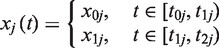
We consider a follow-up study with a predetermined length, where all individuals have a baseline measurement of a single time-varying covariate. The outcome variable is survival time, which is censored at the end of the follow-up. The second measurement of the covariate will be taken halfway through the follow-up. Assume that we cannot afford to remeasure the entire cohort, and therefore have to select a subset of individuals for the second measurement. Here, we study cost-efficient alternatives for the simple random sampling (SRS) in this selection, which is conducted just before the time of the second measurement. The interest lies in the utilization of the baseline measurement information. In addition, the age of an individual may also affect the selection as we are operating with the age as the time axis in our Weibull proportional hazards model.
We start by specifying the survival model, which we need later in defining the selection criteria. Let Y1 = (t1, δ1) denote the survival information at the time of the second measurement, where continuously measured time t1 is censored if the individual is still alive. The status indicator gives δ1 = 1 for the event and δ1 = 0 for censoring. For the second part of the follow-up, we use similar notation Y2 = (t2, δ2).
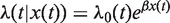
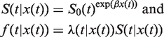
Under the proportional hazards model with a time-varying covariate x(t), the hazard function has the form

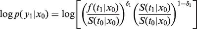
In general form, the survival function and the density function are

3 Selection criteria
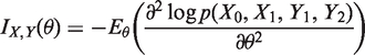
Our main question is, how to select a subset of individuals for the second measurement if only n individuals can be selected? We would like to select a subset which allows parameter β to be estimated as accurately and precisely as possible. Applying the principles of optimal experimental design, the selection criteria are based on the Fisher information matrix of parameters θ = (β, a, b)

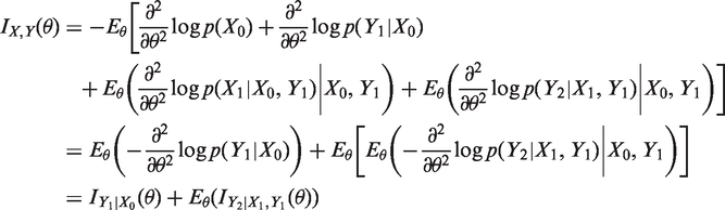
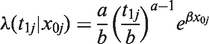
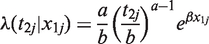
The terms
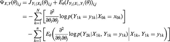
In practice, we replace the first term of equation (1) by observed information
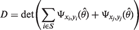
The two selection criteria we will apply are well known criteria from the theory of optimal designs. The methods we will apply in the selection are based on forms of the D-criterion. The D-optimal design is obtained by maximizing the determinant of the information matrix det
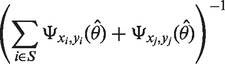
The second method we are using is the Dβ-criterion. Dβ-optimal design is obtained by minimizing the Dβ-criterion, which we define as a diagonal element corresponding to β of the ‘covariance matrix’
The calculation of optimality criteria requires the second order partial derivatives of
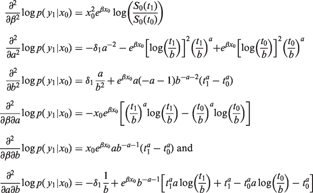
For
From these formulae, it cannot be directly seen what kind of individuals would be included in the Dβ-optimal or D-optimal subsets. Intuitively, we could expect that individuals with extreme covariate values or with high risk of the event would be important for the estimation. In the case of first-order linear regression models, extreme selection of covariate values is optimal, 16 but this does not hold, for example, for quadratic models or binary responses. Extreme selection means selecting individuals with highest and lowest covariate values. Although this method could be applied also in our case, there is no guarantee that it would be optimal in any sense, because we consider a survival model instead of a linear regression model. On the other hand, in survival models, events contain more information than censorings. Intuitively, this means that individuals who are likely to have an event during the follow-up should be selected. Results with simulated and real data in Sections 6 and 7 show how these intuitive principles will be balanced according to Dβ-optimal and D-optimal selections.
4 Finding optimal designs
As the optimal designs of nonlinear models depends on the parameters, we need initial estimates for parameters a, b and β to use optimality criteria in practice. These can be obtained from the data already collected during the follow-up before the time of second measurement and/or from previous studies. For study cohorts of reasonable size, it is not computationally possible to explore all possible subsets of individuals to be selected for the new measurement, but heuristic methods are needed. We use a greedy method 17 where the individuals are selected sequentially one by one to find the optimal subset. This method is also known as the sequential search 18 and is a simplified special case of the Fedorov-Wynn algorithm. 19 The jth individual is selected so that the selection criterion is optimized on the condition that j − 1 individuals have already been selected.
Denote the set of individuals already selected by S. Using Dβ-optimality, the next individual
In general, the selection problem is NP-hard and the greedy method produces only a suboptimal solution. However, the empirical results 7 indicate that the gain from more complicated heuristics may not be large in this kind of design problem.
5 Statistical analysis
5.1 Likelihood-based approach with numerical integration
After the follow-up study, we have data with a large amount of missing data, as only a subset is selected for the second measurement. When that subset is selected using Dβ-optimality or D-optimality, the missingness of that measurement is clearly not missing completely at random (MCAR). However, as the selection depends only on the observed data (X0, Y1), the missing data are missing at random (MAR). Handling missing data plays an important role in the analysis, and for that there are several methods which can be used. In this section, we present a likelihood-based approach and Section 5.2 considers a multiple imputation approach for carrying out the analysis.
Next, we will use the following indexing of individuals. Individuals
The analysis can be carried out with the likelihood-based approach for incomplete data.
20
This requires also the specification of the distributions of the covariate, namely p(x0) and
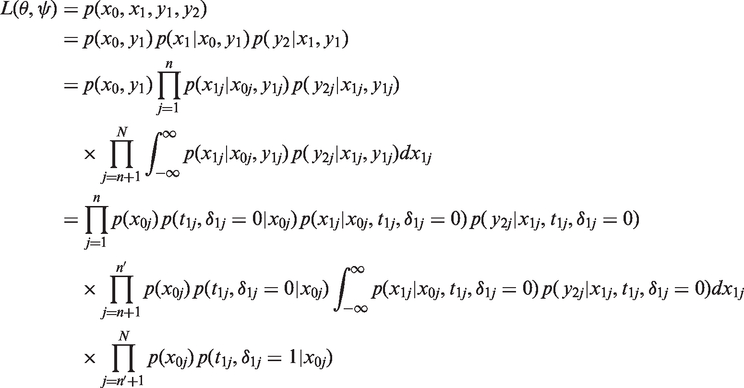
Missing data are treated here as integrals with respect to the missing variable over the support of it. In simple settings with only one covariate, the integrals in the likelihood function can be calculated by numerical integration, which we apply in this paper. If the covariates are categorical variables, the integration would simplify to summation and direct numerical maximization would be feasible and straightforward. In the general setting, methods such as EM-algorithm 21 or Bayesian data augmentation 22 could be used.
5.2 Multiple imputation
Another method we apply in handling missing data is multiple imputation.
23
Now, we do not have to model the marginal distribution
We use a linear imputation model of the form proposed by White and Royston
25

The multiple imputation, using the above imputation model, is carried out in a standard way. 23
6 Simulation study
6.1 Description of the simulation study
Simulation studies were carried out in different settings to explore the performance of the proposed selection methods, namely Dβ-optimality and D-optimality. Simulated data were made to resemble our real data of Section 7 apart from a few exceptions.
We considered a follow-up setting of 20 years with 1500 individuals. A time-varying piecewise constant covariate had the baseline measurement x0 in the beginning and second measurement x1 in the half way of the follow-up. First, the baseline values x0 of the covariate were generated from the normal distribution with mean μ0 = 0 and variance σ2 = 0.02 and the values of second measurement were drawn from the normal distribution conditioned on the baseline measurement with mean μ1 = 0.5x0 and variance
Survival times were simulated from the Weibull distribution depending on the time-varying values of the covariate through the proportional hazards model with regression coefficient β = 3. We chose to use such a large value of β compared to real data, so that the possible effect of covariate stands out in the selection. The parameters of the Weibull distribution were set to shape a = 5.7 and scale b = 28,000 (time scale in days), which roughly equal those estimated from the real data. The survival times of individuals who were alive at the end of the follow-up were censored. The follow-up was conducted at the same calendar time with all individuals, but at each measurement time the ages are not the same for the individuals.
With both narrow and wide age range, 1000 datasets were generated. The numbers of events were on average 101 and 187 during the first half of the follow-up and 222 and 288 during the second half of the follow-up, in datasets with narrow and wide age range, respectively.
6.2 Selection of individuals
The selection of individuals for the second measurement was carried out after 10 years of follow-up by SRS, Dβ-optimality selection and D-optimality selection. Two different sizes, n = 600 and n = 200, of subsets selected for the second measurement were considered. In the case where n = 600, we selected on average 43% with narrow age range and 46% with wide age range of the individuals, who were alive at that moment. The corresponding numbers in the case where n = 200 are 14% and 15%, respectively.
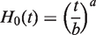
Before presenting the results obtained with different selection methods, we examine what kind of individuals are selected according to Dβ-criterion and D-criterion, in other words, who are most important to remeasure. Figure 1 shows the selection order for any n up to 600, when the selection is based on the Dβ-optimality. The order is, of course, irrelevant when we analyze the data. The selection seems to prefer extreme baseline covariate values, but also the age of an individual has an effect. With the wide age range, the age is the more important factor in the selection than with the narrow age range.
Selection order of individuals to be remeasured for any n up to 600 using Dβ-optimality and simulated data. The left panel shows the order for data with narrow age range and the right panel is for the wide age range. Each point corresponds to one individual: the brightness (color in the online version) shows the age of the individual at the time of the selection, the vertical axis shows the value of the baseline covariate and the horizontal axis shows the round when the individual was selected in the greedy algorithm. The histograms on the right vertical axes show the distribution of the covariate in the entire cohort. With the wide age range, the minimum age selected is 41 years although the minimum age in the cohort is 35 years.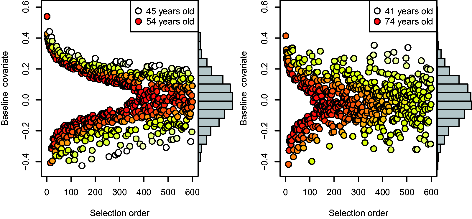
From Figure 2, we see that using the D-optimality leads to rather different kind of selection compared to Dβ-optimality. With the narrow age range, during the first few dozens of selection rounds, the D-optimal selection is focused on individuals with high covariate values and high age. However, the age has a greater effect on selection than with Dβ-optimality, especially when we consider the wide age range.
Selection order of individuals to be remeasured for any n up to 600 using D-optimality and simulated data. The left panel shows the order for data with the narrow age range and the right panel is for the wide age range. Each point corresponds to one individual: the brightness (color in the online version) shows the age of the individual at the time of the selection, the vertical axis shows the value of the baseline covariate and the horizontal axis shows the round when the individual was selected in the greedy algorithm. The histograms on the right vertical axes show the distribution of the covariate in the entire cohort.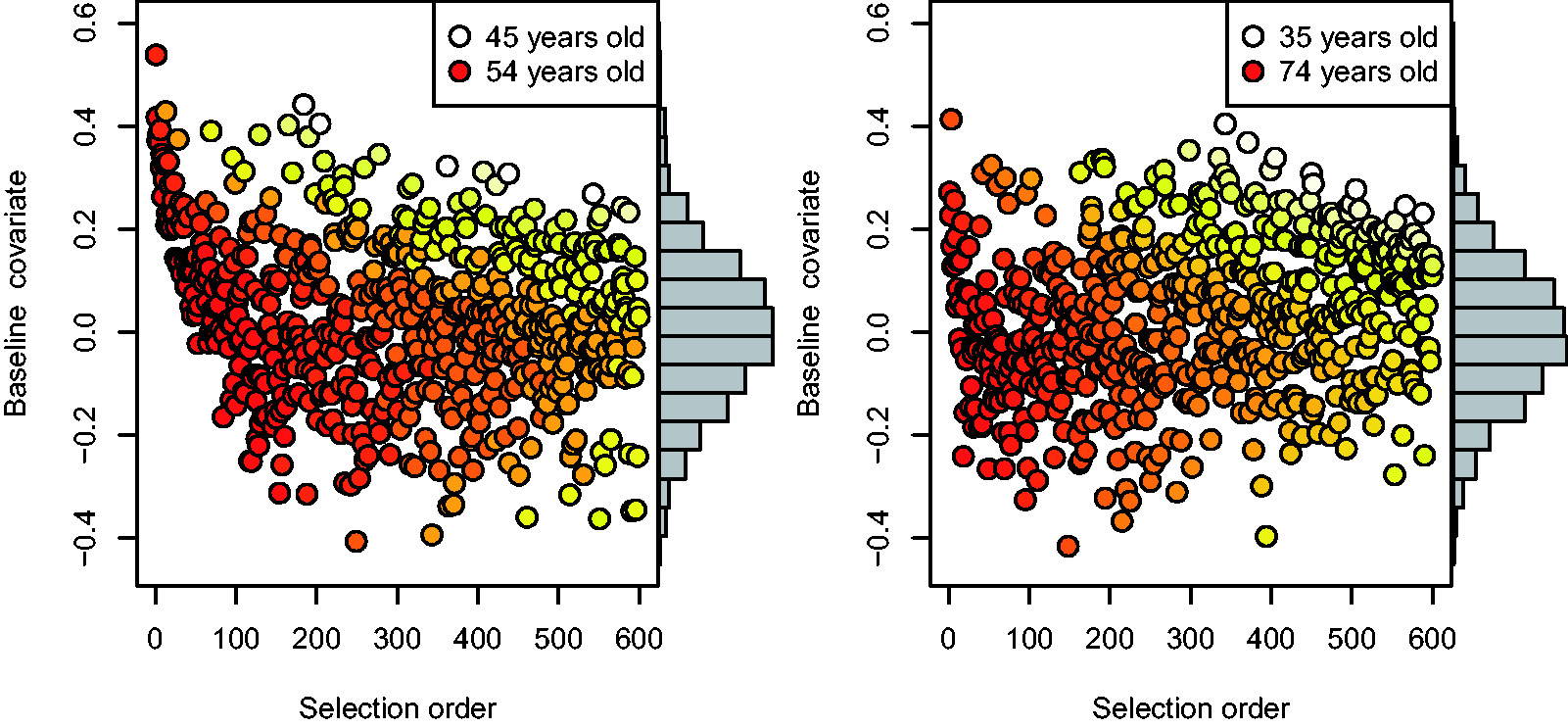
6.3 Analyses with different designs
The aim of the selections illustrated in Figures 1 and 2 is to find the subset which would lead to as reliable as possible estimation of parameter β in our Weibull proportional hazards model. All analyses were carried out with the R statistical software.
26
With multiple imputation, the
Simulation results for different designs using numerical integration.
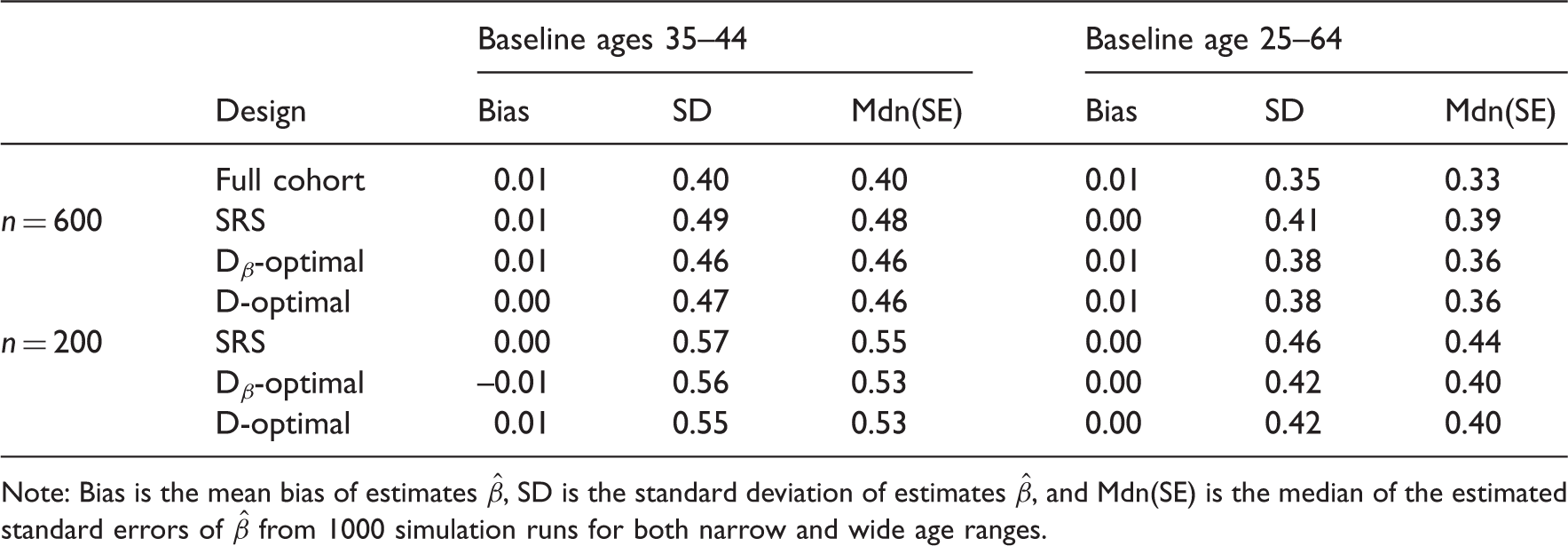
Note: Bias is the mean bias of estimates
Simulation results for different designs using multiple imputation.
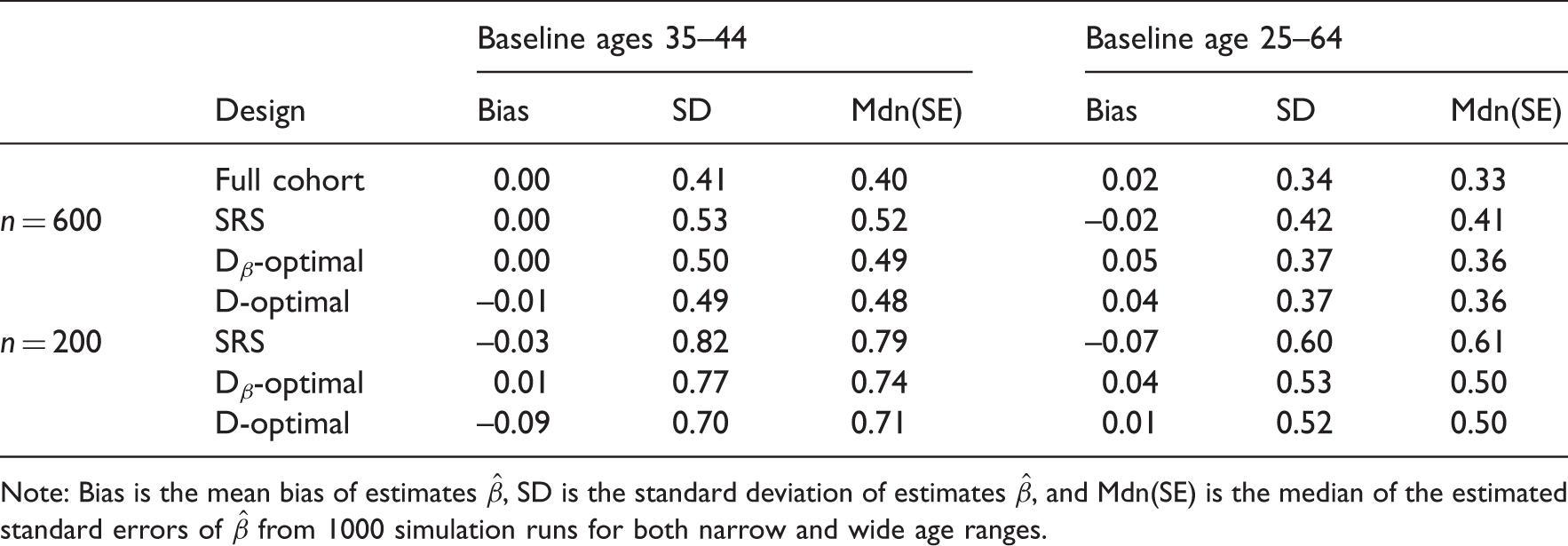
Note: Bias is the mean bias of estimates
In Tables 1 and 2, the standard errors and deviations seem to be quite consistent when n = 600, especially with the wide age range. Nevertheless, when we compare the results of multiple imputation and numerical integration with narrow age range in the case where n = 200, we see that multiple imputation produces clearly greater standard errors and deviations. Furthermore, in this setting the D-optimality seems to perform better than Dβ-optimality. This is, however, a problem related to multiple imputation, since theoretically the Dβ-optimal design cannot give larger standard error for
7 Results for the east–west study
Data from the Finnish cohorts of the Seven Countries Study are used. The Seven Countries Study was initiated in the late 1950s to study variation in cardiovascular disease and related risk factors levels. 13 The Finnish cohorts (N = 1711) included all men born between 1900 and 1919 in two geographically defined areas, one in eastern and the other in south-western Finland, from which comes the name East–West study. The baseline survey was conducted in 1959 and re-examinations in 1964, 1969, 1974, 1984, 1989, 1994, and 1999.30,31 The cohorts were followed up for mortality until the end of 2010. In these analyses, data on re-examination from 1964 and 1974 and information on the age of death are used.
We use only a part of the data so that we consider the measurement of the year 1964 as the baseline measurement, 1974 as the year of the second measurement and 1984 as the end of the follow-up, when censoring is carried out. As a time-varying covariate, we use diastolic blood pressure, which is logarithmic and centered in the analyses. Survival time is considered to be the age at the time of death. After removing individuals who were already dead before the measurement of the year 1964 and who do not have observations of diastolic blood pressure, we have 1501 eligible individuals for our study. In this setting, we have 354 events in the first half and 424 events in the second half of the follow-up.
The selection order with Dβ-optimality and D-optimality can be seen in Figure 3. Dβ-optimality seems again to prefer extreme covariate values and at a fixed value of covariate, older individuals are selected first. In D-optimality, the age is clearly a more important factor in the selection. All in all, the selection with the East–West data looks very similar compared to one with the simulated data, which could have been expected, because the simulated data were made to resemble these real data.
Selection order of individuals to be remeasured for any n up to 600 in the East–West data using Dβ-optimality (left panel) and D-optimality (right panel). Each point corresponds to one individual: the brightness (color in the online version) shows the age of the individual at the time of the selection, the vertical axis shows the value of the baseline covariate and the horizontal axis shows the round when the individual was selected in the greedy algorithm. The histograms on the right vertical axes show the distribution of the covariate in the entire cohort.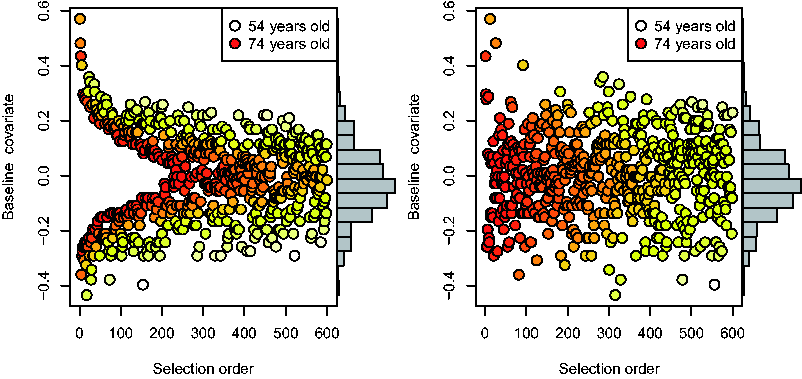
Results with the East–West data for different designs using multiple imputation.
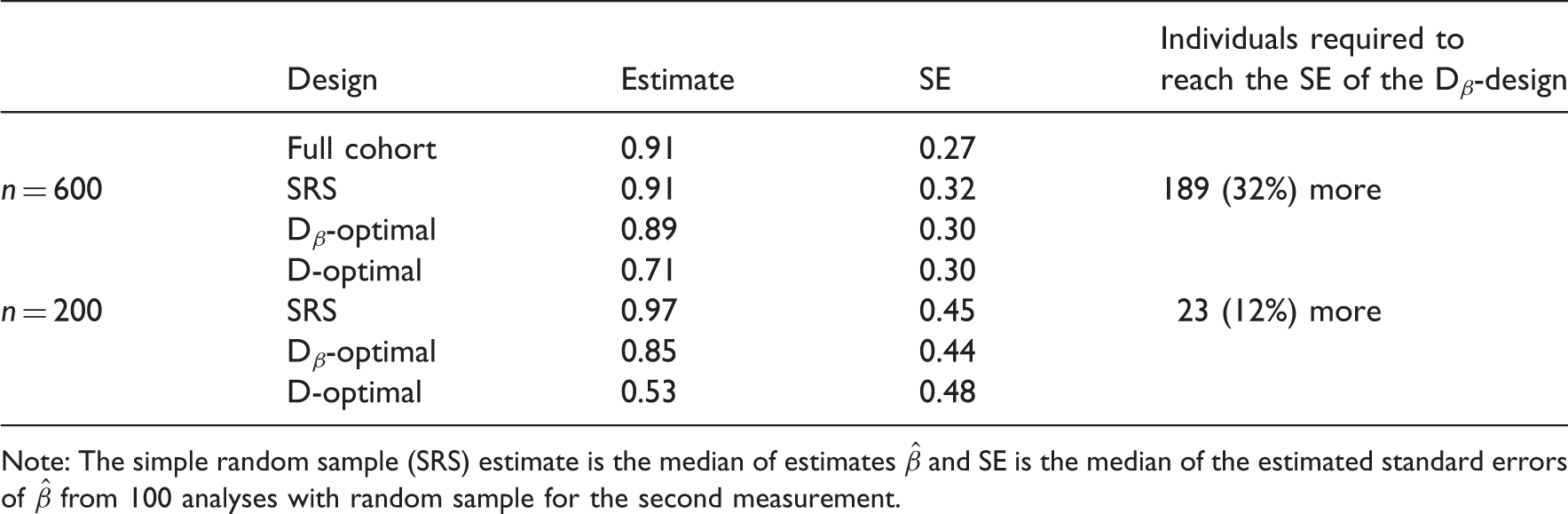
Note: The simple random sample (SRS) estimate is the median of estimates
It is worth noting that the gain from the optimal designs is free of charge once the selection procedure has been implemented. Comparing the designs with n = 600, we approximate that reducing the standard error of the SRS-design to the level of the Dβ-optimal design would require about 189 more individuals to be remeasured. That is, the efficiency of the SRS-design is 75% in this comparison. This kind of amount of measurements would create notable additional costs in epidemiological studies, like the East–West study. In the case where n = 200, approximately 23 more individuals are required in the SRS-design to reach the standard error of the Dβ-design, which means that the SRS has here the efficiency of 90%.
8 Conclusion
Limited resources lead us to investigate the cost-effectiveness of study designs. In this paper, we considered the selection of individuals for the often costly re-examination of a time-varying covariate in a follow-up study. Two different Fisher information-based optimality criteria, Dβ-optimality and D-optimality, were applied and compared to the SRS using simulated data and real epidemiological follow-up data.
The selections carried out according to the optimality criteria indicate that individuals with extreme baseline covariate values and high age would be most important to remeasure. The criteria balance differently between these characteristics: Dβ-optimality stresses the extremity, whereas D-optimality prefers old individuals. With both criteria, age is the more important factor in the selection when the age range of individuals is wide than when the age range is narrow. Results from the analyses with different designs show that when handling missing data with multiple imputation or numerical integration, the precision is usually better for the optimal selections than for the SRS. No clear differences between the two optimal selections were observed. Numerical integration looks better than multiple imputation according to the simulation results, but from the real data we have learned that it may be sensitive to the model assumptions.
When the proportion of the missing data is large, the estimation may be sensitive to the model misspecification. 32 However, it should be emphasized that the model used for the optimal selection may be different from the model used in the analysis. After the second measurement, it is possible to check the validity of the distributional assumptions and change the model if needed.
The future work will consider more complicated designs where several repeated measurements will be carried out on several covariates. The current work forms a basis for these extensions.
Footnotes
Acknowledgements
The authors are grateful to an anonymous referee for valuable comments. We also thank Jukka Nyblom, Harri Högmander, Jouni Helske and Satu Helske for helpful comments and suggestions.
Declaration of conflicting interests
The author(s) declared no potential conflicts of interest with respect to the research, authorship, and/or publication of this article.
Funding
The author(s) disclosed receipt of the following financial support for the research, authorship, and/or publication of this article: The research of the first author was supported by the Emil Aaltonen Foundation.