The attributable fraction is a widely used measure to quantify the public health impact of an exposure on an outcome. It was originally proposed for binary outcomes, but attributable fraction estimators have also been proposed for time-to-event outcomes. In this note, we consider an estimator which was proposed by Benichou (Stats Methods Med Res, 2001) and is supposed to estimate the cohort attributable fraction, i.e. the number of events that would have been prevented in the cohort during follow-up, if the exposure would hypothetically have been eliminated. We show that this estimator is only valid under certain assumptions, which are often likely to be violated in practice. We further argue that the cohort attributable fraction may not be of substantial scientific interest in the first place. We propose a potentially more relevant measure of attributable fraction in cohort studies; the baseline attributable fraction. We show how the baseline attributable fraction can be conveniently estimated in Cox proportional hazards models.
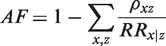
The attributable fraction (AF; also known as the attributable risk) is a widely used measure to quantify the public health impact of an exposure on an outcome. It was originally defined for binary outcomes as the proportion of outcomes that would be eliminated in the population if the exposure was hypothetically eliminated.1 In observational studies, consistent estimation of the AF typically requires appropriate confounder adjustment. Benichou2,3 gave an overview of various adjusted estimators, including the Mantel–Haenszel estimator, the weighted-sum estimator, and the model-based estimator. The latter is based on the following algebraic rearrangement of the AF
In this expression, the sum is taken over all joint levels of the exposure X and the adjustment covariates Z. is the conditional risk ratio for level x of the exposure, given level z of adjustment covariates, and is the population proportion with levels and among the cases (subjects who have the outcome). The model-based estimator can be used for both case–control studies and cross-sectional studies with binary outcomes, by replacing with the sample proportion of cases with levels and , and by replacing with an estimate obtained from a regression model; in case–control studies, this risk ratio has to be approximated by the corresponding odds ratio.
Benichou2,3 claimed that the model-based estimator can be adapted to cohort studies with right censored time-to-event outcomes, by replacing with an estimate of the adjusted (hazard) rate ratio obtained from a Poisson or Cox regression. However, he provided no formal justification for this claim. Furthermore, he did not clarify what to replace with when the outcome is no longer binary. We made a survey of recent literature and found that the cohort adaption of the model-based estimator proposed by Benichou2,3 has been used in many studies.4–11 In all these studies, was replaced with the sample proportion with levels x and z among those who were observed to experience the event before end of follow-up; we refer to the resulting estimator of the AF as the “cohort-adapted estimator.” Without exception, the authors of these studies appear to have interpreted the cohort-adapted estimator as estimating the proportion of events that would have been eliminated in the cohort during follow-up, if the exposure had been eliminated; we refer to this proportion as the “cohort attributable fraction” (CAF). In this note, we show that the cohort-adapted estimator only estimates the CAF under the following two assumptions: (1) the cumulative incidence is small during the whole follow-up, and (2) there is no censoring, apart from administrative censoring at the end of follow-up. When either of these assumptions is violated, the cohort adapted estimator does not estimate the CAF and may have no meaningful interpretation. We further argue that even if both these assumptions hold, the CAF may not be of substantial scientific interest. We propose a potentially more relevant measure of attributable fraction in cohort studies, the baseline attributable fraction (BAF). We show how the BAF can be conveniently estimated in cohort studies, using Cox proportional hazards models.12 Our estimator does not require the two aforementioned assumptions required by the cohort-adapted estimator.
The paper is organized as follows. In Section 2, we show that the cohort-adapted estimator only converges to the CAF under the aforementioned two assumptions. In Section 3, we argue that the CAF may not be a relevant measure of attributable fraction in the first place, and we propose the BAF as a potentially more relevant measure. In Section 4, we show how the BAF can be conveniently estimated in Cox proportional hazards models. In Section 5, we carry out a small simulation study to demonstrate the consistency of our proposed estimator. In Section 6, we present an application to real data.
2 The underlying assumptions of the cohort-adapted estimator
We first introduce some notation. We consider a binary exposure X, with levels 0 and 1 for “unexposed” and “exposed,” respectively. We let T denote the random time to event. We assume that the event of interest is “absorbing,” so that when the event occurs the individual is no longer part of the cohort, e.g. when the subject dies. We let τ denote the end of follow-up. To begin with, we assume that there is no censoring apart from administrative censoring at the end of follow-up.
We will throughout assume that the conditional log hazard function, given X and adjustment covariates Z, follows the Cox proportional hazards (PH) model
where is the unspecified baseline hazard function. The Cox PH model is not crucial for any of the arguments that we make but simplifies the exposition. In this section, we are only concerned with asymptotic properties (e.g. bias) of the cohort-adapted estimator and not its finite sample behavior. Thus, to further simplify the exposition we will assume that the cohort is “infinitely large”, so that we do not need to bother about sampling variability. Under the model in (1), the cohort-adapted estimator can be expressed as
where is the proportion in the cohort with levels and among those who experience the event during follow-up.
To relate the cohort-adapted estimator to the CAF, we need a formal definition of the latter. Using standard potential outcome notation13,14 we let T0 denote the counterfactual time to event that would have been observed for a given subject, had that subject been unexposed. We let denote the factual proportion of events that occurs at or before time t in the cohort (i.e. the cumulative distribution function at ), and we let denote the counterfactual proportion of events that would occur at or before time t in the cohort, had everybody in the cohort been unexposed. In this notation, the CAF is equal to
For instance, if 20% of all subjects in the cohort factually experience the event before the end of follow-up, but only 5% would experience the event had everybody been unexposed, then the CAF equals .
In randomized trials, exposed and unexposed are exchangeable so that is equal to the proportion of subject who would experience the event before end of follow-up among those factually unexposed, i.e. . In observational studies, can be estimated by adjusting for covariates, if these are appropriately selected and sufficient for confounding control. To determine whether a particular set of covariates is sufficient or not is a difficult problem, and one that typically requires strong subject matter knowledge. This problem of covariate selection is beyond the scope of this paper; we proceed by assuming that we have measured a set of covariates Z which is sufficient for confounding control. Under this assumption, is equal to , where the outer expectation is taken over the marginal distribution of Z.15,16 It follows that the CAF can be rewritten as
which is equal to the (asymptotic limit of the) cohort-adapted estimator. Note the approximation just before the last equality in the derivation; this approximation is only valid if the cumulative incidence is small, in which case is approximately equal to . Thus, the cohort-adapted estimator does indeed approximately estimate the CAF, provided that the cumulative incidence is small throughout follow-up.
To see that the cohort-adapted estimator can be severely biased if the cumulative incidence is large, consider the case when the event of interest is death and the follow-up is infinite; . In this case, the CAF is equal to 0, since (eventually, everyone dies). However, the cohort-adapted estimator equals , which may be far from 0, unless (i.e. unless the exposure has no effect).
We next consider the impact of random right censoring. Let C denote the random time to right censoring, so that for each subject we observe the event if .17 In the presence of random censoring, we cannot observe , but have to replace this proportion in the cohort-adapted estimator with , that is, with the proportion in the cohort who are exposed among those who are observed to experience the event during follow-up. To see that this modification may induce bias, suppose that the censoring is heavy, so that a large fraction is censored early during follow-up. Those who contribute to will then mainly be those who die early. If there is an association between the exposure and the time to death, then there will be an overrepresentation of exposed subjects in this group, as compared to those who die before end of follow-up. This implies that , so that the cohort-adapted estimator becomes biased upwards. We note that this bias will be present even if C is completely independent of both X, Z, and T.
3 The baseline attributable fraction
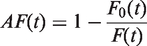
Many cohort studies have relatively long follow-up, or relatively high baseline hazard, so that the assumption of small cumulative incidence is not tenable. Censoring, either random or nonrandom, is also commonly present. Thus, the cohort-adapted estimator may often be biased, as an estimator of the CAF. Recently, methods have been proposed which can be used to consistently estimate the CAF even if the cumulative incidence is not small and random censoring is present.18,19 However, it can be questioned whether the CAF is a relevant measure of attributable fraction in the first place. The problem is that the CAF depends on the actual follow-up time τ in a rather arbitrary fashion. In particular, as already noted, the CAF is 0 when the event of interest is death and τ is sufficiently large, since eventually everyone dies regardless of whether we are able to eliminate the exposure or not. To bypass this problem, one could instead present (an estimate of) the whole AF function
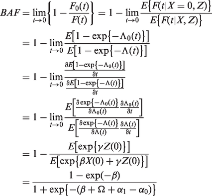
which measures the proportion of events that would have been eliminated in the cohort as a function of time, if the exposure had been eliminated.18,19 A strength of the AF function is that it preserves the time dynamics of the cohort study by not summarizing the exposure impact into a scalar measure. This strength may also be a weakness though; it is typically more difficult to communicate and interpret a (possibly complicated) function than a single number. If we wish to summarize the exposure impact by one scalar measure, then we may think of various alternatives. One option may be the maximum value , which provides a global upper bound on the AF function. This measure may be relevant in scenarios where the AF function starts and remains at zero for some time after the study start before increasing, for instance when the exposure is (absence of) a treatment which takes a while to build up and become effective. Another option may be the limit value , which measures the proportion of events that would have been eliminated in the cohort in the long run, if the exposure had been eliminated. This measure may be relevant when the event of interest is, in contrast to death, not inevitable in the long run, for instance when the event is the occurrence of a particular disease.
We will focus on the limit value , which measures the proportion of events that would have been eliminated during a short (infinitesimal) period of time immediately after baseline in the cohort, if the exposure had been eliminated; we refer to this measure as the “baseline attributable fraction” (BAF). The BAF coincides with the maximum value of the AF function when the AF function is monotonically decreasing. An attractive feature of the BAF is that it does not only apply to the cohort but also to the population from which the cohort was drawn. This is not generally true for other summaries of the AF function, since the characteristics of a (closed) cohort often change and diverge from the characteristics of the source population over time, as subjects gradually drop out from the cohort due to death or for other reasons. At baseline though, the cohort is still guaranteed to be representative for the source population, and thus the BAF can be interpreted as the proportion of events that would have been eliminated during a short period of time in the source population, if the exposure had been eliminated. We emphasize that the BAF may not always be a relevant measure of attributable fraction, e.g. when the exposure has no short-term effect, so that the BAF is equal to 0 even though the exposure may have a long-term effect. However, in many scenarios, in particular when the effect of the exposure is relatively constant over time, the BAF summary measure may offer a useful compromise between relevance and parsimony.
Under Cox PH models, the BAF has a simple and instructive expression. Consider the following Cox PH model, which generalizes the model in (1) in that it allows for both X and Z to vary over time
We emphasize that even though this model allows for the exposure to vary over time, it assumes that the effect of the exposure () is constant over time. Let denote the proportion exposed at baseline, and let denote the log odds of being exposed at baseline. Let and denote the log of the mean of , for the exposed and unexposed at baseline, respectively, i.e. . If Z is sufficient for confounding control, then it can be shown (see Appendix 1) that under the model in (3), the BAF can be written as
To gain some intuition for this expression, it is useful to study how the RHS of (4) depends on the causal effect of X on T, on the proportion exposed at baseline, and on the strength of confounding. It is easy to show that the RHS of (4) increases with both β and , and equals 0 if either or . This is reasonable; if the exposure has no effect on the outcome (so that ) or if nobody is exposed (so that ), then no events can be attributed to the exposure. When β goes to ∞, the RHS of (4) goes to 1. This is also reasonable; if the exposure has a strong effect on the outcome, then most of the events could be attributed to the exposure. The term depends on the strength of confounding, and equals 0 if either Z and T are independent (so that or Z and X are independent (so that does not depend on ).
4 Estimation of the BAF under Cox PH models
The Cox PH model in (3) can be fitted to data with standard software to obtain estimates and . Subsequently, the log of the sample means of and can be used as estimates and , respectively. The sample log odds of being exposed at baseline can be used as an estimate . Finally, the estimates can be plugged into (4), to obtain an estimate .
To assess the statistical uncertainty in , it is desirable to derive its asymptotic distribution. Using the multivariate delta method,20 we have that has an asymptotic normal distribution with variance , where g is the column vector of derivatives of BAF with respect to , and is the asymptotic variance–covariance matrix of . By differentiating the BAF with respect to , we have that
and
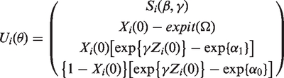
Define . To derive we note that solves the estimating equation , where
is the estimating equation contribution from subject i, and is the Cox partial likelihood score contribution from subject i. We note that the ’s are not independent since the same subject may appear in several risk sets during follow-up. However, it follows from results in the Appendix of Lee et al.21 that this dependence may be asymptotically ignored. Treating the ’s as independent it then follows from standard results on estimating equations22 that has an asymptotic normal distribution with variance–covariance matrix equal to , where and . Define and let denote the submatrix of corresponding to the elements of . We then have that . Estimates of g, h, and can be obtained by replacing the true value of θ and the population moments in with the estimate and the corresponding sample moments.
The derivation of outlined above assumes that the subjects are independent. Often, this assumption may be violated due to clustering, e.g. in studies of siblings or twins. When the clusters are independent, it is easy to correct for dependencies within clusters. Let denote the estimating equation contribution from subject j in cluster i, and define . With this minor modification, the ’s are now independent and is equal to as before.21
5 Simulation study
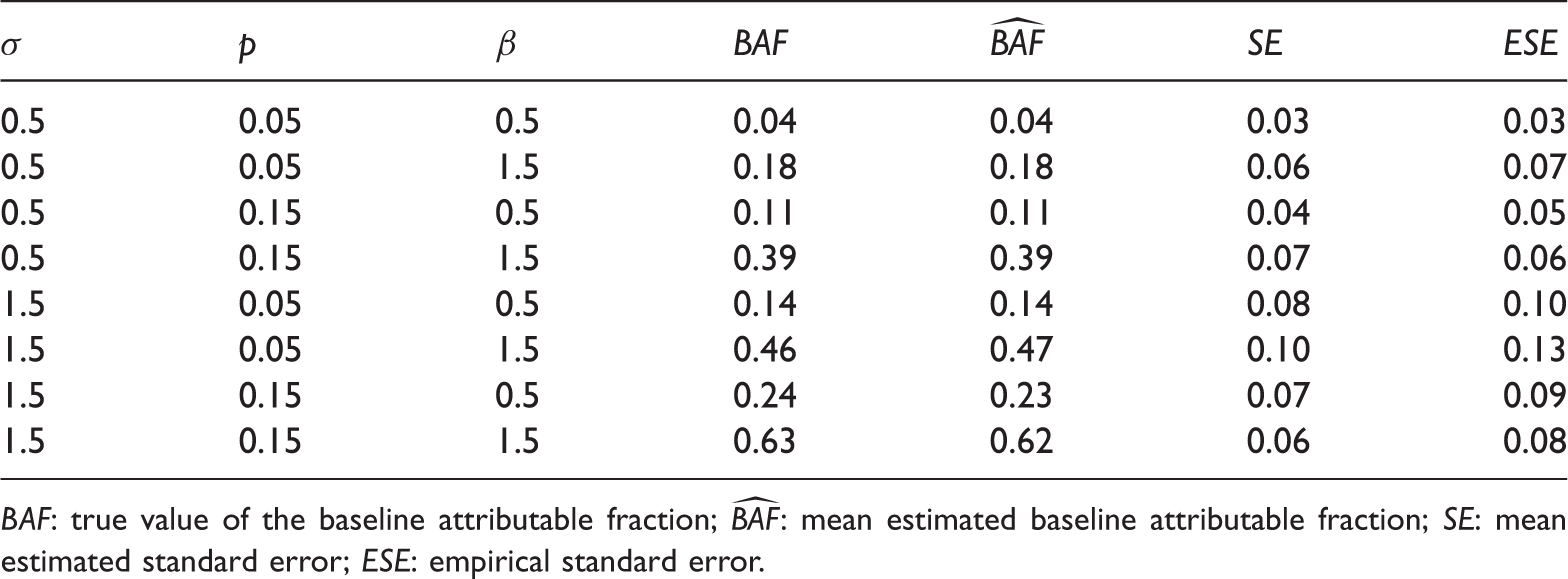
To investigate the finite sample properties of the proposed methods, we carried out a small simulation study. In all simulated scenarios, we generated a time-stationary covariate Z from a normal distribution with mean 0 and standard deviation σ. We generated a time-stationary exposure X from the logistic model . For each simulated scenario, ω was set to achieve a desired value of p, as described below. We generated survival times T from the Cox proportional hazards model in (1), with . We generated random censoring times C from the same conditional distribution as T, given X and Z. Under this scheme, C is associated with X and Z, but conditionally independent of T, given X and Z. The marginal (over X and Z) censoring rate is 50%. From this model, we generated 1000 samples of independent subjects, for each of the eight possible parameter combinations of , , and . For each sample, we estimated the BAF and its standard error using the method described in Section 4. Table 1 displays the mean (over the 10,000 samples) estimated BAF () together with the true value (), and the mean estimated standard error () together with the empirical standard error () for each scenario. We observe that the mean estimated BAF is close to the true value and that the mean estimated standard error agrees well with the empirical standard error, for all scenarios.
Simulation results for estimation of the BAF, for 1000 samples of independent subjects.
σ
p
β
0.5
0.05
0.5
0.04
0.04
0.03
0.03
0.5
0.05
1.5
0.18
0.18
0.06
0.07
0.5
0.15
0.5
0.11
0.11
0.04
0.05
0.5
0.15
1.5
0.39
0.39
0.07
0.06
1.5
0.05
0.5
0.14
0.14
0.08
0.10
1.5
0.05
1.5
0.46
0.47
0.10
0.13
1.5
0.15
0.5
0.24
0.23
0.07
0.09
1.5
0.15
1.5
0.63
0.62
0.06
0.08
BAF: true value of the baseline attributable fraction; : mean estimated baseline attributable fraction; : mean estimated standard error; : empirical standard error.
6 Real data illustration
In this section, we present an application to real data, borrowed from Carlsson et al.23 These authors aimed to study the association between body mass index (BMI) and mortality. Their cohort data comprise 44,258 Swedish same-sex twins, of which 16,793 are monozygotic (MZ) and 27,465 are dizygotic (DZ). All twins filled in a questionnaire in 1967 or 1972 on lifestyle factors, health, height, and weight. Death records were obtained by linkage to the National Causes of Death Registry for the years 1972–2004. The authors stratified the analysis on zygosity and sex, and controlled for smoking in the statistical models.
We reanalyzed the Carlsson et al data as follows. Baseline (i.e. ) was defined as the date when the questionnaire was filled in. BMI was dichotomized into BMI ≤ 25 (unexposed) and BMI > 25 (exposed). The BAF was estimated for the DZ and MZ twins separately, controlling for smoking, sex, and age at baseline. Clustered standard errors were computed to account for the correlation between twins in the same pair, as described in Section 4. These standard errors were subsequently used to construct 95% Wald confidence intervals (CIs). For the DZ twins we obtained = 0.06, with 95% CI ranging from 0.02 to 0.10. For the MZ twins, we obtained = 0.07, with 95% CI ranging from −0.11 to 0.25. These results indicate that around 6–7% of all deaths would have been eliminated in this cohort of DZ/MZ twins, immediately after baseline, if all twins would have had BMI ≤ 25 at baseline.
Before leaving this example, we take the opportunity to note that attributable fractions are conceptually difficult when the exposure of interest is BMI. The reason is that it may not be entirely clear what it means to be “unexposed,” e.g. to have BMI ≤ 25. Clearly, there are many ways to reduce BMI; we may for instance drastically reduce the amount of body fat or the amount of muscles on everybody. These two hypothetical interventions may both render everybody “unexposed,” but the mortality rates under these interventions may be very different. Thus, unless we make the exposure definition more precise, we may consider the attributable fraction as somewhat ill-defined. We therefore conclude by recommending that researchers who wish to study the public health impact of obesity should make an effort to make their definition of obesity/nonobesity as precise as possible, in order to reduce vagueness in the research question being posed.
7 Discussion
We have studied the commonly used cohort-adapted estimator, which is supposed to estimate the CAF. We have shown that this estimator relies on two assumptions, which are often not tenable in practice. We have argued that the CAF may not be a relevant measure of public health impact in the first place, and we have proposed to use the BAF instead. We have shown how the BAF can be conveniently estimated in Cox proportional hazards models.
A major obstacle for practitioners who wish to use new methodology is often the lack of implementation in standard software. To facilitate the proposed methods, we have written a convenient R-function, which implements the BAF estimator proposed in Section 4. This R-function is available at http://www.meb.ki.se/personal/arvsjo/, and can be obtained from the author upon request. We describe its usage in the Appendix 1.
Footnotes
Declaration of conflicting interests
The author(s) declared no potential conflicts of interest with respect to the research, authorship, and/or publication of this article.
Funding
The author(s) disclosed receipt of the following financial support for the research, authorship, and/or publication of this article: This work was supported by the Swedish Research Council (grant number 340-2012-6007).
Appendix 1
References
1.
LevinML. The occurrence of lung cancer in man. Acta Unio Int Contr1953; 9: 531–541.
2.
BenichouJ. A review of adjusted estimators of attributable risk. Stats Methods Med Res2001; 10: 195–216.
HeuschmanPUKolominsky-RabasPLMisselwitzBet al.Predictors of in-hospital mortality and attributable risks of death after ischemic stroke. Arch Intern Med2004; 164: 1761–1768.
5.
PedersenCBMortensenPB. Family history, place and season of birth as risk factors for schizophrenia in Denmark: a replication and reanalysis. Br J Psychiatry2001; 179: 46–52.
6.
NatarajanSLipsitzSRRimmE. A simple method of determining confidence intervals for population attributable risks from complex surveys. Statist Med2007; 26: 3229–3239.
7.
PischonTMöhligMHofmanKet al.Comparison of relative and attributable risk of myocardial infarction and stroke according to C-reactive protein and low-density lipoprotein cholesterol levels. Eur J Epidemiol2007; 22: 429–438.
8.
McAuleyPASuiXChurchTSet al.The joint effects of cardiorespiratory fitness and adiposity on mortality risk in men with hypertension. Am J Hypertens2009; 22: 1062–1069.
9.
MehtaNKChangVW. Mortality attributable to obesity among middle-aged adults in the United States. Demography2009; 46: 851–872.
10.
Tellez-PlazaMNavas-AcienAMenkeAet al.Cadmium exposure and all-cause and cardiovascular mortality in the U.S. general population. Environ Health Perspect2012; 120: 1017–1022.
11.
LandmanGWDKleefstraNvan HaterenKJJet al.Educational disparities in mortality among patients with type 2 diabetes in the Netherlands (ZODIAC-23). Neth J Med2013; 71: 76–80.
12.
CoxDR. Regression models and life tables. J Roy Stat Sec B Met1972; 34: 187–220.
13.
RubinDB. Estimating causal effects of treatments in randomized and non-randomized studies. J Educ Psychol1974; 66: 688–701.
14.
PearlJ. Causality: Models, reasoning, and inference, Cambridge: MIT Press, 2000.
15.
SjölanderA. Estimation of attributable fractions through inverse probability weighting. Stats Methods Med Res2011; 20: 415–428.
16.
SjölanderAVansteelandtS. Doubly robust estimation of attributable fractions. Biostatistics2011; 12: 112–121.
17.
KleinJPMoeschbergerML. Survival analysis. Techniques for censored and truncated data, New York: Springer, 1997.
18.
ChenYQHuAWangY. Attributable risk function in the proportional hazards model for censored time-to-event. Biostatistics2006; 7: 515–529.
CasellaGBergerRL. Statistical inference, 2nd ed. Duxbury: Pacific Grove, 2002.
21.
LeeEWWeiLJAmamotoDACox-type regression analysis for large numbers of small groups of correlated failure time observations. In: KleinJPGoelPK (eds). Survival analysis: State of the art, Dordrecht: Kluwer Academic Publishers, 1992, pp. 237–247.
22.
NeweyWKMcFaddenDLLarge sample estimation and hypothesis testing. In: EngleRFMcFaddenDL (eds). Handbook of econometrics, New York: Elsevier Science, 1994, pp. 2111–2245.
23.
CarlssonSAnderssonTde FaireUet al.Body mass index and mortality: is the association explained by genetic factors?Epidemiology2011; 22: 98–103.