On fitting spatio-temporal disease mapping models using approximate Bayesian inference

Abstract

Spatio-temporal disease mapping comprises a wide range of models used to describe the distribution of a disease in space and its evolution in time. These models have been commonly formulated within a hierarchical Bayesian framework with two main approaches: an empirical Bayes (EB) and a fully Bayes (FB) approach. The EB approach provides point estimates of the parameters relying on the well-known penalized quasi-likelihood (PQL) technique. The FB approach provides the posterior distribution of the target parameters. These marginal distributions are not usually available in closed form and common estimation procedures are based on Markov chain Monte Carlo (MCMC) methods. However, the spatio-temporal models used in disease mapping are often very complex and MCMC methods may lead to large Monte Carlo errors and a huge computation time if the dimension of the data at hand is large. To circumvent these potential inconveniences, a new technique called integrated nested Laplace approximations (INLA), based on nested Laplace approximations, has been proposed for Bayesian inference in latent Gaussian models. In this paper, we show how to fit different spatio-temporal models for disease mapping with INLA using the Leroux CAR prior for the spatial component, and we compare it with PQL via a simulation study. The spatio-temporal distribution of male brain cancer mortality in Spain during the period 1986–2010 is also analysed.

Keywords

Brain cancer INLA Leroux CAR prior PQL space–time interactions

1 Introduction

Spatio-temporal disease mapping models are being extensively used to describe the temporal evolution of geographical patterns of mortality risks/rates. The information acquired from these analyses is invaluable for health researchers and policy-makers as it helps to formulate hypothesis about the etiology of a disease, to look for risk factors and also to allocate funds efficiently in hot spot areas, or to plan prevention/intervention programmes.

The main reason to use models in spatio-temporal disease mapping studies is to borrow strength from spatial and temporal neighbours to reduce the high variability inherent to classical risk estimators, such as the standardized mortality ratio (SMR); in particular, when studying rare diseases or low populated areas. Models used in spatio-temporal disease mapping are usually generalized linear mixed models (GLMM) dealing with counts, and a Poisson distribution is often assumed. These models are formulated within a hierarchical Bayesian framework with two main approaches: an Empirical Bayes (EB) and a fully Bayes (FB) approach. Both approaches have been used in the literature and both have advantages and disadvantages,¹ but the FB approach has experienced an enormous expansion due to the advent of modern computers and free software to run MCMC algorithms such as WinBUGS² and the publication of practical monographs.³

The FB approach provides posterior marginal distributions of the target parameters and consequently it provides a whole picture about the target parameters instead of a single point estimate. However, it is not free from inconveniences. The posterior distributions are not available in closed form and MCMC algorithms have to be used. Even though MCMC methods are very general and can be applied to virtually any model providing exact inference, in practice these algorithms can lead to high Monte Carlo errors and large computation time due to the complexity of disease mapping models⁴ and the high dimension of the data. Moreover, specific algorithms not implemented in available software are often needed.⁵ Hence, a trade-off between exact inference and model complexity and computing time has to be achieved. This becomes an issue in spatio-temporal disease mapping where the data at hand are usually large and the models are complex. Additionally, the choice of priors for the hyperparameters is important to obtain reliable inference.^6,7

The EB approach provides estimates of relative risks using the penalized quasi-likelihood (PQL) technique. The maximum likelihood estimation of GLMM with counts usually requires numerical integration and PQL reduces the problem to a series of weighted least squares regressions using a Laplace approximation to the quasi-likelihood.⁸ Hence, it has been used in disease mapping as an alternative to MCMC methods. It provides good point estimates for mixed Poisson models that incorporate spatial dependence,⁹ it is computationally simple and fast, and it has few convergence problems. However, it can be less accurate for binomial data, and inference relies on asymptotic distributions without clear guidelines about when this theory provides accurate inference¹⁰ and the references therein for an in depth discussion about PQL. An additional drawback of PQL is that the variability due to the estimation of the variance components is not taken into account in the global computation of the risk variability, but some authors¹¹ have developed a mean squared error estimator to circumvent this problem.

Different spatio-temporal disease mapping models have been proposed in the literature including parametric and non-parametric time trend and interactions. The literature about Bayesian spatio-temporal disease mapping is extensive. For example, Bernardinelli et al.¹² use a spatio-temporal model with linear trend while Assunção et al.¹³ consider a second-degree polynomial trend model. Using non-parametric models, it deserves attention the work by Knorr-Held,¹⁴ where he proposes four types of space–time interactions. Martínez-Beneito et al.¹⁵ focus on an autoregressive approach to spatio-temporal disease mapping, and Ugarte et al.¹⁶ compare the performance of different space–time disease mapping models. Most of the research in disease mapping is based on conditional autoregressive priors (CAR) for both spatial and temporal effects extending the seminal work of Besag et al.¹⁷ However, other approaches based on splines have been developed. Within an EB approach, MacNab and Dean¹⁸ consider autoregressive local smoothing in space and B-spline smoothing for time. Ugarte et al.^19,20 consider a pure interaction P-spline model for space and time, and Ugarte et al.²¹ use an ANOVA type P-spline model to describe spatio-temporal patterns of prostate cancer mortality in Spain. From a FB approach, spline smoothing has also been used in disease mapping.^22,23

Very recently, an approximate method for Bayesian inference in latent Gaussian models has been developed.²⁴ It uses integrated nested Laplace approximations (INLA) to the posterior marginal distributions, and it seems promising since it reduces computation time substantially. Additionally, a practical advantage of INLA for practitioners and the scientific community is that it can be used within R²⁵ via the library R-INLA.²⁶ Many latent Gaussian models have conditional independence properties leading to sparse precision matrices, and INLA takes advantage of this to speed computation providing Bayesian inference without running long and complex MCMC algorithms.

In this paper, our target is to go deeply into the INLA possibilities to fit space–time disease mapping models. Most of the work in spatial and spatio-temporal disease mapping with INLA considers the Besag et al.¹⁷ model (hereafter in the paper BYM model) which includes two spatial effects: one assuming a Gaussian exchangeable prior to model unstructured heterogeneity and another one assuming an intrinsic conditional autoregressive prior (iCAR) for the spatially structured variability.^4,27–30 However, the iCAR prior is improper and has the undesirable large-scale property of leading to a negative pairwise correlation for regions located further apart.^31,32 In addition, the variance components in the BYM convolution model are not identifiable from the data³³ and informative hyperpriors are needed for posterior inference. In this paper, we consider the prior proposed by Leroux et al.³⁴ that has been shown to outperform the iCAR prior.³⁵ This model can be easily implemented using the R-INLA package as it will be shown later. It has already been used to construct a local adaptive algorithm for spatial smoothing.³⁶ Finally, two additional goals are pursued in this paper. First, the evolution in space and time of male brain cancer mortality in Spain is analysed, and second, the INLA method is compared with the well-known PQL technique via a simulation study.

The structure of the paper is organized as follows. In Section 2, different spatio-temporal models that will be fitted with INLA are described. A brief summary of the INLA method is presented in Section 3. The analysis of Spanish male brain cancer mortality data is accomplished in Section 4 together with a sensitivity analysis to the choice of hyperpriors. In Section 5, a simulation study is conducted to compare the INLA methodology with the PQL technique. The paper is closed with a discussion.

2 Spatio-temporal models for disease mapping

A wide range of spatio-temporal models for disease mapping have been proposed in the literature, most of them based on CAR models extending the well-known BYM model.¹⁷ In this section, we describe two models with parametric time trends and a battery of non-parametric models including different types of space–time interactions.¹⁴ These models will be fitted using the INLA methodology.

Let a big region (Spain in our case) be divided into n small areas (provinces) labelled as $i = 1, \dots, n$ . Data are available for each small area i and time t, $t = 1, \dots, T$ . Conditional to the relative risk r_it, the number of counts O_it is assumed to be Poisson distributed with mean $μ_{it} = e_{it} r_{it}$ , where e_it is the expected number of cases for area i and time t, here computed using indirect standardization with the population of the whole region (Spain) as reference. That is

O_{it} | r_{it} ~ Poisson (μ_{it} = e_{it} r_{it}) and \log (μ_{it}) = \log (e_{it}) + \log (r_{it}) .

Depending on the specification of $\log (r_{it})$ , different models are defined.

2.1 Linear time trend models

In this section, a parametric Bayesian model with a linear time trend similar to the one proposed by Bernardinelli et al.¹² is considered. The model is a natural extension of the BYM spatial model with an additional linear time trend and a differential time trend for each small area. The log risks are modelled as

\log r_{it} = α + ξ_{i} + (β + ϕ_{i}) \cdot t

(1)

where α quantifies the logarithm of the global risk,

ξ_{i}

is the spatial effect, β represents an overall linear time trend and

ϕ_{i}

captures the interaction between the linear time trend and the spatial effect

ξ_{i}

. In this paper, the Leroux et al.³⁴ CAR prior is considered for the spatial effects

ξ_{i}

(see next section for details) and three different priors for the differential trend

ϕ_{i}

are examined. The first one assumes an exchangeable distribution, that is

ϕ_{i}, i = 1, \dots, I

are independent and identically distributed normal random variables

N (0, σ_{ϕ}^{2})

. This is denoted as Model 1. The second one considers an iCAR prior, that is

ϕ_{i} | ϕ_{j \neq i} ~ N (\frac{1}{m_{i}} \sum_{i ~ j} ϕ_{i}, \frac{σ 2}{m_{i}})

, where

i ~ j

indicates that areas i and j are neighbours, m_i is the number of neighbours of area i, and σ² is the variance component. The joint distribution of the random effects can be written as

ϕ ~ N (0, σ 2 R_{s}^{-})

, where

ϕ = (ϕ_{1}, \dots, ϕ_{n})'

and R _s is determined by the spatial neighbourhood structure with non-diagonal elements

(R_{s})_{ij} = - 1

if areas i and j are neighbours and

(R_{s})_{ij} = 0

otherwise. The diagonal entries

(R_{s})_{ii}

equal to the number of neighbours m_i of the ith area. The symbol ^- denotes the Moore-Penrose generalized inverse. Commonly, two areas are neighbours if they share a common border. This model is denoted as Model 2. The third model (named Model 2b) considers the Leroux CAR prior for the area-specific slopes.

2.2 General time trend models

The assumption of a linear time trend may be very unrealistic in practice, where it is common to observe change points in temporal trends due to improvement in treatments, screening programmes and early detection, and research advances in general. Consequently, it is sensible to extend equation (1) dropping out linearity and assuming non-parametric trends. In this paper, different non-parametric models including space–time interactions are considered. The models are similar to those proposed by Knorr-Held,¹⁴ except for the prior distribution used for the spatial component. Here, the log-risk is model as

\log r_{it} = α + ξ_{i} + φ_{t} + γ_{t} + δ_{it}

(2)

where α quantifies the logarithm of the global risk,

ξ_{i}

is the spatial component,

φ_{t}

and γ _t represent unstructured and structured temporal effects, respectively. Finally, δ _it represents the space–time interaction effect. Note that dropping the interaction terms leads to additive models. All the components in equation (2) can be modelled as Gaussian Markov random fields (GMRF),³⁷ and prior densities can be written according to some structure matrices. Here, the Leroux et al.³⁴ CAR prior is considered for the spatial effects

ξ_{i}

. Denoting by

ξ = (ξ_{1}, \dots, ξ_{n})'

the vector of spatial effects, the Leroux CAR prior is defined as

ξ ~ N (0, D_{s} (σ_{s}^{2}, λ_{s})) D_{s} = σ_{s}^{2} (λ_{s} R_{s} + (1 - λ_{s}) I_{s}) - 1

(3)

In terms of full conditionals, the model can be expressed as

ξ_{i} | ξ_{j \neq i} ~ N (\frac{λ_{s}}{1 - λ_{s} + λ_{s} m_{i}} \sum_{i ~ j} ξ_{i}, \frac{σ_{s}^{2}}{1 - λ_{s} + λ_{s} m_{i}})

Here, λ _s is a spatial smoothing parameter taking values between 0 and 1,

I_{s}

is an identity matrix of dimension n × n and

R_{s}

is the spatial neighborhood matrix. When λ _s = 0, the Leroux CAR prior reduces to an exchangeable prior

ξ ~ N (0, σ_{s}^{2} I_{n})

, and when λ _s = 1, it is the iCAR model,

ξ ~ N (0, σ_{s}^{2} R_{s}^{-})

. The temporal random effects

φ_{t}

’s are modelled as independent and identically distributed normal random variables with mean 0 and variance

σ_{φ}^{2}

. That is,

\underline{φ} ~ N (0, σ_{φ}^{2} I_{t})

, where

\underline{φ} = (φ_{1}, \dots, φ_{T})'

and

I_{t}

is the T × T identity matrix. For the structured temporal effect

γ = (γ_{1}, \dots, γ_{t})'

, random walks of first (RW1) and second order (RW2) are considered. That is

γ ~ N (0, σ_{γ}^{2} R_{t}^{-})

. Expressions for the structure matrix

R_{t}

of first and second order random walks are given for example in Rue and Held³⁷ (pp. 95 and 110). Finally, the interaction terms

δ = (δ_{11}, \dots, δ_{nT})'

are assumed to be normally distributed as

δ ~ N (0, σ_{δ}^{2} R_{δ})

, where

σ_{δ}^{2}

is the variance parameter and

R_{δ}

is the structure matrix given by the Kronecker product of the corresponding structure matrices of the main effects.³⁸ In this paper, four types of interactions are considered.¹⁴ In Type I interactions, all δ _it ’s are a priori independent. They can be thought of as unobserved covariates for each pixel (i, t) that do not have any structure in space and time. In Type II interactions, each

δ_{i .}, i = 1, \dots, n

follows a random walk (RW1 or RW2), independently of all other regions. Type II interactions will be suitable if temporal trends are different from region to region, but do not have any structure in space. In Type III interactions, each

δ_{. t}, t = 1, \dots, T

follows an (independent) intrinsic autoregression. Type III interactions can be interpreted as different spatial trends for each year without any temporal structure. In Type IV interactions, δ _it ’s are completely dependent over space and time. This type of interaction will be suitable if temporal trends are different from region to region, but are more likely to be similar for adjacent regions. The structure matrices for the different type of interactions and the rank deficiencies are summarized in Table 1, reproduced from Schrödle and Held²⁸ and displayed here to facilitate reading. Specific constraints have to be added to guarantee identifiability of the interaction term δ in case of rank deficiency. Otherwise, this term will be confounded with the time effect γ. The Type I interaction is the only one that does not induce a rank deficiency. Some comments about the inclusion of the constraints in INLA will be given in Section 3.

Table 1.

Specification and rank deficiency for four possible types of space–time interaction.

Space-time interaction	$R_{δ}$	Rank of $R_{δ}$
Space-time interaction	$R_{δ}$	RW1 for γ	RW2 for γ
Type I	$I_{s} \otimes I_{t}$	$I \cdot T$	$I \cdot T$
Type II	$I_{s} \otimes R_{t}$	$I \cdot (T - 1)$	$I \cdot (T - 2)$
Type III	$R_{s} \otimes I_{t}$	$(I - 1) \cdot T$	$(I - 1) \cdot T$
Type IV	$R_{s} \otimes R_{t}$	$(I - 1) \cdot (T - 1)$	$(I - 1) \cdot (T - 2)$

Note: Table reproduced from Schrödle and Held.²⁸

The combination of different priors for the structured time effect (RW1 or RW2) and the type of interactions give rise to 16 additional models to Models 1, 2, and 2b described in Section 2.1. Models 3 and 4 are additive models (see equation (2) without the interaction term) with RW1 and RW2 for the structured time effect, respectively. Models 5 and 6 are Type I interaction models with RW1 and RW2 for the structured time effect, respectively. Models 7 and 8 are the same as Models 5 and 6 but with a Type II interaction. Models 9 and 10 include a Type III interaction, and Models 11 and 12 are Type IV interaction models. Additionally, models without the unstructured time effect are considered. For example, Models 13 and 14 are additive models with RW1 and RW2 priors for the structured time effect. Models 15 and 16 are Type II interaction models, and Models 17 and 18 include a Type IV interaction.

3 Integrated nested Laplace approximations: INLA

To overcome the problems associated to MCMC algorithms, a new method, based on integrated nested Laplace approximations, has been recently derived²⁴ to obtain the posterior marginal distributions of the parameters of interest. The method has been developed for the class of latent Gaussian Markov Random fields, which are flexible enough to be used in many different types of applications. In short, Gaussian Markov Random fields are latent Gaussian models with the property of conditional independence. Then, precision matrices are sparse bringing about facilities in computation.

The spatio-temporal models presented in Section 2 fit into this framework and are built as Bayesian hierarchical models with three stages. The first stage is the observational model $π (y | x)$ , where y denotes the observations. The second stage is the latent Gaussian field (GMRF) $π (x | θ)$ with precision matrix $Q 37$ . It is typically controlled by a few hyperparameters θ which are not necessarily Gaussian (third stage). Note that in the particular disease mapping setting of this paper, $x = (α, ξ', \underline{φ}', γ', δ')'$ and the unknown variance components and the spatial smoothing parameter form the vector of hyperparameters $θ = (σ_{s}^{2}, λ_{s}, σ_{φ}^{2}, σ_{γ}^{2}, σ_{δ}^{2})'$ . For such models, an analytical computation of the posterior marginals of the unknown parameters is not available. Hence, MCMC methods have been used to obtain estimates, but the computational time may be long if samples are highly correlated. Application of MCMC to spatio-temporal models is particularly difficult since often a strong posterior dependence between components of the latent spatial or spatio-temporal fields is present. In contrast, INLA provides accurate approximations to the posterior marginals of the model parameters and hyperparameters in relatively short computational time. In the following, we explain the inference strategy briefly. For further details see Rue et al.²⁴ The main goal is to estimate the marginal posterior distribution of all components of the GMRF

π (x_{i} | y) = \int_{θ} π (x_{i} | θ, y) π (θ | y) d θ .

(4)

The INLA methodology relies on constructing a nested approximation of equation (4). In particular, when the precision matrix Q of the Gaussian field is sparse, numerical methods for sparse matrices can be used, which are much quicker than general algorithms for dense matrices.³⁷ The marginal posterior density $π (θ | y)$ of the hyperparameters θ can be approximated using a Laplace approximation³⁹

\tilde{π} (θ | y) \propto \frac{π (x, θ, y)}{{\tilde{π}}_{G} (x | θ, y)} |_{x = x * (θ)}

(5)

where the denominator

{\tilde{π}}_{G} (x | θ, y)

denotes the Gaussian approximation to the full conditional distribution, and

x * (θ)

is the mode of the full conditional of x for a given θ. To integrate out the uncertainty with respect to θ, it is essential to explore the properties of expression (5) and to find good evaluation points

θ_{k}

for a numerical integration of equation (4). This is done by an iterative algorithm.²⁴ Additionally, an appropriate area weight

Δ_{k}

must be assigned to each

θ_{k}

. Details about how posterior marginals

\tilde{π} (θ_{j} | y)

are computed using numerical integration of an interpolant are available.⁴⁰

To approximate the first component $π (x_{i} | θ, y)$ of the integral in equation (4), three different approaches are possible: a Gaussian approximation, a full Laplace approximation and a simplified Laplace approximation. The Gaussian approximation is the fastest and often gives accurate results in short computational time. However, unsatisfactory results can be obtained due to errors in the location of the posterior marginals, errors due to the lack of skewness or both.⁴¹ This approximation can be improved through applying another Laplace approximation to $π (x_{i} | θ, y)$ , but this ‘full Laplace’ strategy can be computationally expensive. That is the reason why Rue et al.²⁴ develop the simplified Laplace approximation based on a series expansion of the full Laplace approximation. This method is less time consuming and is very competitive in many applications. Finally, an approximation of the posterior marginal density (4) is given by

π (x_{i} | y) = \sum_{k} \tilde{π} (x_{i} | θ_{k}, y) \tilde{π} (θ_{k} | y) Δ_{k} .

(6)

3.1 The R-INLA package

The methodology briefly described above is implemented in a package called INLA written in C.²⁶ There is also available an interface with R, called R-INLA, allowing model specification and fitting in R. It can be downloaded from http://www.r-inla.org/, where documentation for the package, many worked examples, and a discussion forum are also available. It can handle fixed effects, non-linear terms and random effects in a formula argument. The interface is flexible enough to allow for the specification of different models and priors options. Non-linear terms and random effects are included in the formula as calls to the f() function. The model is fitted with a call to function inla(), which will return an inla object with the fitted model. This function allows to specify different likelihood models (family argument), computes marginal distributions of the latent effects and hyperparameters (by default) and enables to select the integration strategy for the approximations (control.inla argument). In addition to the posterior marginal distributions, it is possible to compute posterior marginals for the linear predictor (control.predictor argument). Several quantities for model choice and model calibration are available within INLA (control.compute argument). The Deviance Information Criterion (DIC) is given as a well-known Bayesian model selection criterion.⁴²

The key point of this paper is to show how to build space–time disease mapping models where the prior for the spatial component is specified according to the Leroux et al.³⁴ parametrization. This model is not directly available in R-INLA, but it can be easily built using the generic1 model. This model implements the following precision matrix

Q = τ (I_{n} - \frac{β}{λ_{\max}} C)

where

λ_{\max}

is the maximum eigenvalue of C , which allows β to be in the range

β \in (0, 1)

. Defining C as

C = I_{n} - R_{s} = {- m_{i} + 1, i = j 1, i ~ j 0, otherwise,

(7)

where m_i is the number of neighbours of the ith area, it can be proved that λ _max is equal to 1 (see Appendix for details) and consequently the inverse of the precision matrix Q has the same expression that the variance–covariance matrix defined in equation (3) for the Leroux prior (with β = λ _s and

τ = 1 / σ_{s}^{2}

For the structured and unstructured temporal random effects γ and $\underline{φ}$ described in equation (2), R-INLA includes specific models for random walk of order 1 (model = ”rw1”) or order 2 (model = ”rw2”) and independent random noise models (model = ”iid”). In all of them, the only priors that should be specified correspond to the precision parameters (the inverse of the variance components). In this paper we consider the following precision parameters: $τ_{s} = 1 / σ_{s}^{2}$ for the spatial component; $τ_{φ} = 1 / σ_{φ}^{2}$ for the unstructured temporal effect; $τ_{γ} = 1 / σ_{γ}^{2}$ for the structured temporal effect and $τ_{δ} = 1 / σ_{δ}^{2}$ for the interaction term.

At this point, it should be emphasized that depending on the type of interaction (see Table 1), sum to zero constraints have to be used to guarantee the identifiability of the interaction term δ. The vector δ follows an intrinsic Gaussian Markov random field (IGMRF) which is improper. Consequently, its structure matrix $R_{δ}$ is not of full rank. The improper density $π * (δ)$ can be written as

π * (δ) = π (δ | A δ = e)

were

A δ = e

are linear constraints on δ.³⁷ Here, the matrix A consists of those eigenvectors of

R_{δ}

which span the null space.²⁸ The number of linear constraints which are necessary is always equal to the rank deficiency of

R_{δ}

and e will be a vector of zeros.

4 Illustration: Spanish male brain cancer mortality analysis

Brain cancer mortality represents 2.4% of all male cancer deaths in Spain in 2011. Mortality is slightly higher among men than among women and has increased over the last 20 years. In 2011, the European population adjusted mortality rate was 5.83 per 100,000 being the average age of death 63 years. Differences in brain cancer mortality risk among different Spanish provinces are known to exist;¹⁹ Navarre and the Basque provinces being among those with a significant high relative risk.⁴³ Brain cancer mortality data registered during the period 1986–2010 in each of the 50 Spanish provinces (excluding Ceuta and Melilla) have been obtained from the Spanish National Epidemiology Center. Because of the short survival of brain cancer patients, the geographical patterns of mortality may potentially be a good reflection of the geographical distribution of incidence. This is crucial in Spain, where some regions lack an incidence registry, mortality being the single source of information. From a total of 50,450 deaths recorded throughout the studied period, 28,426 correspond to males and 22,024 to females. The number of expected deaths have been calculated using age and sex-specific mortality rates for Spain during the whole period and the age and sex-specific population at risk for each year. The expected deaths for year and province in males range from 3 to 178, while the number of observed cases varies from 0 to 185.

The 19 models previously defined in Section 2 have been fitted to the real data. An important feature of INLA is that computation costs are substantially reduced in comparison to MCMC methods, and consequently a battery of models can be fitted and compared in reasonable time. To select the best model, the Deviance Information Criterion⁴² (DIC) is used. The DIC is the sum of the posterior mean of the deviance $\bar{D}$ (a measure of goodness of fit) and the number of effective parameters p_D (a measure of model complexity). Models with the lowest DIC value provide the best trade-off between model fit and complexity. In our analysis, all models have been fitted using the Simplified Laplace approximations.

Here, we briefly explain how to run the non-parametric time trends models in INLA using the spatial Leroux CAR prior for the spatial effect. R-INLA code to fit parametric time trend models has been shown elsewhere (see, for example, Schrödle and Held²⁷). Each of the components of the non-parametric spatio-temporal model defined in equation (2) must be defined using the f() function of INLA package.

formula <- O ∼ f(ID.area, model=“generic1”, Cmatrix = R.Leroux, hyper=list(prec=list(prior=“loggamma”, param=c(1,0.01)),

beta=list(prior=“logitbeta”, param=c(4,2)))) +

+ f(ID.year, model=“rw1”) +

+ f(ID.year1, model=“iid”,

hyper=list(prec=list(prior=“loggamma”, param=c(1,0.01)))) +

+ f(ID.area.year,model=“generic0", Cmatrix=R, constr=TRUE,

extraconstr=list(A=A_delta, e=rep(1e-5,dim(A_delta)[1])))

where R.Leroux is the C matrix defined in equation (7), R is the structure matrix of the space–time interaction $R_{δ}$ (Kronecker product of the corresponding matrices) and A_delta is the matrix whose rows are the eigenvectors of $R_{δ}$ which span the null space, and it is used for linear constraints. Note that the temporal term model = ‘’rw1” corresponding to γ can be replaced by model = ‘’rw2”. The hyperprior distributions are specified with the argument hyper. The choice of these distributions is very important in Bayesian inference as it can seriously affect the posterior distributions. Here, the hyperprior distributions for the spatial components are $\log τ_{s} ~$ logGamma(1,0.01) and logit $(λ_{s}) ~$ logitbeta(4,2). This informative prior for λ _s is considered because our data are known to show high spatial dependence (if no information about the amount of spatial dependence is available, a non-informative prior such as a logitbeta(1,1) could be used). For the unstructured temporal component, a $\log τ_{φ} ~$ logGamma(1,0.01) hyperprior is chosen.²⁸ For the structured temporal component γ (RW1 or RW2) and the interaction term δ, minimally informative priors (the default priors) $\log τ_{γ}, \log τ_{δ} ~$ logGamma(1,0.00005) have been used. Gamma(a,a) priors, with a small, have been used in the literature due to its implementation in commercial software such as WinBUGS, but they are difficult to justify in practice (see Wakefield;⁶ Fong et al.⁷ for details about priors for the variance/precision parameters). Finally, for the fixed effect α, a Gaussian prior with mean zero and variance 1000 is used. A sensitivity analysis will be performed to assess the impact of different hyperprior choices. Then, the model is fitted using the inla() function as follows

Model <- inla(formula, family="poisson", data=Data, E=E,

control.predictor=list(compute=TRUE, cdf=c(log(1))),

control.compute=list(dic=TRUE, cpo=TRUE),

control.inla=list(strategy="simplified.laplace"))

where

family = ”poisson” makes reference to the distribution of the response variable

E = E denotes the expected number of deaths of brain cancer for each year and province

control.compute = list(dic = TRUE, cpo = TRUE) requests the function to compute DIC

control.inla = list(strategy = ”simplified.laplace”) specifies the approximation technique (Gaussian, simplified or full Laplace), and

control.predictor = list(compute = TRUE, cdf = c(log(1))) computes the marginal posterior distribution of the linear predictor $\log r_{i}$ and the posterior probability $P (\log r_{i} < \log (1))$ .

The complete code to fit the models presented in this paper is available from the authors under request.

Table 2 displays DIC values for the 19 fitted models described in Section 2. Parametric models exhibit low values of the effective number of parameters, p_D, but the highest values of posterior deviance (

\bar{D}

), leading to the largest DIC outcomes. Additive models are also discarded because of their large DIC values. In general, models with type II and type IV interactions with a RW1 prior for the structured temporal component are those showing a lower DIC. Furthermore, models without unstructured temporal component seem to be better. Finally, Model 17 is the best model in terms of a trade-off between model fit and complexity (the smallest DIC value). This model includes the spatial effect with a Leroux CAR prior, a structured temporal effect with a RW1 prior and a type IV interaction term. This model has been fitted again using the ‘full Laplace’ approximation. Results were almost identical.

Table 2.

DIC values for the 18 different spatio-temporal models.

Parametric models
$\bar{D}$	p_D	DIC
Model 1	7213	67	7280
Model 2	7213	54	7267
Model 2b	7212	64	7275
Non-parametric models ( $\log r_{it} = α + ξ_{i} + γ_{t} + φ_{t} + δ_{it}$ )
RW1			RW2
Space-time interaction	$\bar{D}$	p_D	DIC	$\bar{D}$	p_D	DIC
Model 3/4	Additive model	7183	54	7237	7183	53	7236
Model 5/6	Type I	6969	220	7189	6968	220	7187
Model 7/8	Type II	7038	133	7172	7115	89	7204
Model 9/10	Type III	6974	184	7158	6973	184	7156
Model 11/12	Type IV	7028	121	7148	7109	83	7192
Non-parametric models ( $\log r_{it} = α + ξ_{i} + γ_{t} + δ_{it}$ )
RW1			RW2
	Space-time interaction	$\bar{D}$	p_D	DIC	$\bar{D}$	p_D	DIC
Model 13/14	Additive model	7188	47	7235	7203	39	7242
Model 15/16	Type II	7042	128	7170	7135	76	7211
Model 17/18	Type IV	7031	115	7146	7129	70	7199

The estimated log-relative risks obtained with Model 17 can be split up into different components: an overall global risk (given by $\overset{\land}{α}$ ); a risk related to the spatial location ( $\overset{\land}{ξ}$ ) that can be attributed to factors associated to a particular region; a temporal risk trend common to all areas ( $\overset{\land}{γ}$ ) that can be attributed to changes in coding the disease, diagnostics, policies affecting the whole country and finally an area specific temporal risk trend $(\overset{\land}{δ})$ that reflects particular effects of each province. This is important because even though the Spanish Ministry of Health guarantees standards of health care, every Autonomous Region is in charge of its own health system and this could bring about differences among provinces. Figure 1 displays the spatial and temporal patterns for males. Figure 1 (upper left figure) shows the spatial mortality risk ( ${\overset{\land}{ζ}}_{i} = exp ({\overset{\land}{ξ}}_{i})$ ) associated to each region and constant along the period. Figure 1 (upper right figure) displays the posterior probability that the spatial risk is greater than 1 ( $p = P (ζ_{i} > 1 | O)$ ). Probabilities above 0.9 point towards high risk regions (see Richardson et al.⁴⁴ and Ugarte et al.^16,45 for some discussion about reference thresholds in relative risks and cut-off probabilities). From this figure, it is shown that a high risk is associated to Navarre and the Basque provinces and also to La Rioja, Zaragoza and Girona. Finally, Figure 1 (bottom figure) represents the temporal risk trend common to all regions. A clear increasing trend in almost the whole period is observed indicating that there might be some factors affecting the whole country that produce an increase in risk along the period. The temporal pattern shows a non-linear trend over time that explains why the parametric linear trend models do not fit as well as the non-parametric ones. Specific temporal trends (in log scale) for four selected provinces are displayed in Figure 2. Differences among provinces are clear, and hence including the interaction term is appropriate. Plots of the specific temporal trends for the 50 Spanish provinces are provided as Supplementary material (Available at http://smm.sagepub.com), together with pictures displaying the complete temporal risk evolution of the provinces.

Figure 1.

Spatial and temporal effects in Spain for males. The upper left figure displays a map of the spatial pattern of mortality risk ${\overset{\land}{ζ}}_{i} = exp ({\overset{\land}{ξ}}_{i})$ ; the upper right figure shows a map of posterior probabilities $P (ζ_{i} > 1 | O)$ and the bottom figure provides the common temporal trend of brain cancer mortality relative risks.

Figure 2.

Specific temporal trends (in log scale) for four selected provinces: La Coruña, Navarre, Barcelona, and Alicante.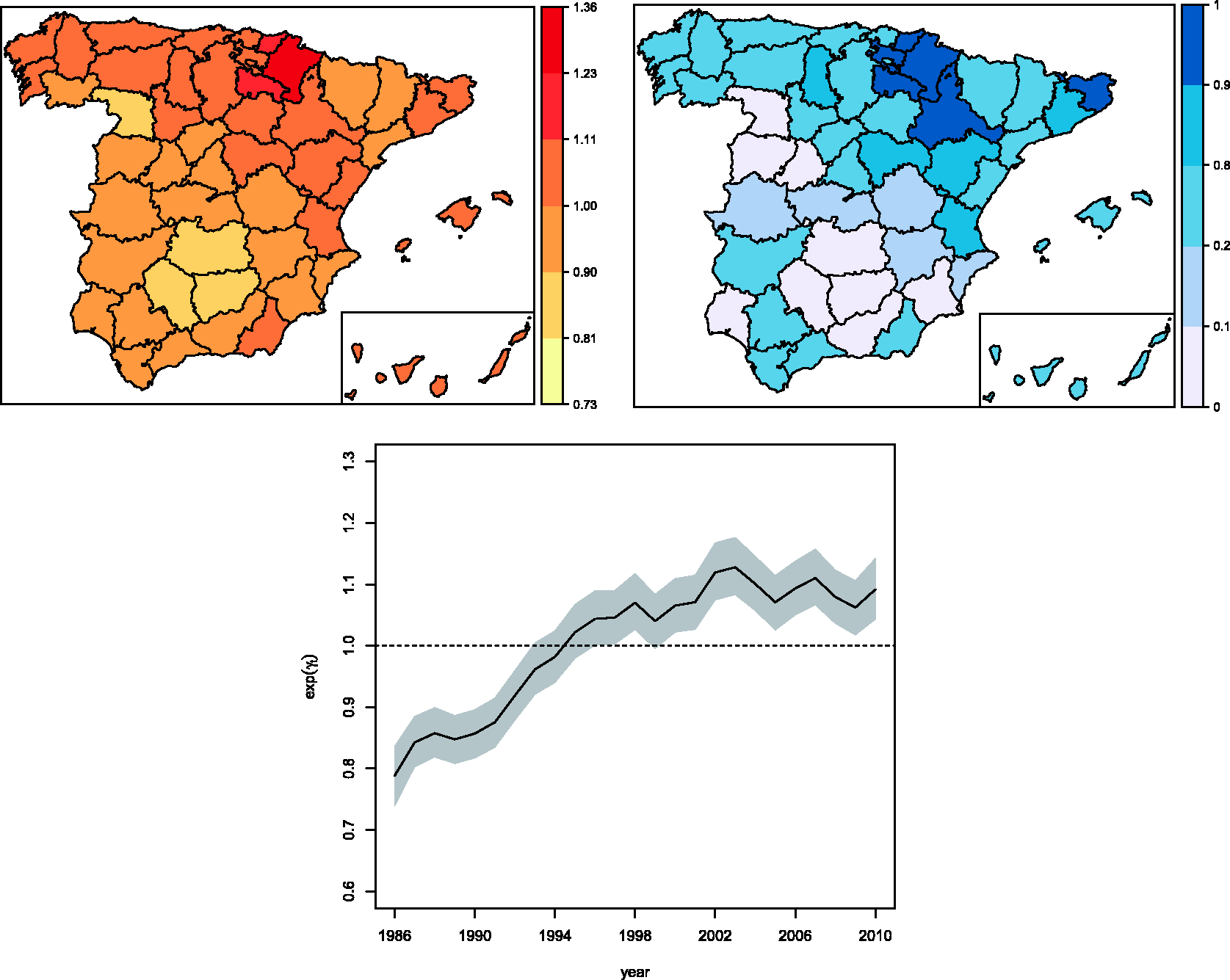

Finally, Figure 3 shows the spatio-temporal evolution of male brain cancer mortality risks for each province (comparing to the whole of Spain) in the study period (1986–2010) (top figure), and the posterior probabilities that the relative risks are greater than 1 (bottom figure). The risk scale was originally constructed in the logarithmic scale to express the same magnitudes of excess and default of risk with respect to Spain. Then, it was back-transformed to facilitate maps reading and interpretation (for example, 1.45 means 45% excess of risk with respect to Spain in the studied period and 0.69 (1/0.69) means the same amount but of risk default). Combining the information provided by both maps, an increase in risk is observed as the maps are getting darker with years. A group of provinces in the north and central-east of Spain exhibit high significant risk.

Figure 3.

Relative mortality risk distribution (top) and $P ({\overset{\land}{r}}_{it} > 1 | O)$ posterior probability distribution (bottom) by province for males.

4.1 Sensitivity analysis of hyperprior distributions

In this section, we focus the attention on Model 17 to study sensitivity to hyperpriors distributions. Different hyperpriors are considered to assess if changes in estimates of the target parameters, in their posterior distributions, and in the relative risk estimates occur. A matter of concern is also to look into changes in fixed effects. In the example considered here, the single fixed effect is the intercept. However, in ecological regression, changes affecting fixed effects can be very important to decide whether or not a covariate explains differences in risk. Our selected model has three variance parameters, $σ_{s}^{2} = 1 / τ_{s}$ , $σ_{γ}^{2} = 1 / τ_{γ}, σ_{δ}^{2} = 1 / τ_{δ}$ , and the spatial smoothing parameter λ _s . For each of these parameters, prior distributions are changed leaving the rest of parameters with the same distributions used in the data analysis.

The choice of different hyperpriors for the logit of the spatial smoothing parameter λ _s has to be done carefully. If there is little or no information about the strength of the spatial correlation, non-informative priors have to be chosen. If logit λ _s follows a logitbeta(1,1) distribution, then λ _s follows a [0,1] uniform distribution. Hyperprior parameters can be appropriately selected to allow high or low spatial dependence. In our analysis, other priors such as logitbeta(2,2) and logitbeta(0.5, 0.5) have been also considered. While the first one will favour values close to 0.5, the second one will favour more extreme values of λ _s . Additional priors favouring higher values of λ _s , such as logitbeta(5,3) and logitbeta(5,2) have also been evaluated, but they produce results similar to logitbeta(4,2), and have been omitted.

Posterior means and standard deviations for the parameters obtained with the different hyperpriors are displayed in Table 3. Hyperpriors used in the analysis of the Spanish brain cancer data are marked with an asterisk (⋆). Marginal posterior densities are shown in Figure 4.

Figure 4.

Marginal posterior densities of the variances of random effects ( $σ_{s}^{2}, σ_{γ}^{2}, σ_{δ}^{2}$ ) and spatial smoothing parameter (λ _s ) for different hyperparameters.

Table 3.

Estimated posterior mean and standard deviation of the model parameters for different hyperpriors.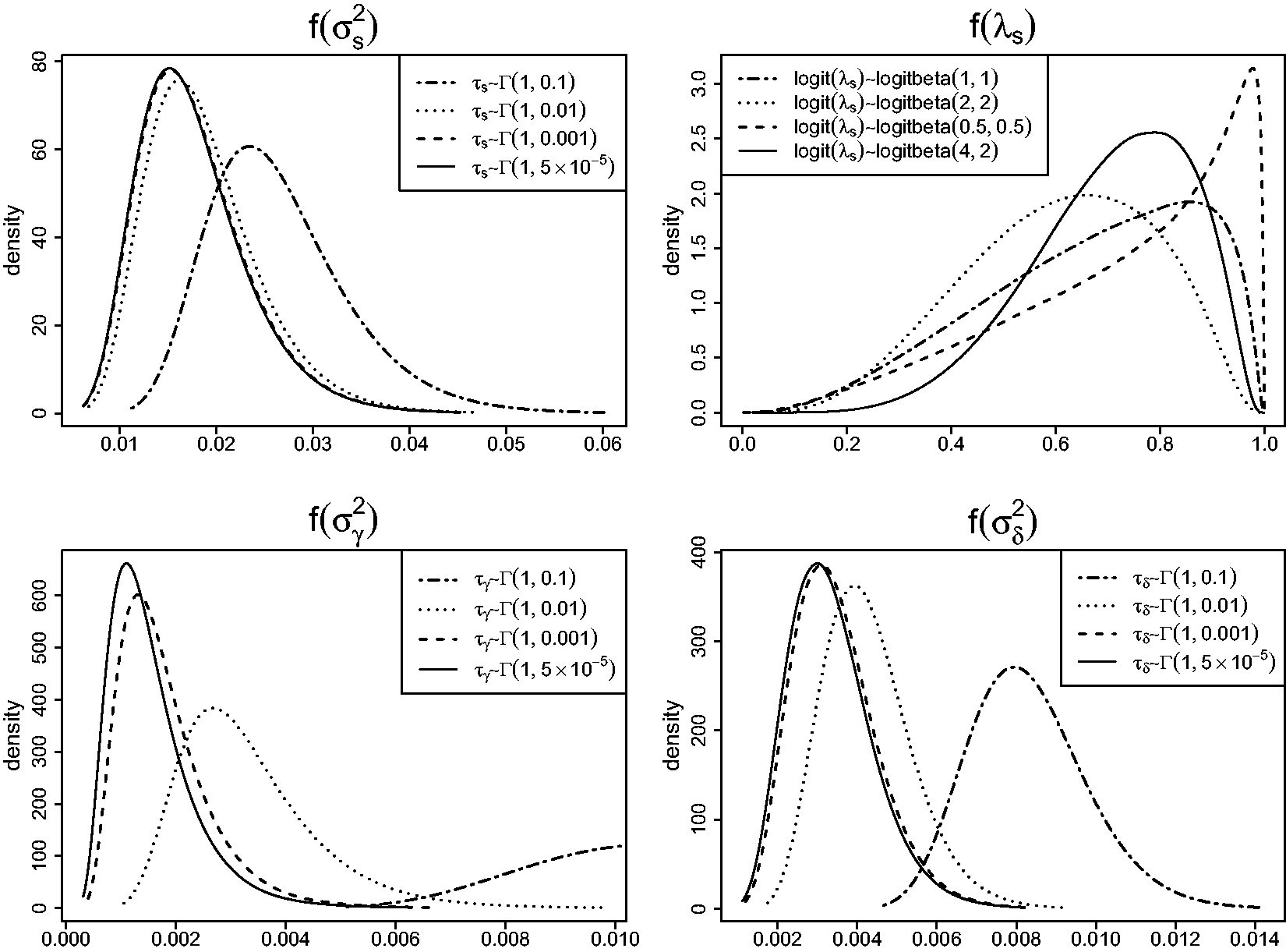

Parameter	Priors		Mean	SD	α
Parameter	Priors		Mean	SD	Mean	SD	0.025quant	0.975quant
$σ_{s}^{2}$	A1	log $τ_{s} ~$ logGamma(1, 0.1)	0.0264	0.0073	−0.023	0.054	−0.134	0.087
	A2⋆	log $τ_{s} ~$ logGamma(1, 0.01)	0.0187	0.0059	−0.022	0.043	−0.110	0.065
	A3	log $τ_{s} ~$ logGamma(1, 0.001)	0.0177	0.0058	−0.022	0.041	−0.107	0.062
	A4	log $τ_{s} ~$ logGamma $(1, 5 \times 10 - 5)$	0.0176	0.0058	−0.022	0.041	−0.106	0.062
λ _s	B1	logit $λ_{s} ~$ logitbeta(1, 1)	0.669	0.202	−0.023	0.047	−0.119	0.074
	B2	logit $λ_{s} ~$ logitbeta(2, 2)	0.608	0.177	−0.023	0.036	−0.096	0.051
	B3	logit $λ_{s} ~$ logitbeta(0.5, 0.5)	0.728	0.214	−0.022	0.070	−0.168	0.123
	B4⋆	logit $λ_{s} ~$ logitbeta(4, 2)	0.707	0.149	−0.022	0.043	−0.110	0.065
$σ_{γ}^{2}$	C1	log $τ_{γ} ~$ logGamma(1, 0.1)	0.0125	0.0038	−0.023	0.043	−0.111	0.064
	C2	log $τ_{γ} ~$ logGamma(1, 0.01)	0.0033	0.0013	−0.023	0.043	−0.110	0.064
	C3	log $τ_{γ} ~$ logGamma(1, 0.001)	0.0018	0.0009	−0.022	0.043	−0.110	0.065
	C4⋆	log $τ_{γ} ~$ logGamma $(1, 5 \times 10 - 5)$	0.0016	0.0008	−0.022	0.043	−0.110	0.065
$σ_{δ}^{2}$	D1	log $τ_{δ} ~$ logGamma(1, 0.1)	0.0083	0.0015	−0.024	0.043	−0.112	0.063
	D2	log $τ_{δ} ~$ logGamma(1, 0.01)	0.0043	0.0011	−0.023	0.043	−0.110	0.064
	D3	log $τ_{δ} ~$ logGamma(1, 0.001)	0.0035	0.0011	−0.022	0.043	−0.110	0.065
	D4⋆	log $τ_{δ} ~$ logGamma $(1, 5 \times 10 - 5)$	0.0034	0.0011	−0.022	0.043	−0.110	0.065

Note: 95% credibility intervals are shown for the fixed effect.

The marginal posterior densities and posterior mean estimates of the spatial variance $σ_{s}^{2}$ are quite similar for prior distributions A2, A3 and A4. Only the prior with the biggest inverse-scale parameter for the Gamma distribution (A1) shows significant differences with the others. The marginal posterior density of the spatial smoothing parameter λ _s exhibits certain degree of sensitivity to the hyperprior distribution. Besides some differences in the posterior means and standard errors, the posterior distribution of the fixed effect is somehow affected. In particular, differences are obtained in standard errors and credibility intervals. The prior distribution B3 leads to a wider confidence interval. This sensitivity could be important in ecological regression where one of the targets is to assess the effects of some covariates on the response. The variance parameter $σ_{γ}^{2}$ of the temporal random effect shows some sensitivity to the hyperprior choice. In Figure 4, it can be observed how the C1 and C2 hyperpriors produce very different posterior densities compared with C3 and C4 priors. Schrödle and Held²⁷ show that if the random effect γ is modelled as a RW2, the prior for $τ_{γ}$ has to be chosen with care as the results can be sensitive to that choice. In our example, this issue should also be taken into account when γ is modelled as a RW1. Similar conclusions can be obtained for the variance parameter of the spatio-temporal random effect $σ_{δ}^{2}$ .

Robustness of the posterior relative risks distribution to hyperprior choice has been also studied. Figure 5 displays absolute errors between estimated relative risks for different hyperpriors. For each model parameter, the hyperprior used in the analysis of brain cancer mortality has been compared with the others. The maximum absolute difference for the estimated risks relative to τ _s hyperpriors A2, A3 and A4 is around $5 e - 3$ . The maximum absolute difference with regard to hyperpriors for τ_γ and τ_δ is about $1 e - 1$ and $5 e - 2$ , respectively. These quantities do not mean any important difference in risks.

Figure 5.

Boxplots of the absolute errors between estimated relative risk for different prior distributions.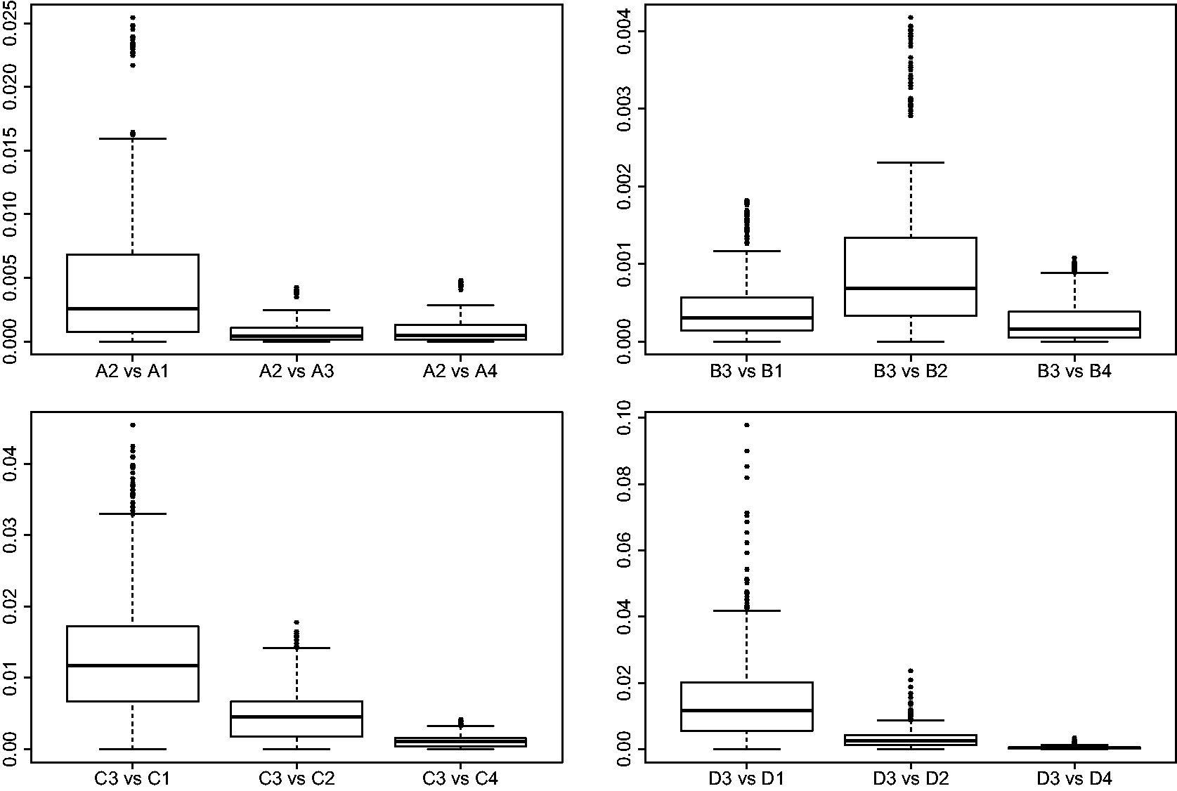

4.2 Comparing likelihood-based inference and INLA

Spatio-temporal disease mapping models are GLMM’s, and likelihood-based inference can be performed relatively easy using PQL. There has been some research comparing PQL and MCMC methods,^45,46 and MCMC and INLA,^29,4 but little research has been conducted comparing INLA and PQL in disease mapping. Fong et al.⁷ compare PQL and INLA analysing specific data set under GLMMs. In particular, in the supplementary material of their paper, they revisit the widely used Scotish lip cancer data with INLA and PQL obtaining similar estimates and standard errors. In this section, a comparison of INLA and PQL based on the analysis of the Spanish brain cancer data is provided. Parameter estimates and standard errors obtained with both methods are displayed in Table 4. INLA and PQL estimates for the model parameters are, in general, quite similar. The largest discrepancy is obtained for the spatial smoothing parameter λ _s , where the estimated standard errors with PQL is larger than the one derived from INLA. With regard to risk estimates, differences between the two methods are very small. The maximum absolute error between INLA and PQL is about $1 e - 2$ . Figure 6 displays a dispersion plot of PQL vs. INLA relative risk estimates. All points are in the main diagonal indicating an almost perfect match between both methods.

Figure 6.

PQL vs. INLA relative risk estimates.

Table 4.

Model parameter estimates and standard errors obtained by PQL and INLA.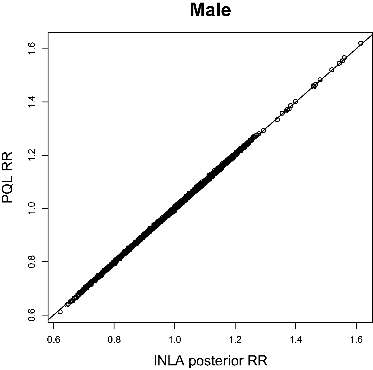

	Male
	PQL	INLA
α	−0.020 (0.055)	−0.022 (0.043)
$σ_{s}^{2}$	0.020 (0.007)	0.019 (0.006)
λ _s	0.865 (0.339)	0.707 (0.149)
$σ_{γ}^{2}$	0.0017 (0.0008)	0.0016 (0.0008)
$σ_{δ}^{2}$	0.0035 (0.0010)	0.0034 (0.0011)

5 Simulation study

In this section, a simulation study is conducted to compare INLA and PQL more formally in the spatio-temporal setting of the Spanish male brain cancer mortality data considered in this paper. Here, 500 data sets have been generated according to the next procedure. For each data set

k = 1, \dots, 500

, the random effects are generated from the following multivariate normal distributions

ξ ~ N (0, {\overset{\land}{σ}}_{s}^{2} (\overset{\land}{} λ_{s} R_{s} + (1 - (\overset{\land}{} λ_{s}) I_{s}) - 1) γ ~ N (0, {\overset{\land}{σ}}_{γ}^{2} R_{t}^{-}) δ ~ N (0, {\overset{\land}{σ}}_{δ}^{2} (R_{t} \otimes R_{s}) -)

where

{\overset{\land}{σ}}_{s}^{2}, {\overset{\land}{λ}}_{s}, {\overset{\land}{σ}}_{γ}^{2}

and

{\overset{\land}{σ}}_{δ}

are approximately the average of the PQL and INLA estimates given in Table 4. Then, the simulated log-relative risks are

b_{it}^{k} = \log r_{it}^{k} = \overset{\land}{α} + ξ_{i}^{k} + γ_{t}^{k} + δ_{it}^{k}

and the counts are generated from a Poisson distribution with mean

μ_{it} = E_{it} exp (b_{it}^{k})

. To study the effect of the population, this escenario has also been repeated multiplying the expected counts by the scale factors 0.5, 2 and 4. For each simulation, a Type IV space-time interaction model (Model 17) has been fitted using INLA and PQL. For the INLA approach, the same set of hyperpriors used in the data analysis has been considered in the simulation study. That is,

\log τ_{s} ~ logGamma (1, 0.01), logit λ_{s} ~ logitbeta (4, 2), \log τ_{γ} ~ logGamma (1, 5 \times 10 - 5)

and

\log τ_{δ} ~ logGamma (1, 5 \times 10 - 5)

. Table 5 displays the mean values of INLA and PQL estimated parameters over the 500 data sets. In general, mean values of estimated parameters with INLA for the 500 simulated data are more similar to the true values, except for the temporal variance component

σ_{γ}^{2}

where PQL provides a better result. Note that both methods provide approximately unbiased estimates irrespective of the population size.

Table 5.

Mean values of INLA and PQL estimated parameters based on 500 simulated data sets for scenario 4.

Parameter	True value	INLA Estimate				PQL Estimate
Parameter	True value	SF = 0.5	SF = 1	SF = 2	SF = 4	SF = 0.5	SF = 1	SF = 2	SF = 4
α	−0.0215	−0.0237	−0.0221	−0.0199	−0.0226	−0.0208	−0.0199	−0.0182	−0.0214
$σ_{s}^{2}$	0.0190	0.0185	0.0179	0.0181	0.0185	0.0172	0.0167	0.0168	0.0173
λ _s	0.7500	0.6720	0.6720	0.6670	0.6680	0.6450	0.6610	0.6470	0.6570
$σ_{γ}^{2}$	0.0025	0.0020	0.0022	0.0024	0.0025	0.0024	0.0024	0.0026	0.0026
$σ_{δ}^{2}$	0.0035	0.0033	0.0035	0.0034	0.0034	0.0035	0.0036	0.0035	0.0035

Table 6 provides true simulated standard errors and the corresponding standard error estimates obtained with INLA and PQL. The simulated standard errors are derived from the sample variance of the 500 parameter estimates. The estimated standard errors for INLA are calculated as the square root of

\overset{\land}{Var} (\overset{\land}{θ}) = E [\overset{\land}{θ} 2] - E [\overset{\land}{θ}] 2

. The PQL standard errors are obtained asymptotically from the inverse of the Fisher information matrix (see for example Ugarte et al.¹⁹). Figures in Table 6 are multiplied by 100 to better interpret the results. Both methods overestimate the standard error for the spatial smoothing parameter λ _s . The simulated standard error reveals that PQL estimates are much more variable than INLA estimates (for SF = 1, the simulated standard error for INLA is 7.24, and for PQL is 28.21). However, INLA estimates of the standard error are twice the simulated values (15.42/7.24 = 2.13) while for PQL is around 1.25 times the simulated error (34.64/28.21 = 1.23). This actually means that INLA estimates of the standard error of the spatial smoothing parameter λ _s are worse than those provided by PQL. The standard errors of the remaining parameters are reasonably well estimated.

Table 6.

Simulated standard errors (sim) and mean values of INLA and PQL estimated parameters standard errors (est) based on 500 simulated data sets for scenario 4.

Parameter	INLA estimate × 10²
	SF = 0.5		SF = 1		SF = 2		SF = 4
	sim	est	sim	est	sim	est	sim	est
α	4.14	4.21	3.85	4.06	4.11	4.00	3.92	4.02
$σ_{s}^{2}$	0.66	0.69	0.49	0.58	0.46	0.54	0.44	0.51
λ _s	6.43	15.83	7.24	15.42	7.76	15.17	8.02	14.91
$σ_{γ}^{2}$	0.14	0.25	0.11	0.11	0.10	0.10	0.09	0.09
$σ_{δ}^{2}$	0.14	0.13	0.10	0.10	0.08	0.08	0.06	0.06
PQL estimate × 10²
α	4.14	3.39	3.84	3.60	4.11	3.35	3.92	3.48
$σ_{s}^{2}$	0.77	0.76	0.59	0.64	0.55	0.60	0.56	0.59
λ _s	31.15	39.03	28.21	34.64	26.95	32.24	26.42	30.77
$σ_{γ}^{2}$	0.14	0.14	0.10	0.11	0.09	0.10	0.08	0.09
$σ_{δ}^{2}$	0.14	0.13	0.10	0.10	0.07	0.08	0.06	0.06

Empirical coverage rates for model parameters have been also computed. Results are displayed in Table 7. The distribution of the PQL estimator of the variance components

σ_{s}^{2}, σ_{γ}^{2}

and

σ_{δ}^{2}

has not been approximated by the normal distribution as Dean et al.^9,47 report. They suggest using a Wilson-Hilferty transformation for

χ 2

random variables (see Johnson and Kotz,⁴⁸ chap. 17), and this is the approach considered here. For α and λ _s , the normal approximation has been used. However, estimates of the α parameter are rather variable in our simulation study and that is the reason for the poor coverage rates. The more extreme values of this parameter correspond to extreme estimates of the smoothing parameter λ _s . If we remove these extreme values, a significant improvement in coverage rates is achieved. Coverage rates for λ _s obtained with INLA credibility intervals lead to a clear over-coverage. This is not surprising as INLA overestimates the standard error. Nevertheless, care is recommended with estimates of the spatial smoothing parameter as they are rather variable and unstable. Finally, coverage rates for the spatial variance components seem to be slightly better with INLA, while PQL provides better coverage rates for the temporal component. Regarding the interaction term, both methods lead to similar results.

Table 7.

Empirical coverage probabilities of the estimated parameters in both PQL and INLA estimation methods.

Parameter	PQL			INLA
Parameter	90%	95%	99%	90%	95%	99%
α	68.0	73.4	80.2	88.6	96.0	99.6
$σ_{s}^{2}$	95.2	97.2	98.0	91.4	96.2	99.2
λ _s	86.4	90.1	95.1	100	100	100
$σ_{γ}^{2}$	95.6	97.4	99.6	80.4	86.8	95.2
$σ_{δ}^{2}$	91.2	94.6	97.2	88.2	94.4	98.8

The accuracy and precision of INLA and PQL to estimate relative risks has been evaluated computing the Mean Absolute Relative Bias (MARB) and the Mean Relative Root Mean Prediction Error (MRRMPSE) for each province. These measures are calculated averaging over the areas the following quantities

{MARB}_{i} = \frac{1}{T} \sum_{t = 1}^{T} \frac{1}{500} | \sum_{k = 1}^{500} \frac{{\overset{\land}{r}}_{it}^{k} - r_{it}^{k}}{r_{it}^{k}} |, {MRRMPSE}_{i} = \frac{1}{T} \sum_{t = 1}^{T} \sqrt{\frac{1}{500} \sum_{k = 1}^{500} (\frac{{\overset{\land}{r}}_{it}^{k} - r_{it}^{k}}{r_{it}^{k}}) 2} .

Results are displayed in Table 8. While relative errors are almost similar, the bias for the estimated risks with PQL is slightly smaller than those obtained with INLA.

Table 8.

Average values of mean absolute relative bias (MARB) and mean relative root mean prediction error (MRRMPSE) of the relative risks estimated by INLA and PQL based on 500 simulated data sets for scenario 4.

	INLA Estimate				PQL Estimate
	SF = 0.5	SF = 1	SF = 2	SF = 4	SF = 0.5	SF = 1	SF = 2	SF = 4
MARB	0.0078	0.0065	0.0047	0.0031	0.0065	0.0056	0.0040	0.0027
MRRMPSE	0.0858	0.0732	0.0613	0.0501	0.0853	0.0737	0.0612	0.0500

In summary, differences between PQL and INLA to estimate relative risks become moot. Both approaches perform well when estimating variance components too. However, there are some differences regarding the estimation of the spatial smoothing parameter λ _s . Although both methods provide reasonably good point estimates (bias is slightly smaller for INLA), estimates are rather variable. A simulation study has been also conducted using a non-informative prior $logit (λ_{s}) ~ logitbeta (1, 1)$ for the spatial variability parameter λ _s . Results are rather similar (not shown here), but the INLA estimates for λ _s increase their variability substantially, being the simulated standard error now twice the simulated standard error obtained when using the informative prior $logit (λ_{s}) ~ logitbeta (4, 2)$ .

6 Discussion

INLA emerges as a powerful tool for Bayesian inference overcoming some inconveniences of MCMC algorithms. In particular, the technique is based on a series of Laplace approximations reducing computing time substantially while attaining a high degree of accuracy. The possibility of fitting models with INLA in a widespread software, such as R, is a reality, thanks to the package R-INLA. This contributes to a general use and knowledge of the technique. The computational speed of the INLA methodology allows to fit many models easily, something simply unfeasible if complex models have to be fitted using computationally expensive MCMC algorithms. Consequently, sensitivity analyses, which requires fitting the model with different prior distributions, could be routinely carried out. The INLA methodology also provides the deviance information criterion (DIC), a well-known Bayesian model selection criterion to choose the best model among different candidates.

Most of the research into spatio-temporal disease mapping with INLA is based on the well-known BYM convolution model with an iCAR prior for the spatial random effects. However, this prior has been shown to produce negative correlations between far apart areas,^31,32 and the Leroux CAR prior, a less widely used prior in disease mapping, is considered instead. This model is not a ready to use option in INLA yet (at least at the time of writing this paper), but it can be easily implemented as shown in this paper. A comparison of INLA and PQL has been conducted using the Leroux CAR prior for the spatial random effects. PQL has been used for a long time in EB disease mapping and it is still working very well when fitting mixed Poisson models in space–time disease mapping and data dimension is not too big. Our simulation study evaluates the performance of INLA and PQL and reveals some interesting results. Both procedures provide similar parameter estimates. Mean values of standard errors are also rather similar except for the smoothing parameter, where INLA tends to overestimate the standard error a bit more than PQL. This parameter is rather unstable and caution is always recommended. The PQL estimator of the α-parameter also deserves attention. In our simulation study, estimates are rather variable and extreme values match up with extreme values of λ _s . Nevertheless, both methods provide nearly identical estimates for the relative risks, and INLA estimates of these quantities are robust to the choice of hyperpriors. However, it should be stated that even though the posterior estimates of the relative risks are not affected, the posterior distributions of the precision parameters can be very sensitive to hyperprior distributions as it has been shown in this paper. A matter of possible concern is the sensitivity of the fixed effects to the hyperprior selection. In particular, different distributions for the spatial smoothing parameter λ _s could lead to some changes on the credibility intervals for the fixed effects. This could be important in ecological regression where the target is to assess the effects of some covariates on the response.

Finally, our analysis of the Spanish male brain cancer mortality data in the period 1986–2010 reveals that mortality is still high, and provinces located in the north show a significant high risk in comparison with the whole country. In particular, Navarre and the Basque provinces exhibit the highest risks. The reasons why these regions show high brain cancer mortality risks still remain unknown and further research is needed.

Footnotes

Funding

This research has been supported by the Spanish Ministry of Science and Innovation (MTM 2011-22664 which is co-funded by FEDER grants).

Acknowledgments

The authors would like to thank the National Epidemiology Center (area of Environmental Epidemiology and Cancer) for providing the data and for fruitful discussion on the data analysis. Thanks are also given to a reviewer for his/her useful comments that have contributed to the improvement of the paper.

Appendix

References

Goicoa

Ugarte

Etxeberría

. Comparing CAR and P-spline models in spatial disease mapping. Environ Ecol Stat 2012; 19: 573–599.

Spiegelhalter DJ, Thomas A, Best NG, et al. WinBUGS version 1.4 user’s manual. MRC Biostatiscs unit. Cambridge: Institute of Public Health; Rolf Nevanlinna Institute, University of Helsinki; and Department of Epidemiology and Public Health, Imperial College London, http://www.mrc-bsu.cam.ac.uk/bugs/winbugs/manual14.pdf (accessed on 28 February 2014).

Lawson AB. Bayesian disease mapping: Hierarchal modeling in spatial epidemiology. 2nd ed. Boca Raton: Chapman & Hall/CRC Interdisciplinary Statistics, 2013.

Schrödle

Held

Riebler

. Using integrated nested Laplace approximations for the evaluation of veterinary surveillance data from Switzerland: a case-study. J Roy Stat Soc C 2011; 60: 261–279.

Schmid

Held

. Bayesian extrapolation of space-time trends in cancer registry data. Biometrics 2004; 60: 1034–1042.

Wakefield

. Disease mapping and spatial regression with count data. Biostatistics 2007; 8: 158–183.

Fong

Rue

Wakefield

. Bayesian inference for generalized linear mixed models. Biostatistics 2010; 11: 397–412.

Breslow

Clayton

. Approximate inference in generalized linear mixed models. J Am Stat Assoc 1993; 88: 9–25.

Dean

Ugarte

Militino

. Penalized quasi-likelihood with spatially correlated data. Comput Stat Data Anal 2004; 45: 235–248.

10.

Breslow NE. Whither PQL? In: Lin D and Heagerty PJ (eds) Proceedings of the second Seattle symposium. New York: Springer, 1993, pp.1–22.

11.

Ugarte

Militino

Goicoa

. Prediction error estimators in Empirical Bayes disease mapping. Environmetrics 2008; 19: 287–300.

12.

Bernardinelli

Clayton

Pascutto

. Bayesian analysis of space-time variation in disease risk. Stat Med 1995; 14: 2433–2443.

13.

Assunção

Reis

Oliveira

. Diffusion and prediction of leishmaniasis in a large metropolitan area in Brazil with a Bayesian space-time model. Stat Med 2001; 20: 2319–2335.

14.

Knorr-Held

. Bayesian modelling of inseparable space-time variation in disease risk. Stat Med 2000; 19: 2555–2567.

15.

Martínez-Beneito

López-Quílez

Botella-Rocamora

. An autoregressive approach to spatio-temporal disease mapping. Stat Med 2008; 27: 2874–2889.

16.

Ugarte

Goicoa

Ibáñez

. Evaluating the performance of spatio-temporal Bayesian models in disease mapping. Environmetrics 2009; 20: 647–665.

17.

Besag

York

Mollié

. Bayesian image restoration, with two applications in spatial statistics. An I Stat Math 1991; 43: 1–20.

18.

MacNab

Dean

. Autoregressive spatial smoothing and temporal spline smoothing for mapping rates. Biometrics 2001; 57: 949–956.

19.

Ugarte

Goicoa

Militino

. Spatio-temporal modeling of mortality risks using penalized splines. Environmetrics 2010; 21: 270–289.

20.

Ugarte

Goicoa

Etxeberría

. Projections of cancer mortality risks using spatio-temporal P-spline models. Stat Methods Med Res 2012; 21: 545–560.

21.

Ugarte

Goicoa

Etxeberría

. A P-spline ANOVA type model in space-time disease mapping. Stoch Env Res Risk A 2012; 26: 835–845.

22.

MacNab

. Spline smoothing in Bayesian disease mapping. Environmetrics 2007; 18: 727–744.

23.

MacNab

Gustafson

. Regression B-spline smoothing in Bayesian disease mapping: with an application to patient safety surveillance. Stat Med 2007; 26: 4455–4474.

24.

Rue

Martino

Chopin

. Approximate Bayesian inference for latent Gaussian models by using integrated nested Laplace approximations. J Roy Stat Soc B 2009; 71: 319–392.

25.

R Core Team. R: A language and environment for statistical computing. R Foundation for Statistical Computing. Vienna, Austria, http://www.R-project.org/ (2013, accessed on 28 February 2014).

26.

Martino S and Rue H. Implementing approximate Bayesian inference using integrated nested Laplace approximation: A manual for the inla program. Department of Mathematical Sciences, NTNU, Norway, http://www.math.ntnu.no/ hrue/GMRFLib (2009).

27.

Schrödle

Held

. A primer on disease mapping and ecological regression using INLA. Computation Stat 2011; 26: 241–258.

28.

Schrödle

Held

. Spatio-temporal disease mapping using INLA. Environmetrics 2011; 22: 725–734.

29.

Held

Schrödle

Rue

Posterior and cross-validatory predictive checks: A comparison of MCMC and INLA. In: Kneib

Tutz

(eds). Statistical modelling and regression structures, Heidelberg: Physica, 2010, pp. 91–110.

30.

Blangiardo

Cameletti

Baio

. Spatial and spatio-temporal models with R-INLA. Spat Spatiotemporal Epidemiol 2013; 4: 33–49.

31.

MacNab

. On Gaussian Markov random fields and Bayesian disease mapping. Stat Methods Med Res 2011; 20: 49–68.

32.

Botella-Rocamora

López-Quílez

Martínez-Beneito

. Spatial Moving Average Risk Smoothing. Stat Med 2013; 32: 2595–2612.

33.

MacNab YC. On identification in Bayesian disease mapping and ecological-spatial regression models. Stat Methods Med Res. DOI: 10.1177/0962280212447152. Available at: http://smm.sagepub.com/search/results?fulltext=MacNab&x=11&y=14&submit=yes&journal_set=spsmm&src=selected&andorexactfulltext=and.

34.

Leroux

Lei

Breslow

Estimation of disease rates in small areas: A new mixed model for spatial dependence. In: Halloran

Berry

(eds). Statistical models in epidemiology, the environment and clinical trials, New York: Springer-Verlag, 1999, pp. 135–178.

35.

Lee

. A comparison of conditional autoregressive models used in bayesian disease mapping. Spat Spatiotemporal Epidemiol 2011; 2: 79–89.

36.

Lee

Mitchell

. Locally adaptive spatial smoothing using conditional autoregressive models. J Roy Stat Soc C 2013; 62: 593–608.

37.

Rue

Held

. Gaussian Markov random fields: theory and applications, Boca Raton, FL: Chapman & Hall/CRC, 2005.

38.

Clayton

Generalized linear mixed models. In: Gilks

(eds). Markov Chain Monte Carlo in practice, London: Chapman and Hall, 1996.

39.

Tierney

Kadane

. Accurate approximations for posterior moments and marginal densities. J Am Stat Assoc 1986; 81: 82–86.

40.

Martins

Simpson

Lindgren

. Bayesian computing with INLA: new features. Comput Stat Data Anal 2013; 67: 68–83.

41.

Rue

Martino

. Approximate Bayesian inference for hierarchical Gaussian Markov random field models. J Stat Plan Infer 2007; 137: 3177–3192.

42.

Spiegelhalter

Best

Carlin

. Bayesian measures of model complexity and fit. J Roy Stat Soc B 2002; 64: 583–639.

43.

López-Abente

Pollán

Ardanaz

. Geographical pattern of brain cancer incidence in the Navarre and Basque Country regions of Spain. Occup Environ Med 2003; 60: 504–508.

44.

Richardson

Thomson

Best

. Interpreting posterior relative risk estimates in disease-mapping studies. Environ Health Pesp 2004; 112: 1016–1025.

45.

Ugarte

Goicoa

Militino

. Empirical Bayes and Fully Bayes procedures to detect high risk areas in disease mapping. Comput Stat Data Anal 2009; 53: 2938–2949.

46.

Ainsworth

Dean

. Approximate inference for disease mapping. Comput Stat Data Anal 2006; 50: 2552–2570.

47.

Dean

Ugarte

Militino

. Detecting interaction between random region and fixed age effects in disease mapping. Biometrics 2001; 57: 197–202.

48.

Johnson

Kotz

. Distributions in statistics: continuous univariate distributions 1970; Vols 1 and 2, New York: Wiley.

49.

Seneta

. Non-negative matrices and Markov Chains, New York: Springer-Verlag, 1981.

50.

Rao CR and Rao MB. Matrix algebra and its applications to statistics and econometrics. Singapore: World Scientific Publishing Company, 1998.

Supplementary Material

Please find the following supplemental material available below.

For Open Access articles published under a Creative Commons License, all supplemental material carries the same license as the article it is associated with.

For non-Open Access articles published, all supplemental material carries a non-exclusive license, and permission requests for re-use of supplemental material or any part of supplemental material shall be sent directly to the copyright owner as specified in the copyright notice associated with the article.

0.00 MB

0.13 MB

0.12 MB