Sample size calculation for treatment effects in randomized trials with fixed cluster sizes and heterogeneous intraclass correlations and variances

Abstract

When comparing two different kinds of group therapy or two individual treatments where patients within each arm are nested within care providers, clustering of observations may occur in both arms. The arms may differ in terms of (a) the intraclass correlation, (b) the outcome variance, (c) the cluster size, and (d) the number of clusters, and there may be some ideal group size or ideal caseload in case of care providers, fixing the cluster size. For this case, optimal cluster numbers are derived for a linear mixed model analysis of the treatment effect under cost constraints as well as under power constraints. To account for uncertain prior knowledge on relevant model parameters, also maximin sample sizes are given. Formulas for sample size calculation are derived, based on the standard normal as the asymptotic distribution of the test statistic. For small sample sizes, an extensive numerical evaluation shows that in a two-tailed test employing restricted maximum likelihood estimation, a safe correction for both 80% and 90% power, is to add three clusters to each arm for a 5% type I error rate and four clusters to each arm for a 1% type I error rate.

Keywords

Individually randomized group treatment maximin design optimal design sample size therapist effects

1 Introduction

Many study designs evaluating the effect of an intervention are characterized by observations being correlated within clusters. This may arise in group or cluster randomized trials,¹ where groups are the units of assignment. In such trials, groups are assigned to one of several treatment conditions and all sampled members of the same group are given the same treatment. For example, school classes with all of its pupils are assigned to a smoking prevention program, or general practices with all of its sampled patients are assigned to one of several medication regimens. However, when individuals, instead of groups, are the units of assignment, clustering of observations may also occur. This is the case when the treatment itself induces clustering, such as when treatments are given to groups of individuals.^2,3 In such individually randomized group treatment trials, interactions between persons within a group may lead to the observations on the outcome variable being correlated.⁴ The clustering may occur in only one of the treatment arms, such as when group therapy is compared to a treatment condition involving only medication,^5,6 but also in both treatment arms, when, for instance, two different types of group therapy are compared.^7,8 Clustering effects due to treatment may also occur if the treatment is not given to a group as a whole but on an individual basis. If several patients are treated by the same therapist or, more generally, the same care provider, then patients of one therapist will be treated in a more similar way than patients treated by different therapists. Such therapist effects may also lead to correlated observations within clusters.^3,4,9

The present paper will address sample size calculation for trials comparing group administered interventions or trials where clustering effects are due to therapists, assuming a quantitative outcome variable and estimation of the treatment effect by maximum likelihood (ML) in a linear mixed model analysis. For the case of homogeneity between the treatment arms with respect to outcome variance, intraclass correlation, cluster size, and number of clusters, formulas for sample size calculation have been derived by Raudenbush¹, Moerbeek et al.,¹⁰ and Liu.¹¹ The present study generalizes these results by considering treatment arms that differ in outcome variance, intraclass correlation, cluster size, and number of clusters, for a scenario where the cluster sizes are more or less fixed. This would apply when therapy groups have some ideal group size that is rather fixed, or when therapists have some ideal caseload.

The paper is structured as follows. Section 2 presents the linear mixed effects model for trials comparing two arms, allowing for a difference between both arms with respect to the intraclass correlation, the outcome variance, the number of clusters, and the cluster size. Section 3 gives an explicit expression for the asymptotic variance of the treatment effect estimator and presents the optimal number of clusters for each treatment arm, optimal meaning that these numbers minimize the variance of the treatment effect estimator and thus maximize the test power under cost constraints. Section 4 gives formulas to calculate the optimal number of clusters needed for a given effect size (ES) and power level (as opposed to a given budget) and presents some analytical results for these optimal sample sizes. To handle uncertainty about those model parameters on which the optimal sample size depends, section 5 presents the maximin design as a robust alternative to the optimal design. Section 6 is a numerical evaluation of corrections in sample size calculation for finite samples when starting from the normal distribution as the asymptotic distribution of the test statistic. Section 7 illustrates how to apply the results in sample size calculation and section 8 summarizes the present study’s implications for planning trials.

2 Specification of the linear mixed effects model

In the treatment and control condition, we have respectively K_t and K_c clusters (such as K_t and K_c therapy groups). In each cluster j (j = 1,…, K_t) of the treatment condition, there are m persons and in each cluster j (j = K_t + 1,…, K_t + K_c) of the control condition, there are n persons, the total number of persons thus amounting to N = K_tm + K_cn. The dependent variable is a quantitative outcome, denoted as y_ij for person i in cluster j (j = 1,…, K_t + K_c). If in each condition, y_ij is (approximately) normally distributed, the following linear mixed effects model is an adequate tool for data analysis^3,9

y_{ij} = β_{0} + (β_{1} + u_{j} + δ_{ij}) {Int}_{ij} + (v_{j} + ɛ_{ij}) (1 - {Int}_{ij})

(1)

where Int_i_j denotes the treatment condition for person i in cluster j, which is coded as 1 for persons in the treatment condition and coded 0 for persons in the control condition. With this coding scheme,

β_{0}

represents the mean outcome of the control condition and

β_{1}

represents the treatment effect, such as the mean outcome difference between cognitive behavioral therapy and psychodynamic interpersonal psychotherapy.⁸ Commonly,

β_{1}

is the parameter of primary interest. The terms u_j and v_j represent the random cluster effect in the treatment and control condition, respectively, whereas

δ_{ij}

and

ɛ_{ij}

represent a random person effect in these conditions. The effects u_j, v_j,

δ_{ij}

, and

ɛ_{ij}

are assumed to be independently normally distributed with respective variances

σ_{u}^{2}

σ_{v}^{2}

σ_{δ}^{2}

, and

σ_{ɛ}^{2}

. The total outcome variances for the treatment and control arm are thus

σ_{y_{t}}^{2} = σ_{u}^{2} + σ_{δ}^{2}

and

σ_{y_{c}}^{2} = σ_{v}^{2} + σ_{ɛ}^{2}

In what follows the intraclass correlation, which measures the dependency among observations for members within the same cluster, is relevant. For the model in equation (1), the intraclass correlations are $ρ_{t} = σ_{u}^{2} / (σ_{u}^{2} + σ_{δ}^{2}) = σ_{u}^{2} / σ_{y_{t}}^{2}$ for the treatment arm and $ρ_{c} = σ_{v}^{2} / (σ_{v}^{2} + σ_{ɛ}^{2}) = σ_{v}^{2} / σ_{y_{c}}^{2}$ for the control arm. The correlation between two randomly drawn persons from two different clusters, possibly from two different treatment arms, is zero.

3 Optimal number of clusters for the treatment effect under a cost constraint

Let ξ = (m,n,K_t,K_c) denote the design of a randomized trial with clustering in both arms, and let $var ({\overset{\land}{β}}_{1} | ξ)$ be the asymptotic variance of the estimator of treatment effect $β_{1}$ , given this design ξ. As can be derived from equation (14) in Appendix A, the asymptotic variance of the maximum likelihood estimator (and of the restricted maximum likelihood (REML) estimator, see Demidenko¹²) of the treatment effect, ${\overset{\land}{β}}_{1}$ , is given by

var ({\overset{\land}{β}}_{1} | ξ) = ((m - 1) ρ_{t} + 1) (\frac{σ_{y_{t}}^{2}}{m K_{t}}) + ((n - 1) ρ_{c} + 1) (\frac{σ_{y_{c}}^{2}}{n K_{c}})

(2)

This variance increases as a function of the intraclass correlations $ρ_{t}$ and $ρ_{c}$ and the variances within the treatment arms $σ_{y_{t}}^{2}$ and $σ_{y_{c}}^{2}$ , and decreases as a function of the cluster sizes m and n and the number of clusters K_t and K_c. Note that the variance of the treatment effect estimator in equation (2) is equal to the sum of the variances of the outcome mean estimator in the treatment condition and of the outcome mean estimator in the control condition. Furthermore, the factors $(m - 1) ρ_{t} + 1$ and $(n - 1) ρ_{c} + 1$ are design effects reflecting how much larger these variances are compared to variances for data where there is no clustering.

We derive a design, that is, ξ = (m,n,K_t,K_c), that minimizes the variance of the treatment estimator in equation (2) and thus maximizes test power for a fixed budget. We call this the optimal design. Finding optimal designs requires a cost function specifying the relation between the total budget required and the costs per subject/person/patient/individual and per cluster/group in a trial. Let C₀ be the overhead costs of the trial, that is, all costs which do not depend on the sample size. Let c_t and s_t be the costs per cluster and per subject in the treatment arm respectively, and let c_c and s_c be the cost per cluster and per subject in the control arm. The total study cost C then equals

C = C_{0} + K_{t} (c_{t} + m s_{t}) + K_{c} (c_{c} + n s_{c})

(3)

This cost function can be used as constraint on the total study cost when maximizing the power and precision for the treatment effect, or to minimize the total study cost while keeping power and precision constant. As a special case of the latter aim, if one is interested in minimizing the total number of subjects sampled, that is, K_tm + K_cn, let s_t = s_c = 1 and c_t = c_c = 0. Further, for individually randomized group treatment trials, there often is an ideal group size, or, for cluster randomized trials, there may be practical limitations leading to a fixed group size for each of the treatments (e.g. a school class with all of its pupils participating in a prevention trial). In such cases, we may consider m and n fixed and can rewrite equation (3) as

C = C_{0} + K_{t} c_{t}^{*} + K_{c} c_{c}^{*}

(4)

where

c_{t}^{*} = c_{t} + m s_{t}

and

c_{c}^{*} = c_{c} + n s_{c}

are the total costs of a treatment and control cluster. Starting from a fixed budget and fixed cluster/group size for each of the treatment arms, it can be proven (see Appendix A) that the following cluster numbers minimize the variance of the treatment estimator in equation (2)

K_{t}^{opt} = \frac{(C - C_{0})}{\sqrt{{c_{c}^{*} c}_{t}^{*}} (\sqrt{(\frac{σ_{y_{c}}^{2}}{σ_{y_{t}}^{2}}) (\frac{m}{n}) (\frac{(n - 1) ρ_{c} + 1}{(m - 1) ρ_{t} + 1})}) + c_{t}^{*}}, and K_{c}^{opt} = \frac{(C - C_{0})}{\sqrt{{c_{c}^{*} c}_{t}^{*}} (\sqrt{(\frac{σ_{y_{t}}^{2}}{σ_{y_{c}}^{2}}) (\frac{n}{m}) (\frac{(m - 1) ρ_{t} + 1}{(n - 1) ρ_{c} + 1})}) + c_{c}^{*}}

(5)

from which it follows, after some rewriting, that the ratio of optimal cluster numbers is equal to

\frac{K_{t}^{opt}}{K_{c}^{opt}} = \sqrt{(\frac{σ_{y_{t}}^{2}}{σ_{y_{c}}^{2}}) (\frac{n}{m}) (\frac{(m - 1) ρ_{t} + 1}{(n - 1) ρ_{c} + 1})} \sqrt{\frac{c_{c}^{*}}{c_{t}^{*}}}

(6)

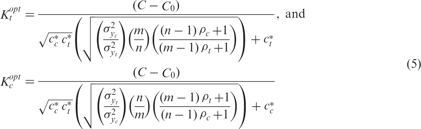
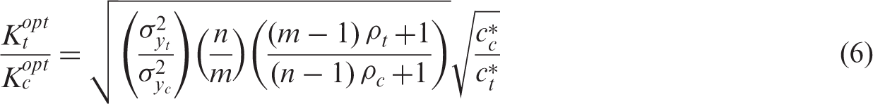
This formula extends the allocation ratio derived by Walwyn and Roberts,⁹ which minimizes the variance for a given total sample size (that is, s_t = s_c = 1 and c_t = c_c = 0 in equation (3)). As can be seen, the number of treatment clusters compared to the number of control clusters increases as a function of the total variance and the intraclass correlation of the treatment condition, and decreases as a function of the cluster size and the cost per cluster in the treatment condition.

For practical purposes, it is useful to transform the optimal numbers of clusters in equation (5) into expressions for numbers of clusters that yield sufficient power for an intervention effect of a particular size. This will be addressed in the next section.

4 Optimal number of clusters for a given power and effect size

The test statistic for the effectiveness of the treatment is ${\overset{\land}{β}}_{1} / \sqrt{v \overset{\land}{a} r ({\overset{\land}{β}}_{1} | ξ)}$ . In case of REML estimation (without truncation of negative estimates of the variance components), the test statistic ${\overset{\land}{β}}_{1} / \sqrt{v \overset{\land}{a} r ({\overset{\land}{β}}_{1} | ξ)}$ can be shown to be identical to a t-test for two independent samples on the cluster means (see supplementary materials for a proof). As a result, when the arms are homogeneous in their intraclass correlation, outcome variance, and cluster size, the test statistic follows Student’s t-distribution with K_t + K_c – 2 degrees of freedom. With heterogeneous variances, intraclass correlations or cluster sizes, the cluster means are very likely to have heterogeneous variances, in which case the test statistic can be approximated by a t-distribution, the degrees of freedom being calculated according to Satterthwaite’s method.¹³ For sufficiently large numbers of clusters (the small K case is covered in section 6), the standard normal is an appropriate reference distribution for this statistic.¹⁴ The relation between the variance of the treatment estimator and the power level 1 – γ to detect a treatment effect in a two-tailed test with type I error rate α, is then approximated by

var ({\overset{\land}{β}}_{1} | ξ) = (\frac{β_{1}}{z_{1 - α / 2} + z_{1 - γ}}) 2

(7)

where z_1–α/2 and z_1–γ are the 100(1 – α/2) and 100(1 – γ) percentiles of the standard normal distribution. Let ψ be the ratio of the variance in the treatment arm versus the variance in the control arm, ψ =

σ_{y_{t}}^{2} / σ_{y_{c}}^{2}

. Furthermore, let ES =

β_{1} / \sqrt{0.5 (σ_{y_{t}}^{2} + σ_{y_{c}}^{2})}

be the effect size based on the variances in the treatment and control arm (cf. Cohen¹⁵). From equations (2) and (7), the optimal number of clusters for the treatment arm that realizes a certain power level 1–γ can then be derived (see Appendix A)

K_{t}^{opt} = \frac{1}{ES 2} (z_{1 - α / α 22} + z_{1 - γ}) 2 \sqrt{\frac{(m - 1) ρ_{t} + 1}{m}} (\sqrt{\frac{(m - 1) ρ_{t} + 1}{m}} + \sqrt{\frac{(n - 1) ρ_{c} + 1}{ψ n} \times \frac{c_{c}^{*}}{c_{t}^{*}}}) (\frac{2 ψ}{ψ + 1})

(8)

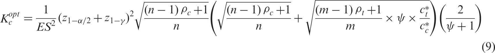
Substituting this expression into equation (6), yields the optimal number of clusters in the control arm, $K_{c}^{opt}$ , for a power level of 1–γ

K_{c}^{opt} = \frac{1}{ES 2} (z_{1 - α / α 22} + z_{1 - γ}) 2 \sqrt{\frac{(n - 1) ρ_{c} + 1}{n}} (\sqrt{\frac{(n - 1) ρ_{c} + 1}{n}} + \sqrt{\frac{(m - 1) ρ_{t} + 1}{m} \times ψ \times \frac{c_{t}^{*}}{c_{c}^{*}}}) (\frac{2}{ψ + 1})

(9)

Equations (8) and (9) show that both $K_{t}^{opt}$ and $K_{c}^{opt}$ increase with ρ_t and ρ_c, whereas $K_{t}^{opt}$ decreases and $K_{c}^{opt}$ increases with $c_{t}^{*} / c_{c}^{*}$ . It should be noted that these effects of the intraclass correlation hold for a given power and ES, since increasing either of the intraclass correlations increases the variance of the treatment effect estimator (see equation (2)). Under a budget constraint on the other hand, increasing one intraclass correlation increases the number of clusters for the corresponding arm at the expense of the number of clusters of the other arm, see equation (6). How the optimal numbers of clusters change when m and n change, with $c_{t}^{*} / c_{c}^{*}$ in equations (8) and (9) changing correspondingly, is somewhat more complicated. Taking the derivative of equation (8) with respect to m and n shows that $K_{t}^{opt}$ always decreases as a function of m, but, as a function of n, is minimum at n = ((c_c/s_c)(1– ρ_c)/ρ_c) ¹ ^/ ² . In a similar way, it can be shown that $K_{c}^{opt}$ always decreases as a function of n, but, as a function of m, takes a minimum at m = ((c_t/s_t)(1– ρ_t)/ ρ_t) ¹ ^/ ² .

For a fixed treatment effect, $β_{1}$ , and a fixed outcome variance summed across both arms, that is, $σ_{y_{t}}^{2}$ + $σ_{y_{c}}^{2}$ , it can further be shown that $K_{t}^{opt}$ and $K_{c}^{opt}$ have a maximum as a function of ψ, with the maximum for $K_{t}^{opt}$ occurring for values ψ ≥ 1 and the maximum for $K_{c}^{opt}$ occurring for values ψ ≤ 1. More precisely, the maximizer for $K_{t}^{opt}$ as a function of ψ is

ψ_{max} = (\frac{(m - 1) ρ_{t} + 1}{(n - 1) ρ_{c} + 1}) \times \frac{n}{m} \times \frac{c_{t}^{*}}{c_{c}^{*}} \times (\sqrt{1 + (\frac{(n - 1) ρ_{c} + 1}{(m - 1) ρ_{t} + 1}) \times \frac{m}{n} \times \frac{c_{c}^{*}}{c_{t}^{*}}} + 1) 2

(10)

and the maximizer for

K_{c}^{opt}

ψ_{max} = (\frac{(n - 1) ρ_{c} + 1}{(m - 1) ρ_{t} + 1}) \times \frac{m}{n} \times \frac{c_{c}^{*}}{c_{t}^{*}} \times (\sqrt{1 + (\frac{(m - 1) ρ_{t} + 1}{(n - 1) ρ_{c} + 1}) \times \frac{n}{m} \times \frac{c_{t}^{*}}{c_{c}^{*}}} - 1) 2

(11)

Figure 1 illustrates the effect of increasing ψ, for a scenario where ES = 0.5 (i.e. a medium sized effect according to Cohen¹⁵). For the range of values shown for ψ, increasing ψ leads to a decrease of $K_{c}^{opt}$ , but first leads to an increase and then to a decrease of $K_{t}^{opt}$ . Again these trends apply under the constraint of a fixed ES and power. When fixing the budget, increasing ψ always leads to an increase of K_t and a decrease of K_c (see equation (6)). Furthermore, in line with equations (8) and (9), for both arms the optimal number of clusters increases as ρ_c increases from 0.01 to 0.30 (ρ_t in both cases being fixed at 0.01 in Figure 1).

Figure 1.

Optimal number of clusters for the treatment and control arm for m = 10, n = 4, ρ_t = 0.01, c_t/s_t = c_c/s_c = 5, s_t/s_c = 0.1, effect size (ES) = 0.5, power = 0.80, and type I error rate = 0.05, as a function of the variance ratio ψ and intraclass correlation in the control arm (ρ_c = 0.01 versus ρ_c = 0.30).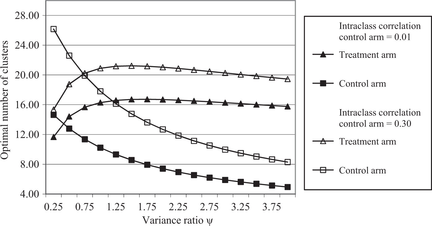

Table 1 presents, for several cost ratios, examples of the optimal numbers of clusters for various values of the variance ratios, cluster sizes m and n, and intraclass correlations (i.e. ρ_t = ρ_c = 0.01 and ρ_t = ρ_c = 0.30). Following Raudenbush¹ and Van Breukelen and Candel,¹⁶ we consider the cost ratios c_t/s_t and c_c/s_c to vary between 2 and 50, and, in line with Liu,¹¹ s_t/s_c varies between 1/10 and 10. Employing the standard normal distribution as the reference distribution for the test statistic, optimal cluster numbers are given for 80% power for a medium ES, that is, ES = 0.5. As can be seen, the variation in optimal cluster numbers is rather large and depends on the different parameters in the way as delineated above. For example, the optimal numbers of clusters are always larger for larger intraclass correlations. Also, increasing m and n, respectively, leads to decrease in

K_{t}^{opt}

and

K_{c}^{opt}

. It can also be seen that the optimal allocation ratio of treatment and control clusters may clearly deviate from one, contrasting with common practice.^7,17–19

Table 1.

Optimal cluster numbers for different cost ratios, variance ratios, cluster sizes m and n, and different intraclass correlations, for an effect size ES = 0.50, assuming a power of 80% and a two-tailed test with type I error rate α = 0.05.

							ρ_t = 0.01_; ρ_c = 0.01		ρ_t = 0.30_; ρ_c = 0.30
c_t/s_t	c_c/s_c	s_t/s_c	c_t/c_c	ψ	m	n	$K_{t}^{opt}$	$K_{c}^{opt}$	$K_{t}^{opt}$	$K_{c}^{opt}$
2	2	0.1	0.1	0.25	4	4	24	15	44	28
2	2	0.1	0.1	0.25	4	16	22	5	62	20
2	2	0.1	0.1	0.25	16	4	8	15	23	30
2	2	0.1	0.1	0.25	16	16	7	5	34	20
2	2	0.1	0.1	4	4	4	34	6	62	10
2	2	0.1	0.1	4	4	16	32	2	80	7
2	2	0.1	0.1	4	16	4	10	6	36	12
2	2	0.1	0.1	4	16	16	10	2	45	8
50	2	0.1	2.5	0.25	4	4	11	20	19	36
50	2	0.1	2.5	0.25	16	4	5	17	14	35
50	2	0.1	2.5	0.25	4	16	10	6	25	23
50	2	0.1	2.5	0.25	16	16	4	5	19	23
50	2	0.1	2.5	4	4	4	20	10	37	18
50	2	0.1	2.5	4	16	4	7	7	27	17
50	2	0.1	2.5	4	4	16	20	3	43	10
50	2	0.1	2.5	4	16	16	7	2	32	10
50	2	2	50	0.25	4	4	5	41	9	75
50	2	2	50	0.25	16	4	2	29	7	72
50	2	2	50	0.25	4	16	5	12	11	43
50	2	2	50	0.25	16	16	2	9	8	41
50	2	2	50	4	4	4	15	31	27	57
50	2	2	50	4	16	4	5	20	20	54
50	2	2	50	4	4	16	15	10	28	30
50	2	2	50	4	16	16	5	6	21	28
50	50	0.1	0.1	0.25	4	4	24	15	44	28
50	50	0.1	0.1	0.25	16	4	11	15	34	28
50	50	0.1	0.1	0.25	4	16	16	5	42	21
50	50	0.1	0.1	0.25	16	16	7	5	32	20
50	50	0.1	0.1	4	4	4	34	6	62	10
50	50	0.1	0.1	4	16	4	14	5	47	10
50	50	0.1	0.1	4	4	16	25	2	60	8
50	50	0.1	0.1	4	16	16	10	2	45	8

Table 1 furthermore illustrates that the optimal number of clusters for one of the arms may become larger than feasible. In these cases, the number of clusters in this arm could be reduced to the largest number that is feasible, and the number of clusters in the other arm then needs to be increased such that the power level is maintained according to equations (2) and (7). This would then be the most cost-efficient feasible design.

Calculation of optimal designs yielding sufficient power requires knowledge of relevant model parameters such as the intraclass correlations ρ_t and ρ_c and the variance ratio ψ. Since there will rarely be precise knowledge on these parameters, in the next section, we will discuss the maximin design as a possible solution.

5 Uncertainty on model parameters: Maximin designs

To calculate the optimal cluster numbers by equations (8) and (9), we need to specify the values of the intraclass correlations ρ_t and ρ_c and the value of ψ, on which we may have no precise prior knowledge. A rather straightforward solution is the maximin strategy.²⁰ The maximin strategy consists of the following two steps: (1) for each design determine the minimum efficiency of the treatment effect estimator across the range of plausible values for the intraclass correlations and variance ratio ψ, and (2) choose that design, which, given the budget, maximizes this minimum efficiency. This design optimizes a worst case scenario and is known as the maximin design. Since efficiency is the inverse of the variance of the treatment estimator, the maximin strategy implies choosing that design which minimizes the maximum variance of the treatment effect estimator. This is practically useful because, in sample size calculation, choosing values for the intraclass correlations and the variance ratio which maximize the variance of the treatment estimator, will guarantee a desired power level also for all other values of these parameters within their plausible ranges. The maximin design is obtained by filling in these worst case intraclass correlations and variance ratio in equations (8) and (9), and thereby guarantees the power level under the worst case scenario at the lowest costs.

Taking the derivative of equation (2) with respect to ρ_t and ρ_c shows that the variance of the treatment effect estimator increases as a function of both ρ_t and ρ_c. The maximin design therefore should be based on the upper boundaries of the plausible ranges for these parameters. Keeping the total outcome variance, that is $σ_{y_{t}}^{2}$ + $σ_{y_{c}}^{2}$ , constant, we furthermore show in Appendix B that the variance of the treatment estimator in the maximin design is maximized by the following value of ψ

ψ_{max} = (\frac{(m - 1) ρ_{t} + 1}{m}) (\frac{n}{(n - 1) ρ_{c} + 1}) \frac{c_{t}^{*}}{c_{c}^{*}}

(12)

If the range of plausible values for ψ comprises equation (12), then this value should be chosen, if the range is below the value in equation (12), then the upper boundary of the range should be chosen, and if the range is above the value in equation (12), then the lower boundary of the range should be chosen. These choices give the maximum variance of the treatment estimator in equation (2), and therefore yield safe sample sizes by equations (8) and (9).

Note that equations (8) and (9) are based on the standard normal as a reference distribution for the test statistic. Hence, when small numbers of clusters result, corrections may be needed of these cluster numbers to obtain the desired power level. This issue will be addressed in the next section.

6 Corrections for the numbers of clusters as based on the normal approximation

The sample size calculations in equations (8) and (9) are based on the standard normal approximation of the test statistic. In case the treatment arms have equal outcome variances, equal intracluster correlations and equal cluster sizes, so that the variance of cluster outcome means is homogeneous between arms, numerical evaluations for 80% and 90% power show that, for K_t = K_c varying from five to 50, adding one cluster to K_t and K_c each, is a sufficient correction for two-tailed tests with a 5% type I error rate. Adding two clusters to K_t and K_c each turns out to be a sufficient correction for a 1% type I error rate.¹⁶

In case the outcome variances, intracluster correlations or cluster sizes are not the same across both treatment arms, an adequate approximation of the distribution of the test statistic, provided each treatment arm contains at least four clusters,^13,21 is the t-distribution with degrees of freedom given by the Satterthwaite approximation. Employing an exact expression for the power of this Satterthwaite approximation,²² a numerical evaluation for heterogeneous treatment arms was done to determine appropriate corrections of the number of clusters. Since the numerical evaluation has to be based on realistic ranges for each of the parameters in equations (8) and (9), these parameter ranges will be addressed first.

6.1 Choice of ranges for relevant model parameters

6.1.1 Intraclass correlations

The intraclass correlations, ρ_t and ρ_c, range from 0.01 to 0.30, since this represents the range commonly encountered in trials comparing group administered interventions^2,3,8 or trials where clustering effects are due to therapists.^3,23

6.1.2 Ratio of outcome variances

Since there is not much empirical evidence on ψ, with one study indicating that it varies between 0.5 and 2,⁷ we will examine a somewhat broader range: ψ runs from 0.25 to 4.

6.1.3 Cluster sizes

In individually randomized group treatments as well as in case of individual treatments with clustering due to shared therapist effects, the cluster sizes are often rather small. The smallest average group size encountered in group therapy is about four,^8,19,24 whereas 10 seems to be an upper limit.^7,18,25 These cluster sizes also encompass the average numbers of patients commonly treated within the same period by one therapist,^23,26,27 although the maximum seems to be somewhat larger.^28,29 A cluster size of 16 will therefore be considered as an upper limit.

6.1.4 Effect sizes

The ES varies between 0.1 and 0.9, thus encompassing the ESs commonly classified as small (i.e. 0.2), medium (i.e. 0.5), and large (i.e. 0.80).¹⁵

6.1.5 Cost ratios

The empirical evidence on the costs c_t, c_c, s_t, and s_c is rather scarce, an exception being for instance Moerbeek et al.³⁰ (where c_t/s_t = c_c/s_c = 26). To obtain general results, we therefore did not constrain the number of clusters through the cost function in equation (4). Instead K_t and K_c were varied from two to 140, such that they yielded 80% or 90% power in a two-tailed test with a 5% or 1% type I error rate.

6.2 Numerical investigation

First, all different combinations of ρ_t, ρ_c, ψ, m, n, ES, and K_c were generated within the ranges of these parameters as described in section 6.1. To obtain K_t that, given the values of the other parameters, yields a power level 1 – γ in a two-tailed test with type I error rate α, equations (2) and (7) are combined to obtain the following expression for K_t

K_{t} = \frac{(z_{1 - α / α 22} + z_{1 - γ}) 2 (\frac{(m - 1) ρ_{t} + 1}{m}) ψ K_{c}}{0.5 \times ES 2 (ψ + 1) K_{c} - (z_{1 - α / α 22} + z_{1 - γ}) 2 (\frac{(n - 1) ρ_{c} + 1}{n})}

(13)

Second, it was checked whether adding a certain number of clusters to the treatment arms is sufficient for yielding a required power level, as evaluated by an exact expression for the power.²² For this check a program in R was written.³¹ For some values of the parameters, the integral function in R did not yield a finite value, in which case 200.000 Monte Carlo simulations were done to evaluate the power level.

A simple correction was determined in which an equal number of clusters was added to both treatment arms. More precisely, the smallest number of clusters was determined that, when added to both treatment arms, was sufficient for all possible combinations of ρ_t, ρ_c, ψ, m, n, ES, K_c, and K_t. Let us denote this smallest number by k. Next, refinements of this correction were determined. As a first step, the smallest K_t and smallest K_c were sought for, for which the (same) number of clusters added to each arm could be reduced to k – 1. Denote this smallest K_t and K_c by K₁. The result of this process is visualized in Figure 2. To find K₁, a binary search algorithm was used.³² If K₁ had been found, then a second binary search was done to find the smallest K_t and smallest K_c for which the number of clusters added could be reduced to k–2 for both arms. Denote this smallest K_t and K_c by K₂ (where K₂ > K₁). These binary searches where repeated until either a smallest K_t and smallest K_c was found for which no correction to equation (13) was necessary anymore, or no correction turned out to be sufficient for the required power level even for a K_t and K_c of 140.

Figure 2.

Graphical display of sufficient corrections in terms of adding the same number of clusters to K_t and K_c as a function of the minimum of K_t and K_c. The ranges for K_t and K_c run from two to 140. If both K_t and K_c are K₁ or larger at most k–1 clusters have to be added to K_t and to K_c (k–1,k–1). If both K_t and K_c are K₂ or larger at most k–2 clusters have to be added to K_t and to K_c (k–2,k–2).

In a second step, these corrections were further refined as a function of the maximum of K_t and K_c. More precisely, consider the area in Figure 2 for which adding k–1 clusters (but not k–2 clusters) to each arm was sufficient, that is, K_t in [K₁,K₂–1] and K_c in [K₁,140] or K_c in [K₁,K₂–1] and K_t in [K₁,140]. For this area, it was examined through a binary search, at which smallest value of the largest of K_t and K_c, the number of clusters added to the largest of K_t and K_c could be one less (that is, k–2 instead of k–1). If this smallest value was found, say K₃, next for the area where K_t in [K₁,K₂–1] but K_c in [K₃,140] or K_c in [K₁,K₂–1] but K_t in [K₃,140] (see Figure 2), a binary search was done to determine the smallest maximum of K_t and K_c for which the number of clusters added to the largest arm could be further reduced by one (that is, k–3). This refinement was carried out for each correction area as established before (the areas defined by K₁ and K₂ in Figure 2).

6.3 Results from the numerical evaluation

For K_t and K_c varying from two to 140, it appears that adding three clusters to K_t and K_c each, is a sufficient correction in case of two-tailed test at a 5% type I error rate. For a two-tailed test at a 1% type I error rate, adding four clusters to K_t and K_c each turns out to be sufficient. These corrections can be relaxed somewhat in case of larger cluster numbers. Table 2(a) and (b) shows sufficient corrections of the cluster numbers as a function of the minimum of K_t and K_c on one hand and the maximum of K_t and K_c on the other. These refinements in corrections guarantee a power level up to 0.5%, that is, at least 79.5% and 89.5% for the power levels 80% and 90%, respectively. As an example, for 80% power and a 5% type I error rate adding two clusters to each arm are sufficient corrections when the minimum of K_t and K_c according to equations (8) and (9) exceeds seven (see Table 2(a)). Furthermore, if one of K_t and K_c exceeds 68, then for this arm it suffices to add only one cluster. For the same power level but a 1% type I error rate, it suffices to add three clusters to each arm if the minimum of K_t and K_c exceeds 25 (see Table 2(b)). If also one of K_t and K_c exceeds 89, then for this arm only two clusters need to be added.

Table 2(a).

The extra number of clusters to be added to each treatment arm (to the minimum and to the maximum number of clusters), both printed bold within parentheses, when calculating the cluster numbers according to the standard normal approximation in equations (8) and (9) and when employing REML estimation in the linear mixed model analysis.

Type I error rate = 5%
Power = 0.80			Power = 0.90
Minimum of K_t and K_c	Maximum of K_t and K_c		Minimum of K_t and K_c	Maximum of K_t and K_c
2–4	2–4	(+ 3, + 3)	2–3	2–3	(+ 3, + 3)
2–7	5–18	(+ 3, + 2)	2–6	4–17	(+ 3, + 2)
2–7	19–28	(+ 3, + 1)	2–6	18– 26	(+ 3, + 1)
2–7	29–140	(+ 3, + 0)	2–6	27–140	(+ 3, + 0)
8–68	8–68	(+ 2, + 2)	7–53	7–140	(+ 2, + 2)
8–74	69–138	(+ 2, + 1)	54–104	54–119	(+ 1, + 1)
8–74	139–140	(+ 2, + 0)	54–104	120–140	(+ 1, + 0)
75–140	75–140	(+ 1, + 1)	105–140	105–140	(+ 0, + 0)

Below we will illustrate how optimal and maximin sample sizes can be calculated for a specific study, and will also illustrate the benefits of using a maximin design as compared to a design with equal numbers of clusters in each arm.

7 Application in planning a trial

We illustrate how to use the results of the present study when planning a trial with heterogeneous clustering in the treatment arms. Baldwin et al.⁷ studied the effects of two group-administered interventions (dissonance intervention versus a healthy weight management program), administered to high school and university students expressing body image concerns. In this study, a central outcome was the score on the Revised Ideal Body Stereotype Scale, a self-report measure of internalization of the thin beauty ideal. Equations (8) and (9) can be used to calculate the numbers of clusters when replicating this study. We set s_t = s_c = 1 and c_t = c_c = 0 in equation (3) so that the total sample size is minimized and we take the parameter estimates from Baldwin et al.,⁷ that is, $\overset{\land}{ψ}$ = 0.78, ${\overset{\land}{ρ}}_{t}$ = 0.04, and ${\overset{\land}{ρ}}_{c}$ = 0.25, as best guesses as to the true parameter values. If we want to detect a medium sized effect of the intervention, that is, ES = 0.5 (cf. Cohen¹⁵), with 80% power at a 5% type I error rate in a two-tailed test, and m = n = 6 are ideal group sizes for both arms (cf. Baldwin et al.⁷), then K_t = 15 groups are needed for the treatment arm (by equation (8)) and K_c = 22 groups for the other arm (by equation (9)). To repair the power loss due to using the standard normal instead of the t-distribution in calculating K_t and K_c, these numbers should be increased to K_t = 15 + 2 = 17 and K_c = 22 + 2 = 24 groups, respectively (see Table 2(a)).

If one wants to be on the safe side, the maximin strategy can be used, and 0.10 and 0.30 could be chosen as upper boundaries for ρ_t and ρ_c, respectively. Substituting these into equation (12) shows that the variance of the treatment estimator is maximum at ψ = 0.6. If this value is within the plausible range of values for ψ, then, by using equations (8) and (9), the maximin sample sizes can be calculated as: K_t = 16 and K_c = 27. Accounting again for the power loss due to using the standard normal distribution for the test statistic, this should be increased to K_t = 16 + 2 = 18 and K_c = 27 + 2 = 29 groups, respectively (see Table 2(a)). Calculations of the number of clusters according to an optimal design or a maximin design, also including the corrections as displayed in Table 2(a) and (b), are possible via a small menu-driven program written in R (CLUSCALCRT),³¹ which, upon request, is available from the first author.

Finally, if one wants to replicate the study of Baldwin et al.,⁷ one could start from a maximin strategy with ρ_t = 0.10, ρ_c = 0.30 and ψ = 0.6, and compare the maximin design to a design where K_t = K_c, as typical for many studies^7,17–19. Since we do not have information on the research costs, different cost ratios are considered. Columns 5 and 6 of Table 3 show the relative gains in budget when considering a maximin design as compared to a design with K_t = K_c in case both designs have 80% or 90% power at ES = 0.50 in a two-tailed test with a 5% type I error rate. The budget gains can become as large as 50%, illustrating that there may be clear monetary benefits for a maximin design. Further, columns 7 and 8 of Table 3 show the gains in power under identical budgets when considering a maximin design as compared to a design with K_t = K_c which has either 80% or 90% power at ES = 0.50 in a two-tailed test with a 5% type I error rate. The power gains may be up to nearly 20% for an 80% power level and up to 10% for a 90% power level of the equal allocation design. This implies that for some cost ratios the power levels for the maximin design are close to 100% for the same budget as the equal allocation design. Note furthermore that there also may be some small budget and power losses for the maximin design. This is due to rounding of the cluster numbers and due to the corrections as displayed in Table 2(a) and (b) being sufficient but not necessary.

Table 2(b).

Type I error rate = 1%
Power = 0.80			Power = 0.90
Minimum of K_t and K_c	Maximum of K_t and K_c		Minimum of K_t and K_c	Maximum of K_t and K_c
2–17	2–17	(+ 4, + 4)	2–14	2–14	(+ 4, + 4)
2–25	18–47	(+ 4, + 3)	2–21	15–35	(+ 4, + 3)
2–25	48–64	(+ 4, + 2)	2–21	36– 57	(+ 4, + 2)
2–25	65–93	(+ 4, + 1)	2–21	58–81	(+ 4, + 1)
2–25	94–140	(+ 4, + 0)	2–21	82–140	(+ 4, + 0)
26–89	26–89	(+ 3, + 3)	22–70	22–70	(+ 3, + 3)
26– 94	90–139	(+ 3, + 2)	22–73	71–131	(+ 3, + 2)
26– 94	140–140	(+ 3, + 1)	22–73	132–140	(+ 3, + 1)
95–140	95–140	(+ 2, + 2)	74–132	74–139	(+ 2, + 2)
			74–132	140–140	(+ 2, + 1)
			133–140	133–140	(+ 1, + 1)

Table 3.

Budget and power of the maximin design versus an equal allocation design (K_t = K_c) for different cost ratios and power levels.

				Relative budget gain under equal power levels Power for equal allocation and maximin design		Absolute power gain under equal budgets Power for equal allocation design
c_t/s_t	c_c/s_c	s_t/s_c	c_t/c_c	80%	90%	80%	90%
2	2	0.1	0.1	2%	3%	2%	6%
2	2	1	1	4%	4%	2%	6%
2	2	10	10	40%	41%	16%	10%
2	20	0.1	0.01	11%	10%	4%	7%
2	20	1	0.1	–2%	–2%	–1%	5%
2	20	10	1	19%	21%	9%	8%
20	2	0.1	1	–1%	–1%	–1%	5%
20	2	1	10	20%	23%	9%	9%
20	2	10	100	50%	53%	19%	10%
20	20	0.1	0.1	2%	3%	2%	6%
20	20	1	1	4%	4%	2%	6%
20	20	10	10	40%	41%	16%	10%

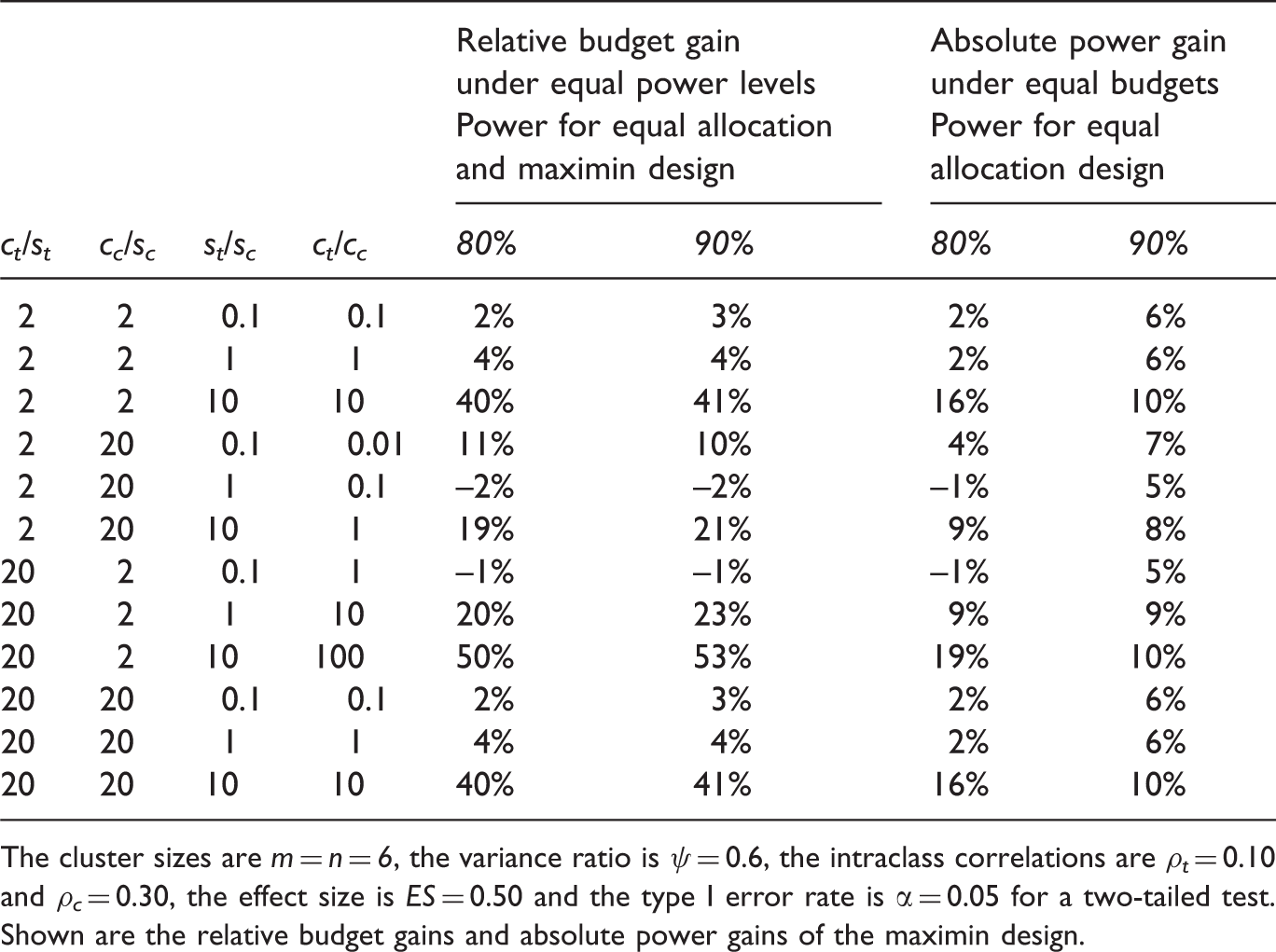
The cluster sizes are m = n = 6, the variance ratio is ψ = 0.6, the intraclass correlations are ρ_t = 0.10 and ρ_c = 0.30, the effect size is ES = 0.50 and the type I error rate is α = 0.05 for a two-tailed test. Shown are the relative budget gains and absolute power gains of the maximin design.

8 Conclusions and discussion

Clustering may occur when comparing group administered treatments, such as group wise psychotherapy where group members influence each other, or when comparing individual treatments where individuals are nested within care providers, such as psychotherapists, and provider effects occur. Starting from a priori fixed and constant cluster sizes and employing a flexible cost function, we derived the numbers of clusters that minimize the variance of the treatment effect estimator. This generalizes previous studies in that allowance is made for between-arm differences in the intraclass correlation, outcome variance, cluster size, number of clusters, and costs. The optimal number of clusters for a treatment arm may vary to a large extent (from two to more than 70) and the optimal allocation of clusters to the treatment arms may clearly deviate from a 50-50 allocation. Calculating optimal sample sizes requires prior knowledge on the intraclass correlations in both arms and on the between-arm ratio of outcome variances, which often may not be very precise. To accommodate this, a maximin strategy for calculating sample sizes was presented. Maximin sample sizes guarantee a desired power level at the lowest costs for all parameter values in their plausible ranges. Since the power of any design, including an optimal or a maximin design, also depends on the ES of interest, expressions were furthermore given for calculating the number of clusters needed for a certain power level and ES. As these equations were based on the normal approximation of the test statistic, a numerical study was done which showed that for both 80% and 90% power, increasing the number of clusters in each arm by either three or four clusters was sufficient to obtain the required power level for type I error rates of 5% and 1%, respectively.

For some care providers, such as nurse practitioners or general practitioners, the intervention often involves a single or a few meetings of limited duration, implying that the average number of patients per care provider may be much larger than considered in the present numerical study (see e.g. Roberts and Roberts,³ Roth et al.³³). Additional numerical evaluations with larger average cluster sizes could be done to examine whether similar corrections result in this case.

The methodology of the present paper could also be applied to designs where the number of clusters are fixed. That is, it is also possible to derive the optimal cluster sizes, for fixed numbers of clusters in the treatment and control arm, by minimizing the variance of the treatment effect estimator for a given budget. However, it may not be possible to find optimal cluster sizes needed for achieving a certain power level, as the variance of the treatment effect estimator does not become arbitrarily small as m and n approach infinity, except if both intraclass correlations are zero (see equation 2). Stated otherwise, given fixed numbers of clusters in the treatment and control arm, there may be no optimal m and n realizing a desired power level for a particular ES.

Since the sample size formulas assume constant cluster sizes, whereas varying cluster sizes, due to dropout or naturally varying group sizes, is the more common case, one relevant extension of the paper is examining the effect of varying cluster sizes on the design efficiency and deriving a correction for the potential efficiency loss in a cost-efficient way when planning sample sizes. Van Breukelen et al.³⁴ have shown that in many cases adding about 10% of the clusters to both arms compensates the efficiency loss due to varying cluster sizes, but this result applies to arms that are homogeneous in their intraclass correlation, outcome variance, number of clusters and average cluster size. Formulating correction guidelines for the efficiency loss for designs where there is between-arms heterogeneity in these features requires deriving the efficiency loss for the asymptotic case and evaluating the adequacy of this asymptotic result for finite samples through an extensive Monte Carlo simulation study. This extension will be addressed in an upcoming paper.

Footnotes

Funding

This research received no specific grant from any funding agency in the public, commercial, or not-for-profit sectors.

Conflict of interest

None declared.

Appendix A: Optimal cluster numbers for fixed cluster sizes in case of ML estimation of the treatment effect

Appendix B: Value of ψ which maximizes the variance of the treatment effect estimator for maximin designs

References

Raudenbush

. Statistical analysis and optimal design for cluster randomized trials. Psychol Meth 1997; 2: 173–185.

Baldwin

Murray

Shadish

. Empirically supported treatments or type I errors? Problems with the analysis of data from group-administered treatments. J Consult Clin Psychol 2005; 73: 924–935.

Roberts

. The design and analysis of clinical trials with clustering effects due to treatment. Clin Trials 2005; 2: 152–162.

Pals

Murray

Alfano

. Individually randomized group treatment trials: a critical appraisal of frequently used design and analytic approaches. Am J Public Health 2008; 98: 1418–1424.

Dannon

Gon-Usishkin

Gelbert

. Cognitive behavioral group therapy in panic disorder patients: the efficacy of CBGT versus drug treatment. Ann Clin Psychiatry 2004; 16: 41–46.

Otto

Pollack

Gould

. A comparison of the efficacy of clonazepam and cognitive-behavioral group therapy for the treatment of social phobia. J Anxiety Disord 2000; 14: 345–358.

Baldwin

Stice

Rohde

. Statistical analysis of group-administered intervention data: reanalysis of two randomized trials. Psychother Res 2008; 18: 365–376.

Tasca

Illing

Ogrodniczuk

. Assessing and adjusting for dependent observations in group treatment research using multilevel models. Group Dynam 2009; 13: 151–162.

Walwyn

Roberts

. Therapist variation within randomized trials of psychotherapy: implications for precision, internal and external validity. Stat Methods Med Res 2010; 19: 291–315.

10.

Moerbeek

Van Breukelen

GJP

Berger

MPF

. Design issues for experiments in multilevel populations. J Educ Behav Stat 2000; 25: 271–284.

11.

Liu

. Statistical power and optimum sample allocation ratio for treatment and control having unequal costs per unit of randomization. J Educ Behav Stat 2003; 28: 231–248.

12.

Demidenko

. Mixed models: theory and applications, New Jersey: Wiley, 2004.

13.

Davenport

Webster

. Type-I error and power of a test involving a Satterthwaite’s approximate F-statistic. Technometrics 1972; 14: 555–569.

14.

Dixon

Massey

. Introduction to statistical analysis, New York: McGraw Hill, 1983.

15.

Cohen

. A power primer. Psychol Bull 1992; 112: 155–159.

16.

Van Breukelen

GJP

Candel

MJJM

. Sample sizes for cluster randomized trials: we can keep it simple and efficient!. J Clin Epidemiol 2012; 65: 1212–1218.

17.

Herzog

Lazev

Irvin

. Testing for group membership effects during and after treatment: the example of group therapy for smoking cessation. Behav Ther 2002; 33: 29–43.

18.

Hoover

. Clinical trials of behavioral interventions with heterogeneous teaching subgroup effects. Stat Med 2002; 21: 1351–1364.

19.

Tasca

Illing

Joyce

. Three-level multilevel growth models for nested change data: a guide of group treatment researchers. Psychother Res 2009; 19: 453–461.

20.

Atkinson

Donev

Tobias

. Optimum experimental designs, with SAS, Oxford: Oxford University Press, 2007.

21.

Davenport

Webster

. The Behrens-Fisher problem, an old solution revisited. Metrika 1975; 22: 47–54.

22.

Moser

Stevens

Watts

. The two-sample t test versus Satterthwaite’s approximate F test. Comm Stat Theor Meth 1989; 18: 3963–3975.

23.

De Jong

Moerbeek

Van der Leeden

. A priori power analysis in longitudinal three-level multilevel models: an example with therapist effects. Psychother Res 2010; 20: 273–284.

24.

Newton-John

TRO

Spence

Schotte

. Cognitive-behavioral therapy versus EMG feedback in the treatment of chronic low-back-pain. Behav Res Ther 1995; 33: 691–697.

25.

Imel

Baldwin

Bonus

. Beyond the individual: group effects in mindfulness-based stress reduction. Psychother Res 2008; 18: 735–742.

26.

Thompson

Gallagher

Breckenridge

. Comparative effectiveness of psychotherapies for depressed elders. J Consult Clin Psychol 1987; 55: 385–390.

27.

Wampold

Serlin

. The consequence of ignoring a nested factor on measures of effect size in analysis of variance. Psychol Meth 2000; 5: 425–433.

28.

Crits-Cristoph

Mintz

. Implications of therapist effects for the design and analysis of comparative studies of psychotherapies. J Consult Clin Psychol 1991; 59: 20–26.

29.

Durham

Murphy

Allan

. Cognitive therapy, analytic psychotherapy and anxiety management training for generalized anxiety disorder. Br J Psychiatry 1994; 165: 315–323.

30.

Moerbeek

Van Breukelen

GJP

Berger

MPF

. Optimal sample sizes in experimental designs with individuals nested within clusters. Understand Stat 2003; 2: 151–175.

31.

R Core Team. R: A language and environment for statistical computing. Vienna: R Foundation for Statistical Computing, http://www.R-project.org/ (2013, accessed 20 November 2014).

32.

Cormen

Leiserson

Rivest

. Introduction to algorithms, Cambridge, MA: MIT Press, 2009.

33.

Roth

Rogowski

Yanay

. Teleconsultation for cardiac patients: a comparison between nurses and physicians. The SHL experience in Israel. Telemed J E Health 2006; 12: 528–534.

34.

Van Breukelen

GJP

Candel

MJJM

Berger

MPF

. Relative efficiency of unequal versus equal cluster sizes in cluster randomized and multicentre trials. Stat Med 2007; 26: 2589–2603.

35.

Candel

MJJM

Van Breukelen

GJP

. Varying cluster sizes in trials with clusters in one treatment arm: sample size adjustments when testing treatment effects with linear mixed models. Stat Med 2009; 28: 2307–2324.