Combined dynamic predictions using joint models of two longitudinal outcomes and competing risk data

Abstract

Nowadays there is an increased medical interest in personalized medicine and tailoring decision making to the needs of individual patients. Within this context our developments are motivated from a Dutch study at the Cardio-Thoracic Surgery Department of the Erasmus Medical Center, consisting of patients who received a human tissue valve in aortic position and who were thereafter monitored echocardiographically. Our aim is to utilize the available follow-up measurements of the current patients to produce dynamically updated predictions of both survival and freedom from re-intervention for future patients. In this paper, we propose to jointly model multiple longitudinal measurements combined with competing risk survival outcomes and derive the dynamically updated cumulative incidence functions. Moreover, we investigate whether different features of the longitudinal processes would change significantly the prediction for the events of interest by considering different types of association structures, such as time-dependent trajectory slopes and time-dependent cumulative effects. Our final contribution focuses on optimizing the quality of the derived predictions. In particular, instead of choosing one final model over a list of candidate models which ignores model uncertainty, we propose to suitably combine predictions from all considered models using Bayesian model averaging.

Keywords

Model averaging joint models individualized risk predictions longitudinal data analysis survival analysis

1. Introduction

Motivated by the current increased medical interest in personalized medicine, we focus in this work on subject-specific survival predictions.^1–5 For example, in the field of cardio-thoracic surgery and especially after a heart valve replacement, the main disadvantage of human tissue valve allografts is their limited durability, due to calcification with tissue damage resulting in degeneration and dysfunction. Thus, it may be of interest for the treating physicians to develop a prognostic tool that could inform them about a future re-intervention to their patients using all available repeated measurements. Specifically, the motivation comes from a study that was conducted in the Erasmus Medical Center, Rotterdam, The Netherlands. This study includes 270 patients who received a human tissue valve allograft in aortic position in the Department of Cardio-Thoracic Surgery in a period of 21 years. Patients were followed prospectively over time and measurements of aortic gradient and aortic regurgitation were obtained at six months and one year postoperatively and biennially thereafter.⁶ The continuous variable aortic gradient measures whether the opening of the aortic valve is narrowed, while the ordinal variable aortic regurgitation measures leakage of the aortic valve and consists of five categories. Furthermore, at the end of follow-up, 57 (20.1%) patients had died and 74 (26.1%) patients required a reoperation on the allograft. Since aortic gradient and aortic regurgitation are both measuring aortic heart valve abnormalities and therefore, the presence of one disease will have an influence on the other, it is of great interest from the clinical point of view to analyze them together. In Figure 1, we present the profiles of aortic gradient for males and females, while in Table 1 we present some extra information regarding the data.

Figure 1.

Profile plots of aortic gradient for males and females. The three patients that are highlighted will be used for prediction.

Table 1.

Descriptive statistics.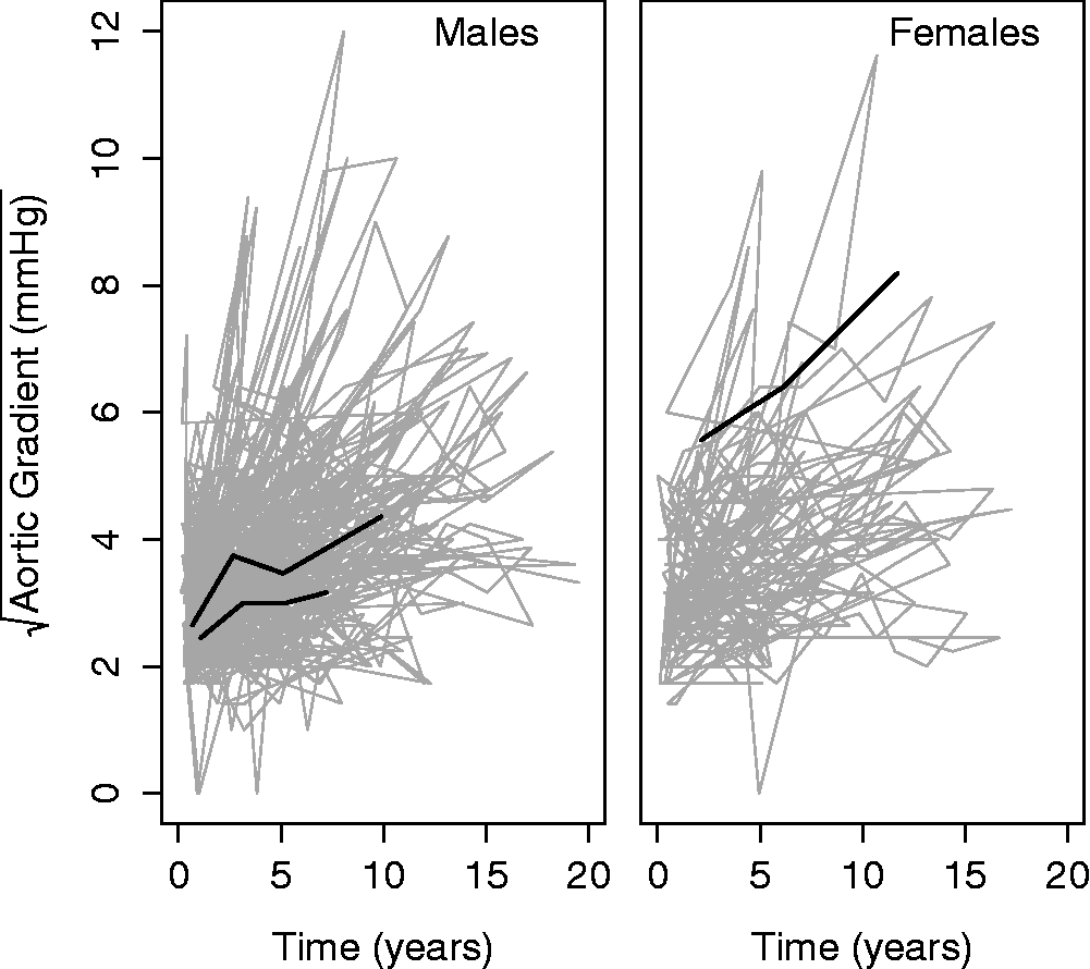

	Mean, sd or %
Age	45.6,14.9
Sex
Males	72
Females	28
Type of operation
Root replacement	73
Subcoronary implantation	27
Merfan
Yes	5
No	95
LVfunction
1	75
2	18
3	2
4	4
Donor age	55.8, 17
Diameter (mm)	22.7, 1.9
Baseline aortic gradient	11.2, 7
Baseline aortic regurgitation
none	13
trace	19
1+	44
2+	19
3+	4

To evaluate the predictive value of the heart valve data on mortality and reoperation and to derive the subject-specific predictions, we rely on joint models for longitudinal and time-to-event data. Joint modeling is an active area of statistics research that has received a lot of attention in recent years.^7–9 Moreover, these models can be used to objectively extract information from multiple markers and to employ them to dynamically update risk estimates. An advantage is that the predictions are updated as more measurements become available. Thus, the statistical predictions can be combined with the physician’s expertise to yield improved health outcomes eventually.

In this paper, we extend the work presented in Andrinopoulou et al.¹⁰ that focuses on fitting the data using a joint model where the survival outcomes are associated with the random effects of the longitudinal outcomes. In particular, our contribution is two-fold: first, we postulate joint models assuming different functional forms to underlie the relationship between multiple longitudinal and survival outcomes and second, we focus on prediction models in the presence of competing risks. Since we are more interested in predicting future patients than simply assessing the degree of association between the trend of the repeated outcomes and time-to-events, it is important to accurately determine the estimate of the underlying process of the heart disease. Thus, we go beyond the standard joint model that utilizes only the latent value of the biomarkers and investigate whether the risk of an event could be affected also by the slope or a summary of the whole history of the longitudinal outcomes.

Finally, it is common practice that a model upon which the clinical predictions are based is selected from a set of different possible models. However, such an approach neglects model uncertainty. In addition, different models may produce more accurate predictions for different types of patients. To explicitly account for these issues we rely on a Bayesian model averaging (BMA) approach.^11,12 More specifically, we propose to suitably combine predictions from joint models that assume different covariates and association structures between the longitudinal and event time processes. Previous research using that approach¹² has focused on BMA risk predictions for one event based on one continuous longitudinal outcome. In this paper, we extend this idea to the competing risk setting while also allowing for multiple longitudinal outcomes. Specifically, motivated by the heart valve study where treating physicians are more interested in risk predictions separately for reoperation and death, we derive a BMA version of the cumulative incidence functions of the two events.

The rest of the paper is organized as follows: Section 2 describes the joint submodels and the Bayesian estimation procedure, Section 3 provides the individualized prediction mechanism and the BMA approach, Section 4 presents the results of the valve data, while Section 5 a simulation study. Finally, in Section 6 we close with a discussion.

2. Methods

2.1 Submodels

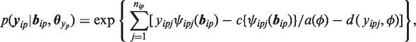
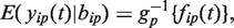
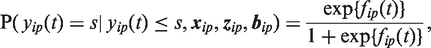
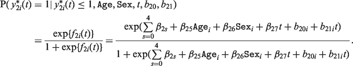
Let $T_{ki}^{*}$ denote the true failure time for the i-th individual ( $i = 1, \dots, n$ ) for each competing event $k = 1, 2, \dots, K$ , and C_i the censoring time, then $T i = min (T_{1 i}^{*}, \dots, T_{Ki}^{*}, C i)$ represents the observed failure time for the i-th patient. Moreover, $δ i = 0, 1, 2, \dots, K$ is the event indicator where 0 indicates censoring. For the longitudinal part, we let $y i = (y_{i 1}^{⊤}, \dots, y_{iP}^{⊤}) ⊤$ and $p = 1, \dots, P$ denote a vector of P outcomes for the i-th patient, where $y ip$ consists of longitudinal responses that may be obtained at different time points $t ij, p$ and have length n_ip. To describe the subject-specific evolutions over time of the longitudinal outcomes, we utilize generalized linear mixed-effects models. In particular, the conditional distribution of the data, given the random effects, is taken to be member of the exponential family of distributions with mean conditional on the random effects

E (y ip (t) | b ip) = g_{p}^{- 1} {f ip (t)},

where

g_{p}^{- 1} (.)

is the inverse link function and

f ip (.)

describes the longitudinal profile for the p-th outcome

f ip (t) = x_{ip}^{⊤} (t) β p + z_{ip}^{⊤} (t) b ip,

where

x ip (t)

denotes the design vector for the fixed effects regression coefficients,

β p

and

z ip (t)

the design vector for the random effects

b ip

For ordinal outcomes, we propose to use the continuation ratio (CR) mixed-effects model, postulated as

P (y ip (t) = s | y ip (t) \leq s, x ip, z ip, b ip) = \frac{exp {f ip (t)}}{1 + exp {f ip (t)}},

where

s = 1, \dots, S p

represents the categories of each ordinal outcome. This model is based on conditional probabilities and is more appropriate when subjects move incrementally from one stage to another. Constructing a new binary

y_{ip}^{*} (t)

vector and replicating rows of the

x ip (t)

and

z ip (t)

design vectors as described by Harrell,¹³ the CR model can be fitted using a mixed-effects binary logistic likelihood function. Finally, we assume that a full multivariate normal distribution for the random effects describes the evolution of the longitudinal outcomes, i.e.

b i = (b_{i 1}^{⊤}, \dots, b_{iP}^{⊤}) ⊤ \sim N (0, D) .

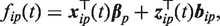
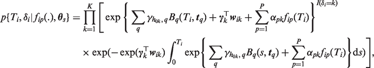
For the survival process we assume that the risk for each of the K competing events depends on the true but unobserved value of the markers at time t. Specifically, we have

h ik (t, θ s) = h 0 k (t) exp {γ_{k}^{⊤} w ik + \sum_{p = 1}^{P} α pk f ip (t)}, t > 0,

where θ_s is the parameter vector for the survival outcomes,

w ik

is a vector of baseline covariates with a corresponding vector of regression coefficients

γ k

, and α_pk denotes the strength of association between the longitudinal and survival outcomes. A B-splines baseline hazard function is assumed

log h 0 k (t) = γ h 0, 0 + \sum_{q = 1}^{Q} γ h 0, q B q (t, ν)

, where

B q (t, ν)

denotes the q-th basis function of a B-spline with knots

ν 1, \dots, ν Q

and

γ h 0

, the vector of spline coefficients. We place the knots at equally spaced percentiles of the observed event times.

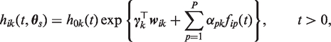
An issue that is often overlooked when building joint models is the functional form that describes the longitudinal outcomes that are associated with the risk for each event. Due to the fact that different structures may provide us with different inferences and predictions, it is important to study this component of the model. Following, Brown,¹⁴ Rizopoulos and Ghosh,¹⁵ and Rizopoulos,⁹ we postulate different functional forms to assess the predictive ability of the biomarkers. Specifically, we assume the following association structures:

M 1 : h ik (t, θ s) = h 0 k (t) exp {γ_{k}^{⊤} w ik + \sum_{p = 1}^{P} α pk f ip (t)}, M 2 : h ik (t, θ s) = h 0 k (t) exp {γ_{k}^{⊤} w ik + \sum_{p = 1}^{P} α pk f ip (t) + \sum_{p = 1}^{P} α_{pk}^{d} f' ip (t)} M 3 : h ik (t, θ s) = h 0 k (t) exp {γ_{k}^{⊤} w ik + \sum_{p = 1}^{P} α_{pk}^{d} \int_{0}^{t} f ip (s) d s},,

(1)

where

f_{ip}^{'} (t) = \frac{df ip (t)}{dt}

is the first order derivative of the

f ip (t)

function.

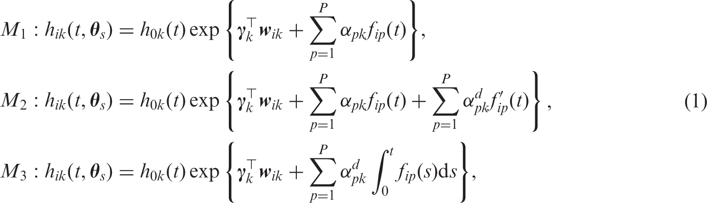
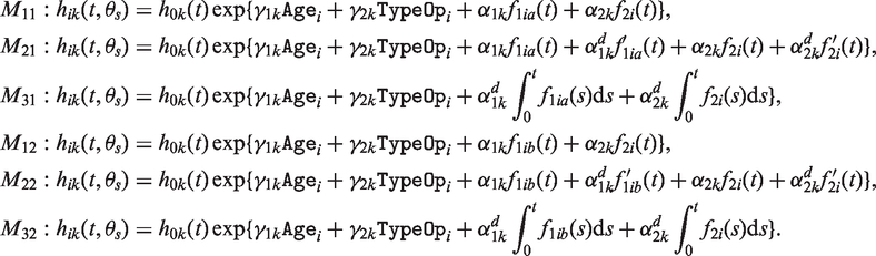
Model M₁ postulates that the risk for an event at time t depends on the mean level of the markers at the same time point t. Model M₂ is an extension of model M₁ in which not only the current value but also the slopes of the longitudinal trajectories at time t are related to the hazard. Yet another option is to relate the survival outcomes with a summary of the whole history of the markers, e.g. the area under the longitudinal profiles (model M₃).

Combinations of these parameterizations are possible, where in the case of 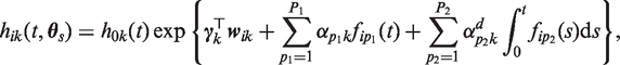$P = P 1 + P 2$ longitudinal outcomes we could have:

h ik (t, θ s) = h 0 k (t) exp {γ_{k}^{⊤} w ik + \sum_{p 1 = 1}^{P 1} α p 1 k f ip 1 (t) + \sum_{p 2 = 1}^{P 2} α_{p 2 k}^{d} \int_{0}^{t} f ip 2 (s) d s},

where the risk for an event at time t is associated with the underlying value of P₁ biomarkers at a specific time point and the area under the curve for P₂ biomarkers. Furthermore, different structures could be assumed for each survival model. A wide range of combined models will improve the efficiency of BMA and therefore more accurate predictions will be provided.

2.2 Bayesian estimation and prior specification

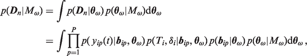
For the estimation of our joint model’s parameters, we adopt a Bayesian formulation and derive posterior inferences using a Markov Chain Monte Carlo (MCMC) algorithm. The likelihood of the model is derived under the assumption that the random effects account for all independencies between the observed outcomes. Specifically, given the random effects, the longitudinal and survival processes are assumed independent and moreover, the longitudinal responses of each subject are assumed independent. In particular,

p (y i, T i, δ i | b i; θ) = Π_{p = 1}^{P} p (y ip | b ip, θ y p) p {T i, δ i | f ip (.), θ s}, p (y ip | b ip; θ y p) = Π_{j = 1}^{n ip} p (y ipj | b ip; θ y p),

(2)

where

θ = (θ_{y p}^{⊤}, θ_{s}^{⊤}) ⊤

denotes the parameter vector for the longitudinal and survival outcomes. Thus, the posterior distribution is written as

p (θ | y ip, T i, δ i) \propto Π_{p = 1}^{P} Π_{j = 1}^{n ip} p (y ipj | b ip, θ y p) p {T i, δ i | f ip (.), θ s} p (b ip | θ y p) p (θ y p) p (θ s) .

The likelihood contribution from the exponential family takes the form

p (y ip | b ip, θ y p) = exp {\sum_{j = 1}^{n ip} [y ipj ψ ipj (b ip) - c {ψ ipj (b ip)} / a (φ) - d (y ipj, φ)]},

where

ψ ipj (b ip)

and φ denote the natural and dispersion parameters in the exponential family, respectively, and

c (.), d (.)

, and

a (.)

are known functions specifying the member of the exponential family. The likelihood contribution of the survival model when assuming the parametrization of model (1) is given by

p {T i, δ i | f ip (.), θ s} = Π_{k = 1}^{K} [exp {\sum_{q} γ h 0 k, q B q (T i, t q) + γ_{k}^{⊤} w ik + \sum_{p = 1}^{P} α pk f ip (T i)} I (δ i = k) \times exp (- exp (γ_{k}^{⊤} w ik) \int_{0}^{T i} exp {\sum_{q} γ h 0 k, q B q (s, t q) + \sum_{p = 1}^{P} α pk f ip (T i)} d s)],

The integral in the definition of the survival function does not have a closed-form solution, and therefore we used a 15-point Gauss–Kronrod quadrature rule to approximate it.¹⁶

We use standard prior distributions for the parameters. In particular, for the regression coefficients $β p$ , the survival coefficients $γ k$ , the association coefficients α_pk, and the baseline hazards for the survival submodel $γ h 0 k, q$ , normal priors are taken with mean 0 and variance 100. For the variance–covariance matrix D of the random effects we take inverse Wishart prior with an identity scale matrix and six degrees of freedom which is equal to the number of the random effects. Finally, for variance parameters (e.g. for normal longitudinal outcomes) inverse gamma priors are taken with parameters that are based on the separate analysis per outcome. In particular, we use the parameters $(1 / σ 2) 2 / 10$ and $(1 / σ 2) / 10$ , where $σ 2$ is the variance of the error term when fitting a mixed-effects model. These values are taken from the default arguments of the jointModelBayes function in the R package JMbayes.

All computations have been performed in R (version 3.1.2) and JAGS (version 3.3.0) and are available upon request from the first author.

3. Dynamic predictions of cumulative incidence functions

3.1 Predictions from a single model

Based on the joint models presented in Section 2.1, we focus on the derivation of the predictions of the survival outcomes. More specifically, we would like to predict cumulative incidence probabilities for a new patient l that has provided us with a set of longitudinal measurements $\tilde{Y} lp (t) = {y lp (s p 1), \dots, y lp (s pnl); 0 \leq s p 1 < s p 2 < \dots < s pnl < t, p = 1, \dots, P}$ . Given that no event occurred up to t, it is more relevant to focus on the cumulative incidence probabilities at time u > t. To account for competing risks we work with the cumulative incidence function

π lk (u, t) = P (T_{lk}^{*} < u | \cup_{k = 1}^{K} T_{lk}^{*} > t, \tilde{Y} l 1 (t), \dots, \tilde{Y} lP (t), D n),

where

D n = {T i, δ i, y i 1, \dots, y iP; i = 1, \dots, n}

denotes the sample on which the joint model was fitted.

Under the Bayesian formulation of the joint model, the estimation of $π lk (u, t)$ is based on the corresponding posterior predictive distributions, namely

π lk (u, t) = \int P (T_{lk}^{*} < u | \cup_{k = 1}^{K} T_{lk}^{*} > t, \tilde{Y} l 1 (t), \dots, \tilde{Y} lP (t); θ) p (θ | D n) d θ .

(3)

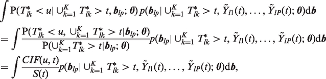
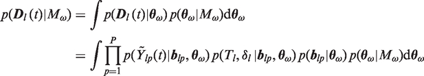
The second term of the integrant (3), 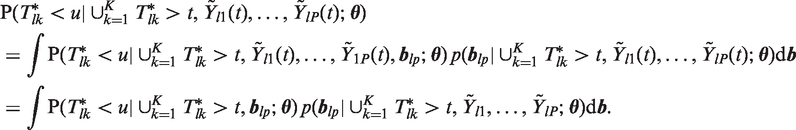$p (θ | D n)$ , is the posterior distribution of the parameters given the observed data. Using the full conditional independence assumption (2), the first term of the integrand in (3) can be written as (this can be seen in the last transition)

P (T_{lk}^{*} < u | \cup_{k = 1}^{K} T_{lk}^{*} > t, \tilde{Y} l 1 (t), \dots, \tilde{Y} lP (t); θ) = \int P (T_{lk}^{*} < u | \cup_{k = 1}^{K} T_{lk}^{*} > t, \tilde{Y} l 1 (t), \dots, \tilde{Y} 1 P (t), b lp; θ) p (b lp | \cup_{k = 1}^{K} T_{lk}^{*} > t, \tilde{Y} l 1 (t), \dots, \tilde{Y} lP (t); θ) d b = \int P (T_{lk}^{*} < u | \cup_{k = 1}^{K} T_{lk}^{*} > t, b lp; θ) p (b lp | \cup_{k = 1}^{K} T_{lk}^{*} > t, \tilde{Y} l 1, \dots, \tilde{Y} lP; θ) d b .

Furthermore, we have that

\int P (T_{lk}^{*} < u | \cup_{k = 1}^{K} T_{lk}^{*} > t, b lp; θ) p (b lp | \cup_{k = 1}^{K} T_{lk}^{*} > t, \tilde{Y} l 1 (t), \dots, \tilde{Y} lP (t); θ) d b = \int \frac{P (T_{lk}^{*} < u, \cup_{k = 1}^{K} T_{lk}^{*} > t | b lp; θ)}{P (\cup_{k = 1}^{K} T_{lk}^{*} > t | b lp; θ)} p (b lp | \cup_{k = 1}^{K} T_{lk}^{*} > t, \tilde{Y} l 1 (t), \dots, \tilde{Y} lP (t); θ) d b = \int \frac{CIF (u, t)}{S (t)} p (b lp | \cup_{k = 1}^{K} T_{lk}^{*} > t, \tilde{Y} l 1 (t), \dots, \tilde{Y} lP (t); θ) d b,

where

S (.)

denotes the overall survival and

CIF (.) = \int_{t}^{u} h lk (s) S (s) ds

the cumulative incidence function.

An estimate of $π lk (u, t)$ can be obtained using the following Monte Carlo simulation scheme:

1. Draw $θ *$ from the MCMC sample of the posterior $p (θ | D n)$

2. Draw $b_{lp}^{*}$ from $p (b lp | \cup_{k = 1}^{K} T_{lk}^{*} > t, \tilde{Y} l 1 (t), \dots, \tilde{Y} lP (t); θ *)$

3. Compute $π lk (u, t, b_{lp}^{*}; θ *) = CIF (u, t, b_{lp}^{*}; θ *) / S (t, b_{lp}^{*}; θ *)$

We, then, repeat steps 1–3 H times and derive the estimates of the 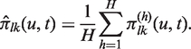$π lk (u, t)$ as,

\hat{π} lk (u, t) = \frac{1}{H} \sum_{h = 1}^{H} π_{lk}^{(h)} (u, t) .

Moreover, a 95% credible interval can be obtained using the Monte Carlo sample percentiles.

3.2 Combined predictions using BMA

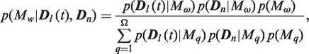
As it was seen in Section 2.1, there are several ways to link the longitudinal and the survival outcomes. Moreover, we could even postulate additional joint models with different assumptions for each submodel. For instance, in some of the mixed models the subject-specific evolutions over time may be non-linear, or we could control for different sets of baseline covariates either in the mixed-effects or relative-risk submodels. In this complex setting, a common practice is to choose a single model based on information criteria and obtain predictions from that selected model. However, this approach ignores model uncertainty. In addition, there may be different models that provide more accurate predictions for different types of subjects. An alternative solution to this problem is BMA, which proceeds by estimating a number of models and constructing a weighted average of predictions.^11,12

More formally, following the notation in Section 3.1, we would like to obtain predictions of the conditional probabilities 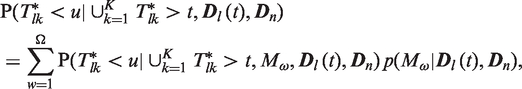$π lk (u, t)$ , u > t, for a new patient l who has provided us with a set of longitudinal outcomes $\tilde{Y} lp (t) = {y lp (s p 1), \dots, y lp (s pnl); 0 \leq s p 1 < s p 2 < \dots < s pnl < t, p = 1, \dots, P}$ . Assuming models $M 1, \dots, M Ω$ , the averaged conditional cumulative probabilities of patient l occurring an event at time u, given that he did not have any event up to time t is given by:

P (T_{lk}^{*} < u | \cup_{k = 1}^{K} T_{lk}^{*} > t, D l (t), D n) = \sum_{w = 1}^{Ω} P (T_{lk}^{*} < u | \cup_{k = 1}^{K} T_{lk}^{*} > t, M ω, D l (t), D n) p (M ω | D l (t), D n),

where

D n = {T i, δ i, y i 1, \dots, y iP; i = 1, \dots, n}

denotes the sample on which the joint models were fitted and

D l (t) = {\tilde{Y} lp (t), \cup_{k = 1}^{K} T_{lk}^{*} > t}

denotes the data of the new patient l. The first term of the above equation denotes the conditional cumulative probabilities per model and the second term denotes the posterior weights of each of the models. To calculate the posterior probability of the models we use Bayes rule as

p (M w | D l (t), D n) = \frac{p (D l (t) | M ω) p (D n | M ω) p (M ω)}{\sum_{q = 1}^{Ω} p (D l (t) | M q) p (D n | M q) p (M q)},

where

p (D l (t) | M ω) = \int p (D l (t) | θ ω) p (θ ω | M ω) d θ ω = \int Π_{p = 1}^{P} p (\tilde{Y} lp (t) | b lp, θ ω) p (T l, δ l | b lp, θ ω) p (b lp | θ ω) p (θ ω | M ω) d θ ω

and

p (D n | M ω) = \int p (D n | θ ω) p (θ ω | M ω) d θ ω = \int Π_{p = 1}^{P} p (y ip (t) | b ip, θ ω) p (T i, δ i | b ip, θ ω) p (b ip | θ ω) p (θ ω | M ω) d θ ω,

where

p (D l (t) | θ ω)

and

p (D n | θ ω)

are the likelihood functions for the new patient and for all patients in the study, respectively. Furthermore,

p (θ ω | M ω)

is the prior density of

θ ω

under model

M ω

. We obtain

p (D l (t) | M ω)

and

p (D n | M ω)

by means of Laplace approximations. Specifically, we first integrate out the random effects and then the parameters. A priori we assume that all models are equally probable. A careful investigation of

p (M ω | D l (t), D n)

reveals that different patients, but also different time points within the same patient, could provide different weights. Thus, compared to the choice of a single model, the BMA provides predictions that are more accurate since for every patient and visit it uses the models that are more probable to describe the association between the longitudinal and survival outcomes.

4. Analysis of the valve dataset

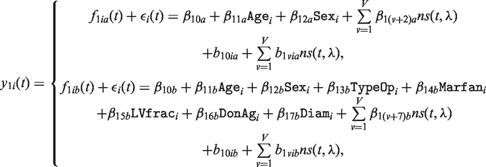
In this section we present the analysis of the cardio data introduced in Section 1. Our interest is to derive subject-specific risk predictions using all available information for a patient. We first started our analysis by fitting a set of joint models with different association structures and different baseline covariates. More specifically, for the linear mixed-effects model many patients showed non-linear longitudinal trajectories and therefore, we assumed natural cubic spline for time with two internal knots (λ) at 2.1 and 5.5 year (corresponding to 33.3% and 66.7% of the observed follow-up times) in both fixed and random part in the mixed-effects model of aortic gradient. Furthermore, we corrected for age (after we standardized it) and gender. Since there are more clinically relevant baseline covariates that have an effect on aortic gradient, we fitted a second mixed-effects model including also: marfan, left ventricular function, standardized donor age, and standardized diameter of valve. Particularly, the linear mixed-effects models take the form

y 1 i (t) = {f 1 ia (t) + ε i (t) = β 10 a + β 11 a Age i + β 12 a Sex i + \sum_{v = 1}^{V} β 1 (v + 2) a ns (t, λ) + b 10 ia + \sum_{v = 1}^{V} b 1 via ns (t, λ), f 1 ib (t) + ε i (t) = β 10 b + β 11 b Age i + β 12 b Sex i + β 13 b TypeOp i + β 14 b Marfan i + β 15 b LVfrac i + β 16 b DonAg i + β 17 b Diam i + \sum_{v = 1}^{V} β 1 (v + 7) b ns (t, λ) + b 10 ib + \sum_{v = 1}^{V} b 1 vib ns (t, λ),

where

ns (t, λ)

denotes the natural cubic spline matrix with two internal knots. For the CR mixed-effects model of aortic regurgitation we assumed linear time at the fixed part and a random intercept and slope at the random part. Finally, we corrected for age (after we standardized it) and gender. The CR mixed-effects model after the transformation of the ordinal outcome takes the form

P (y_{2 i}^{*} (t) = 1 | y 2 i * (t) \leq 1, Age, Sex, t, b 20, b 21) = \frac{exp {f 2 i (t)}}{1 + exp {f 2 i (t)}} = \frac{exp (\sum_{s = 0}^{4} β 2 s + β 25 Age i + β 26 Sex i + β 27 t + b 20 i + b 21 i t)}{1 + exp (\sum_{s = 0}^{4} β 2 s + β 25 Age i + β 26 Sex i + β 27 t + b 20 i + b 21 i t)} .

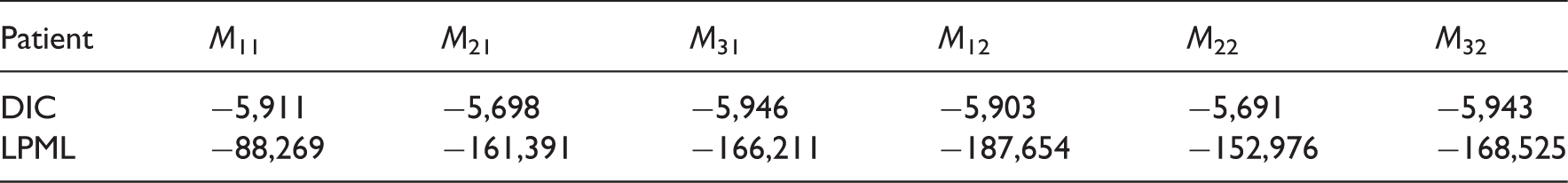
For the survival models we used proportional hazards models expressing the baseline hazard function with a B-splines function as described in Section 2.1. Standardized age and type of operation are important clinical factors and thus were included as confounders. Moreover, to not further complicate the analysis we assumed the same functional form for all longitudinal outcomes and the same model for all survival outcomes. Specifically, the joint models that we fitted take the form

M 11 : h ik (t, θ s) = h 0 k (t) exp {γ 1 k Age i + γ 2 k TypeOp i + α 1 k f 1 ia (t) + α 2 k f 2 i (t)}, M 21 : h ik (t, θ s) = h 0 k (t) exp {γ 1 k Age i + γ 2 k TypeOp i + α 1 k f 1 ia (t) + α_{1 k}^{d} f 1 ia' (t) + α 2 k f 2 i (t) + α_{2 k}^{d} f 2 i' (t)}, M 31 : h ik (t, θ s) = h 0 k (t) exp {γ 1 k Age i + γ 2 k TypeOp i + α_{1 k}^{d} \int_{0}^{t} f 1 ia (s) d s + α_{2 k}^{d} \int_{0}^{t} f 2 i (s) d s}, M 12 : h ik (t, θ s) = h 0 k (t) exp {γ 1 k Age i + γ 2 k TypeOp i + α 1 k f 1 ib (t) + α 2 k f 2 i (t)}, M 22 : h ik (t, θ s) = h 0 k (t) exp {γ 1 k Age i + γ 2 k TypeOp i + α 1 k f 1 ib (t) + α_{1 k}^{d} f 1 ib' (t) + α 2 k f 2 i (t) + α_{2 k}^{d} f 2 i' (t)}, M 32 : h ik (t, θ s) = h 0 k (t) exp {γ 1 k Age i + γ 2 k TypeOp i + α_{1 k}^{d} \int_{0}^{t} f 1 ib (s) d s + α_{2 k}^{d} \int_{0}^{t} f 2 i (s) d s} .

We run the MCMC with single chains for 550,000 iterations for all models and we discarded 50,000 iterations as burn-in. Convergence was monitored by trace plots and the Geweke diagnostic test. Tables 1–6 in the Supplementary material in Section 1 (available at: http://smm.sagepub.com/) shows the posterior means, standard errors, and corresponding 95% credible intervals for the parameters of the longitudinal and survival submodels, respectively. As it can be seen, age is significantly associated with death in all models and with reoperation in models M₁₁, M₁₂, M₃₁, and M₃₂ where the survival outcomes are associated with the true value and the area under the curve of the biomarkers. Moreover, type of operation seems to be a significant factor for death in models M₁₁ and M₁₂. Furthermore, the underlying value, the slope, and the area under the curve of aortic gradient seem to be associated with death in both set of joint models with the less and extra baseline covariates in the mixed-effects model while only M₂₁ showed a non significant association of the underlying value with reoperation. From models M₁₁, M₁₂, M₂₁, and M₂₂ we obtain that the underlying value of aortic regurgitation is a significant factor for death and reoperation. In addition, we used the deviance information criterion (DIC) and the log pseudo-marginal likelihood (LPML) to measure the models’ predictive ability.¹⁷ The choice of these measures instead of other traditional measures, such as the Brier score and the area under the ROC curve, is motivated by the fact that no established accepted extension of the latter measures exists in the context of competing risks. Specifically, from Table 2 models M₃₁ and M₃₂ appear to provide a better fit to the data according to the DIC which is based on a penalized deviance approach and model M₁₁ according to LPML which is based on a cross-validated approach. The results of the DIC and LPML seem to be different, therefore, further investigation was performed. In particular, in the supplementary material in Figure 1, we present the conditional predictive ordinate of 12 randomly selected patients. As it is shown, different patients have different best model and even two models performing almost the same. It is evident that an approach, such as the BMA, would be more flexible since it uses all available models instead of choosing a single one. More details about the DIC, the conditional predictive ordinate, and LPML are presented in the supplementary material in Section 2.

Table 2.

DIC and LPML measurements for the six joint models.

Patient	M ₁₁	M ₂₁	M ₃₁	M ₁₂	M ₂₂	M ₃₂
DIC	−5,911	−5,698	−5,946	−5,903	−5,691	−5,943
LPML	−88,269	−161,391	−166,211	−187,654	−152,976	−168,525

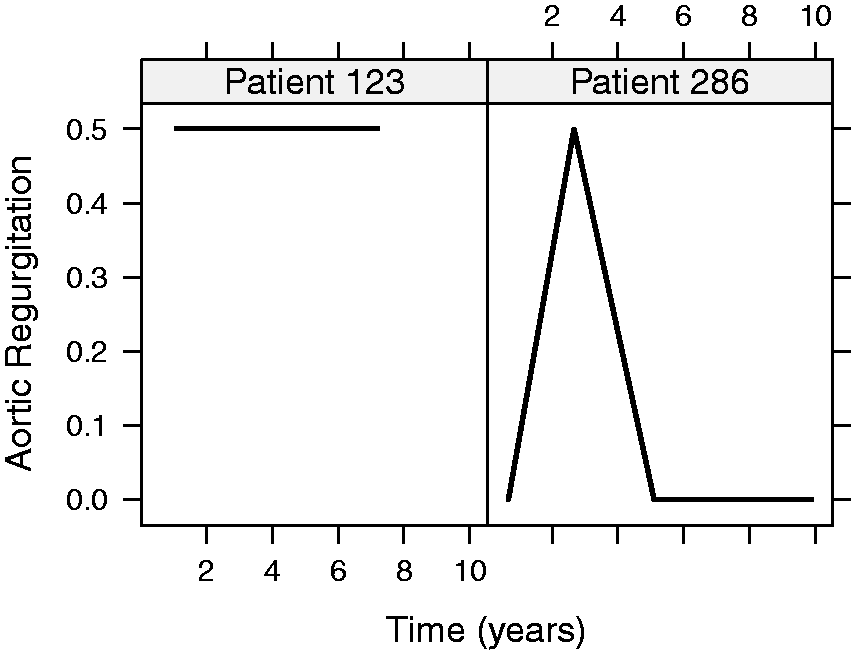
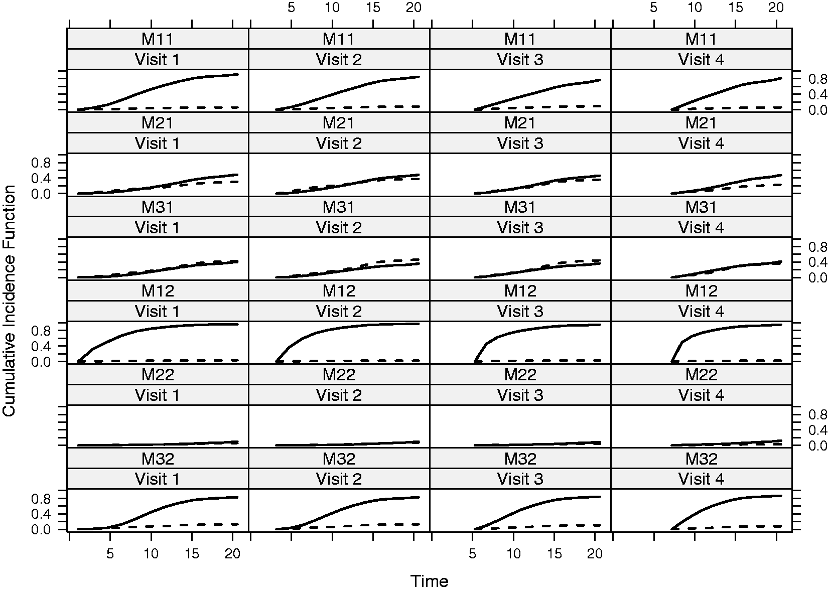
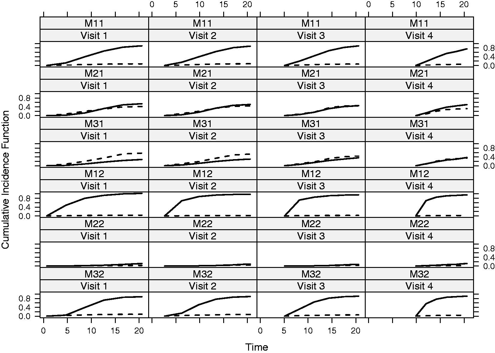
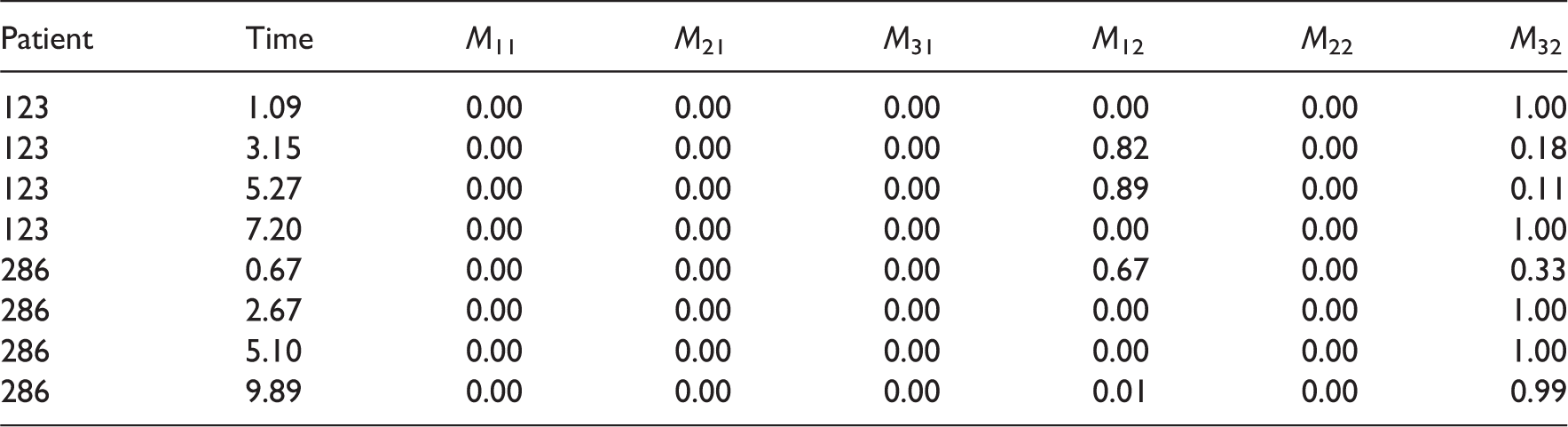
We continued by calculating dynamic predictions based on the models described above. Under the fitted joint models, the conditional probabilities of death and reoperation were estimated using the Monte Carlo procedure, as described in Section 3.1, with H = 300. Specifically, we derived the predictions of two patients, patient 123 (47-year-old male) and patient 286 (52-year-old male), that were excluded from the dataset when fitting the joint models. In Figures 2 and 3, we present the longitudinal trajectories of these patients, which are also highlighted in Figure 1. As it can be seen, both patients show an increasing aortic gradient profile over time, but, patient 286 has higher values than patient 123. For aortic regurgitation, only patient 286 seems to change category at the second follow-up. We show the predictions of every joint model of death and reoperation for patients 123 and 286 in Figures 4 and 5, as more longitudinal measurements are available. For patient 123, when using the underlying value of aortic gradient and aortic regurgitation in the survival models (for both the model with less M₁₁ and more covariates M₁₂ as confounder in the longitudinal part), the conditional probabilities of death are much smaller than reoperation. The same can be seen when assuming the area under the curve model with the extra confounder M₃₂. However, when assuming the slope parameterization and the area under the curve parameterization (for the model without the extra clinical relevant covariates), the difference between the survival and free intervention probabilities is smaller (M₂₁, M₂₂, and M₃₁). Specifically, the probabilities of death and reoperation seem to cross in model M₂₁ while, in model M₂₂ both are really small. For patient 286, a bigger difference between the death and survival probabilities is observed in model M₃₁ compared to patient 123. Furthermore, in model M₂₁ it is clear that the probability of death is higher in the next five years at the first two visits.

Figure 2.

Profile plots of aortic gradient for patients 123 and 286.

Figure 3.

Profile plots of aortic regurgitation for patients 123 and 286.

Figure 4.

Prediction plots for patient 123 using each joint model proposed. Solid line represents the reoperation predictions and dashed line the death predictions.

Figure 5.

Prediction plots for patient 286 using each joint model proposed. Solid line represents the reoperation predictions and dashed line the death predictions.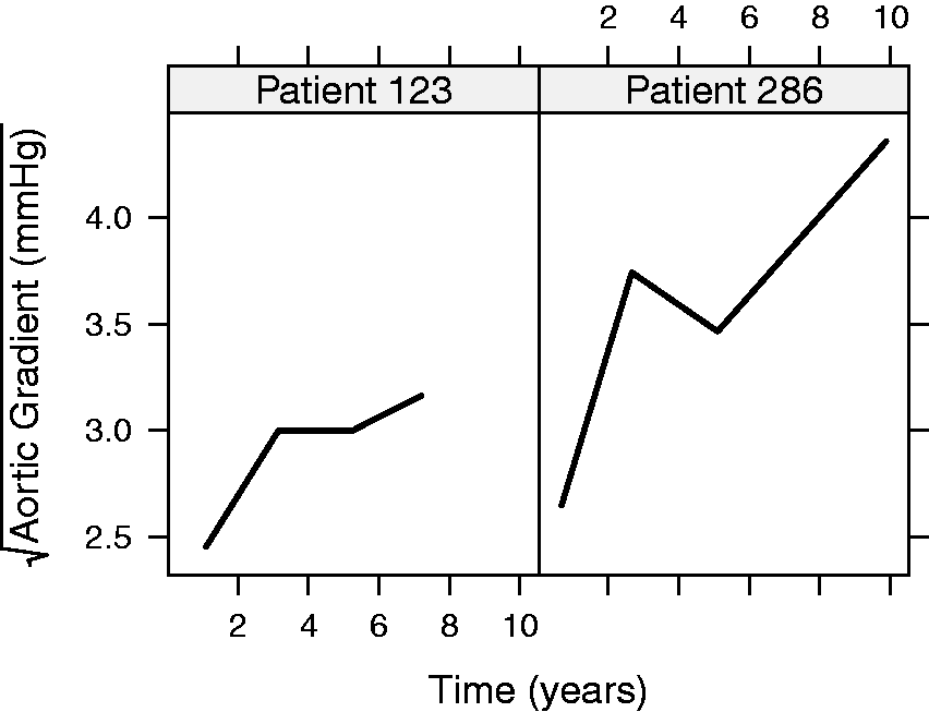

Following, we computed the posterior weight for each model and calculated the BMA predictions. In Table 3, we present the weights of the models for each patient and visit. It is clear that not always a single model provides the best prediction. Specifically, models M₁₂ and M₃₂ seem to contribute in the BMA predictions depending on the patient and the visit. As it can be seen, even within the same patient the choice of the best model could change over time. In particular, for patient 123 at the first and last visit we observe that only model M₃₂ provides better predictions. However, for the second and third visit we obtain a higher contribution for model M₁₂. This could be explained by the fact that the square root of aortic gradient of the specific patient remains the same for visits 2 and 3, thus the whole profile of the patient is not needed. Furthermore, for patient 286 we obtain that model M₁₂ contributes 67% and model M₃₂ 33% at the calculation of the predictions at visit one. After the first visit, M₃₂ is chosen to be the most appropriate model. From the profile plots, we obtain a decrease of the square root aortic gradient from visit 2 to visit 3 and an increased aortic regurgitation at visit 2, therefore the whole evolution of the outcome may be a better predictor after the second visit. In Figures 6 and 7, which present the combined predictions, we obtain high probabilities for reoperation and low for death for both patients (credible intervals for reoperation and death for patient 123 are presented in the supplementary material in Figures 2 and 3, respectively). This is explained by the fact that both models M₁₂ and M₃₂ indicate the same behavior. In the supplementary material, in Figures 6 to 9 we present also predictions for individual 281 who is a 16-year-old female patient with profile plots of aortic gradient and aortic regurgitation that are presented in the supplementary material in Figures 4 and 5 (aortic gradient measurements are also highlighted in Figure 1). As we can see there is a bigger difference between the conditional probabilities of death and reoperation compared to the male patients.

Table 3.

Bayesian model averaging posterior weights for the six proposed joint models for patient 123 and 286 for each measurement.

Patient	Time	M ₁₂	M ₃₂
123	1.09	0.00	1.00
123	3.15	0.82	0.18
123	5.27	0.89	0.11
123	7.20	0.00	1.00
286	0.67	0.67	0.33
286	2.67	0.00	1.00
286	5.10	0.00	1.00
286	9.89	0.01	0.99

Figure 6.

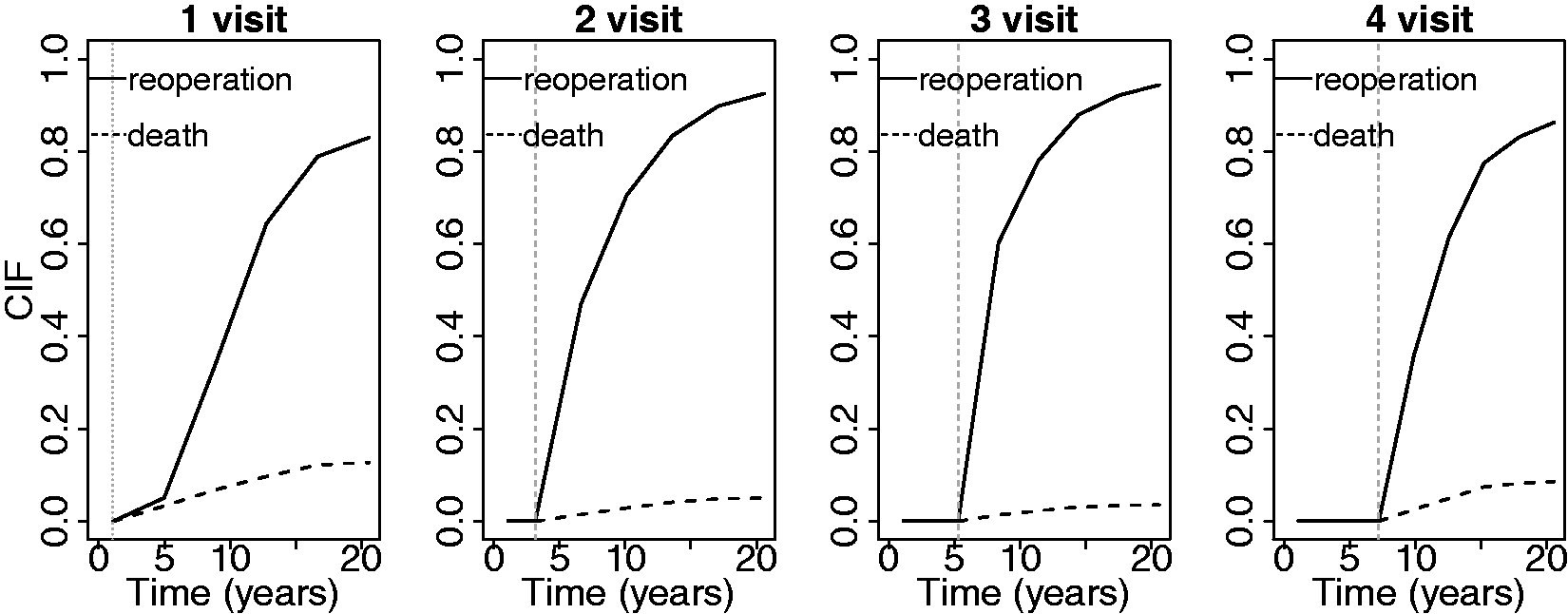
Prediction plots for patient 123 using Bayesian model averaging - CIF = Cumulative Incidence Function.

Figure 7.

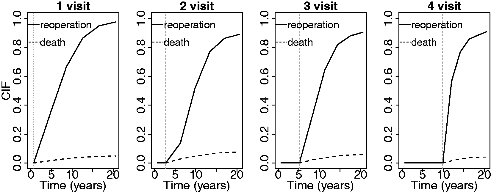
Prediction plots for patient 286 using Bayesian model averaging - CIF = Cumulative Incidence Function.

5. Simulation

We performed a simulation study in order to evaluate the performance of the proposed approach. Simulations showing that BMA predictions perform well in comparison with predictions from the true model have been already presented in the literature.¹² Therefore, in this paper we focus on the comparison between the BMA with the DIC approach in a setting where patients are simulated from different scenarios. As mentioned before, it is common practice that a single model is selected using standard criteria, such as DIC, and then, for every new patient predictions are based on this specific model. However, this raises the question whether it is appropriate to assume the same prediction model for patients with different features in their longitudinal profile.

Motivated by this, we simulated 200 datasets that consist of 140 subjects per scenario. In particular, we considered three scenarios corresponding to the three parameterizations: (1) value, (2) slope, and (3) area. Under each scenario and for each simulated dataset, we randomly selected 20 subjects and calculated the BMA weights. Since patients within a dataset could have different characteristics, we merged the remaining subjects and fitted the three joint models assuming the parameterizations (1), (2), (3) in order to obtain the DIC values. For simplicity we assumed one longitudinal and one survival outcome. A detailed description of the design of this simulation study is presented in the supplementary material in Section 3. In Figure 8 we show on the X-axis the models selected by the DIC approach and on the Y-axis the mean weights of the not selected from the DIC models obtained from the BMA approach. Assuming that the DIC selects the appropriate model and assuming that the BMA has a similar behavior, we would expect a value close to 0 for the weights. In the opposite case where the approaches are not consistent we would expect the weights to be higher than zero depending on the degree of disagreement, where one indicates a strong disagreement. As can be seen, when the value model is selected by DIC, the mean weights of the other models (slope and area) are mostly between 0.6 and 0.85, whereas in the case where the area model is selected by the DIC, these are close to 1.

Figure 8.

Mean weights for the models that were not selected by the DIC.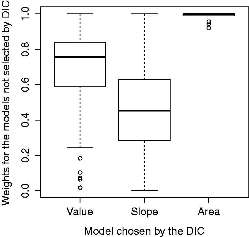

6. Discussion

Time-dependent adjustment of risk prediction models for patients with severe heart valve diseases, as more longitudinal measurements become available over time, provides the physician with an evidence-based understanding of the prognostic implication of changes in the patient’s disease condition. Importantly, the calculated probabilities for survival and re-intervention can be used as an early warning system, allowing the necessary time for the physicians to plan an intervention. In this work we presented dynamic predictions for a competing risk setting using multiple longitudinal outcomes. Specifically, we performed different functional forms to relate the longitudinal and the survival processes and different structure (by adding clinical relevant baseline covariates) of one longitudinal model and investigate the predictions of two patients that we originally excluded from the dataset. Finally, since the choice of a single model ignores the model uncertainty issue, we combined all models and derived predictions for the survival outcomes for the same two patients using the BMA. This method explicitly accounts for model uncertainty and for the fact that not all future patients have the same prognostic model. Despite the usefulness of the BMA approach, there are some issues that we need to be caution for. In particular, the specification of the prior distribution of the models is challenging and has received little attention. Moreover, the number of models that could be combined may be high resulting to difficulties in calculating the summation. We should, furthermore, make clear that we cannot identify the true model from the pool of all candidate models.

An alternative measure to the survival time is the cause-specific residual life that provides the expected value for the lifetime remaining at any time t, given that the subject is known to have survived up to t.¹⁸ The advantage of the residual life function over the survival function lies in its interpretation in many applications where the primary aim is to characterize the remaining time expectancy of a subject instead of the failure rate. For instance, patients may wish to learn from their physicians an estimate of their expected survival given that they have started a treatment or received an intervention at a given time. This idea is similar to the conditional cumulative incidence functions for death and reoperation that we presented in the paper, where death and reoperation probabilities are calculated at time u given that the patient did not experience any event at t, t < u.

We limited our work so that the association between aortic gradient and aortic regurgitation with the survival outcomes was the same. However, a different functional form for each biomarker would be also possible and interesting to investigate. A disadvantage, nevertheless, is that it will be more computationally intensive, since more models would be fitted. Moreover, additional ways to link the longitudinal and survival processes, such as the weighted area under the curve, the lag effect, and the shared random effect parameterization, were not addressed in this paper. Nevertheless, a bigger dataset with patients followed for a longer period is probably needed in order to obtain a variety of evolutions and capture the special characteristics of the patients. Furthermore, we performed models including extra confounders only for the continuous longitudinal outcome. Hence, more factors in the model of the ordinal outcome and also of the survival outcomes could be included and further investigated. In this paper we did not perform any formal validation of the derived predictions. Measures for the evaluation of calibration and discrimination of prognostic survival models can be easily adapted to the competing risks setting.^19,20 Within the joint modeling framework, calibration and discrimination has been previously introduced.^4,5 However to our knowledge these proposed measures of calibration and discrimination are not directly applicable on competing risk settings. Thus, validation in that setting may be an interesting topic for future research. In addition, in the paper, for the calculation of the marginal densities $p (D n | M ω)$ and $p (D l (t) | M ω)$ in the BMA approach, we used the Laplace approximation. However, different approaches could be applied and further investigated. In general, the combination of a continuous and an ordinal longitudinal outcome was challenging. Specifically, the ordinal outcome aortic regurgitation that consists of five categories increases the computational time drastically. Furthermore, the predictions under the area parameterization models were also time-consuming. In particular, these time-consuming computations seem to appear in the integration of time in the calculation of the survival in the $\frac{CIF (u, t)}{S (t)}$ part. Therefore, in order to optimize the execution runtime, the specific integral could be replaced by an approximation such as a 15-point Gauss–Kronrod rule (which was also used for the likelihood of the survival).

Supplemental Material

sj-pdf-1-smm-10.1177_0962280215588340 - Supplemental material for Combined dynamic predictions using joint models of two longitudinal outcomes and competing risk data

Supplemental material, sj-pdf-1-smm-10.1177_0962280215588340 for Combined dynamic predictions using joint models of two longitudinal outcomes and competing risk data by Eleni-Rosalina Andrinopoulou, D Rizopoulos, Johanna JM Takkenberg, E Lesaffre, in Statistical Methods in Medical Research

Footnotes

Declaration of conflicting interests

The author(s) declared no potential conflicts of interest with respect to the research, authorship, and/or publication of this article.

Funding

The author(s) received no financial support for the research, authorship, and/or publication of this article.

References

Taylor

Sandler

. Individualized predictions of disease progression following radiation therapy for prostate cancer. J Clin Oncol 2005; 23: 816–825.

Garre

Zwinderman

Geskus

, et al. A joint latent class change point model to improve the prediction of time to graft failure. J R Stat Soc, Ser A 2008; 171: 299–308.

Taylor

Sandler

. Individualized prediction in prostate cancer studies using a joint longitudinal survival-cure model. J Am Stat Assoc 2008; 103: 178–187.

Proust-Lima

Taylor

. Development and validation of a dynamic prognostic tool for prostate cancer recurrence using repeated measures of posttreatment PSA: a joint modeling approach. Biostatistics 2009; 10: 535–549.

Rizopoulos

. Dynamic predictions and prospective accuracy in joint models for longitudinal and time-to-event data. Biometrics 2011; 67: 819–829.

Bekkers

Klieverik

Raap

, et al. Re-operations for aortic allograft root failure: experience from a 21-year single-center prospective follow-up study. Eur J Cardio-Thorac Surg 2011; 40: 35–42.

Wulfsohn

Tsiatis

. A joint model for survival and longitudinal data measured with error. Biometrics 1997; 53: 330–339.

Tsiatis

Davidian

. Joint modeling of longitudinal and time-to-event data: an overview. Statistica Sinica 2004; 14: 809–834.

Rizopoulos D. Joint models for longitudinal and time-to-event data with applications. Boca Raton: Chapman R and Hall/CRC Biostatistics Series, 2012.

10.

Andrinopoulou

Rizopoulos

Takkenberg

, et al. Joint modeling of two longitudinal outcomes and competing risk data. Stat Med 2014; 33: 3167–3178.

11.

Hoeting

Madigan

Raftery

, et al. Bayesian model averaging: a tutorial. Stat Sci 1999; 14: 382–417.

12.

Rizopoulos

Hatfield

Carlin

, et al. Combining dynamic predictions from joint models for longitudinal and time-to-event data using Bayesian model averaging. J Am Stat Assoc 2014; 109: 1385–1397.

13.

Harrell

. Regression modeling strategies: with applications to linear models, logistic regression, and survival analysis, New York: Springer-Verlag, 2001.

14.

Brown

. Assessing the association between trends in a biomarker and risk of event with an application in pediatric HIV/AIDS. Ann Appl Stat 2009; 3: 1163–1182.

15.

Rizopoulos

Ghosh

. A Bayesian semiparametric multivariate joint model for multiple longitudinal outcomes and a time-to-event. Stat Med 2011; 30: 1366–1380.

16.

Press

Teukolsky

Vetterling

, et al. Numerical recipes: the art of scientific computing, 3rd ed. New York: Cambridge University Press, 2007.

17.

Lesaffre

Lawson

. Bayesian biostatistics, New York: Wiley & Sons, 2012.

18.

Jeong

Fine

. A note on cause-specific residual life. Biometrika 2009; 96: 237–242.

19.

Gail

Pfeiffer

. On criteria for evaluating models of absolute risk. Biostatistics 2005; 6: 227–239.

20.

Schoop

Beyersmann

Schumacher

, et al. Quantifying the predictive accuracy of time-to-event models in the presence of competing risks. Biom J 2011; 53: 88–112.

Supplementary Material

Please find the following supplemental material available below.

For Open Access articles published under a Creative Commons License, all supplemental material carries the same license as the article it is associated with.

For non-Open Access articles published, all supplemental material carries a non-exclusive license, and permission requests for re-use of supplemental material or any part of supplemental material shall be sent directly to the copyright owner as specified in the copyright notice associated with the article.

0.00 MB

0.11 MB