Standardized likelihood ratio test for comparing several log-normal means and confidence interval for the common mean

Abstract

Standardized likelihood ratio test (SLRT) for testing the equality of means of several log-normal distributions is proposed. The properties of the SLRT and an available modified likelihood ratio test (MLRT) and a generalized variable (GV) test are evaluated by Monte Carlo simulation and compared. Evaluation studies indicate that the SLRT is accurate even for small samples, whereas the MLRT could be quite liberal for some parameter values, and the GV test is in general conservative and less powerful than the SLRT. Furthermore, a closed-form approximate confidence interval for the common mean of several log-normal distributions is developed using the method of variance estimate recovery, and compared with the generalized confidence interval with respect to coverage probabilities and precision. Simulation studies indicate that the proposed confidence interval is accurate and better than the generalized confidence interval in terms of coverage probabilities. The methods are illustrated using two examples.

Keywords

Constrained maximum likelihood estimates modified likelihood ratio test power method of variance estimate recovery third-order accurate type I error rates

1 Introduction

Log-normal distributions are routinely postulated in epidemiological and health related studies where skewed distributions are more common.^1–4 Especially in biomedical research, including gene expression, many researchers showed that such skewed distributions can be accurately modeled by log-normal distribution. For example, Lee⁵ showed that growth rates of soft tissue metastases of breast cancer can be modeled by log-normal distribution; Bengtsson et al.⁶ observed that the transcript levels of five different genes in individual cells from mouse pancreatic islets are log-normally distributed. Neti and Howell⁷ provided experimental evidence of log-normal distribution of cellular radioactivity within a cell population. The main difference between normal and log-normal distribution is that in log-normal distribution random effects are multiplicative while in normal distribution these effects are additive. A classical example of multiplicative random effects in biological mechanisms is the bacteria in exponential growth (Limpert et al.⁸), where the numbers of organisms in different colonies show log-normal distribution. It is therefore important to accurately model biological data to account for biological variability. In fact, problems with using the normal distribution instead of the log-normal in medicine and life sciences are well addressed in many articles; for example, see Heath⁹ and Sorrentino.¹⁰

Exposure variables in industrial hygiene and epidemiology such as workplace pollution and indoor radon gas concentrations are also commonly modeled by log-normal distributions. The mean of the log-normal distribution is used to assess the exposure level or pollution level in an environment, which necessitates estimation of a log-normal mean; see Rappaport and Selvin,¹¹ Selvin and Rappaport,¹² and Krishnamoorthy et al.¹³ Estimation of log-normal mean also arises to assess health care costs (Griswold et al.¹⁴) and in pharmacokinetics data analysis (Shen et al.¹⁵). Assuming log-normal distributions for hospital charges, Zhou et al.¹⁶ have proposed a likelihood ratio test (LRT) for comparing two log-normal means; similarly, Krishnamoorthy and Mathew¹⁷ have provided a generalized variable (GV) approach to compare the means of carbon monoxide emission levels at two different sites considering log-normal models. However, the problem of comparing several log-normal means has not received much attention in the literature even though such problems arise frequently, for example in medical diagnostic of diseases with similar symptoms. Available LRT is applicable only for large samples, and tests for small samples are really warranted. Our investigation of statistical methods for comparing means of several log-normal distributions, and estimating the common mean of several log-normal populations is motivated by the following examples.

1.1 An example for comparing several log-normal means

Retrospective data were collected (between January 1990 and December 2012) from 75 infants at Louisiana State University Health Sciences Center (LSUHSC) who were less than three months of age at the time of diagnosis with total anomalous pulmonary venous return (TAPVR) and underwent a repair surgery. The pulmonary veins are the four blood vessels that return oxygen-rich blood from the lungs to the left atrium of the heart. The TAPVR is a rare heart disease that is present at birth in which none of the four veins that take blood from the lungs to the heart is attached to the left atrium; instead all four pulmonary veins drain abnormally to the right atrium by way of an abnormal connection. Infants with obstructed TAPVR are usually critically ill immediately after birth and need emergency surgery to restore the normal blood flow from the pulmonary veins to the left atrium. TAPVR is classified into four different types, based on how and where the pulmonary veins drain to the heart: in the supracardiac type (SC), the pulmonary veins drain into the right atrium through the superior vena cava. In the cardiac type (C), the pulmonary veins can directly enter into the right side of the heart, into the right atrium, or alternatively the pulmonary veins can drain into the coronary sinus. In the infracardiac type (IC), the pulmonary veins drain into the right atrium through the liver veins and the inferior vena cava. In the mixed type (M), the pulmonary veins split up and drain partially to more than one of these options. The SC, C, IC and M occur approximately in 45%, 25%, 25%, 5% of patients with TAPVR, respectively (Hirsch and Bove¹⁸). Specific surgical repair depends on the type of anomalous connection, thus correct preoperative diagnosis and accurate description of the drainage sites (anatomy types) are extremely important. A statistical problem of interest here is to compare deep hypothermic circulatory arrest time (in minutes) of the four anatomical TAPVR subtypes among the patients who underwent surgical repair. The data on deep hypothermic circulatory arrest time for these 75 infants are given in Table 8. Among those 75 infants with TAPVR, 24 infants were in type SC, 10 were in type C, four were in type M, and 37 were in type IC. Probability plots (Minitab 14; not reported here) for these four data sets indicated log-normality assumption is tenable. The log-normal probability plot for the subtype M with four measurements indicates that the log-normality assumption is barely tenable (p value = .109), and so we will not include this group for comparison. The probability plot for the subtype M in prolonged cardiopulmonary bypass time (data in Table 9) indicates that the log-normality assumption is tenable (p value = .754). However, the test may not be accurate for such small samples. Nevertheless, we assume log-normality, because some biomedical data follow the log-normal distribution based on scientific justifications rather than statistical tests.

1.2 Common mean problem

Suppose that the null hypothesis of equality of log-normal means is rejected then some standard multiple comparison methods such as the Bonferroni can be used to find the means that are significantly different. On the other hand, if the null hypothesis of equality of log-normal means is not rejected, then it may be of interest to estimate the unknown common mean. As noted by Tian and Wu,¹⁹ there are situations where several log-normal populations may have the same mean, and the problem of interest is to estimate or to test the common mean. An example for estimating the common mean described in Tian and Wu¹⁹ is as follows. In the Alcohol Interaction Study in Men (Bradstreet and Liss²⁰), 23 healthy male subjects completed a five period crossover study. Each subject was assigned randomly to one of the five treatments, namely, no treatment (control) or one of four active treatments from the same drug class used to treat the same illness. A washout period of one week separated the treatment periods. If the maximum serum ethanol level (C_max) or the area under the serum ethanol curve (AUC) from four active treatments can be considered as log-normally distributed with common mean, it is of interest to make inference about the common mean of the four active treatments.

For comparing the means of several log-normal distributions, Gill²¹ has proposed a modified version of the likelihood ratio test (MLRT). However, this MLRT, as shown in the sequel, is not defined for all samples. In fact, for both data sets in the example sections, the MLRT is undefined; see Remark 1. As a consequence, the approximate Chi-square distribution of the MLRT is doubtful. Li²² has proposed a test based on the GV approach which is a special case of the fiducial approach. In general, the fiducial approach for a multiparameter case is not well explained. Fiducial distributions for multiparameter problems are not necessarily unique and it is often unclear how to proceed; see Section 2.6.5 of Welsh.²³ Furthermore, our simulation studies in the sequel indicate that the GV test could be very liberal or conservative, and its power could decrease with increasing disparity among the means.

Keeping the two problems described earlier in mind, we have organized the rest of the article as follows. In the following section, we describe the MLRT by Gill,²¹ the SLRT for equality of several log-normal means, and the GV test. For the two-sample case, we also describe the test based on the confidence interval (CI) given in Zou et al.²⁴ The tests are compared with respects to type I error rates and powers. In Section 3, we address the common mean problem, and outline two estimation methods, one is based on the method of variance estimates recovery (MOVER), and another is based on the GV approach. We also evaluated the estimation methods with respect to coverage probabilities and precision using Monte Carlo simulation. The new proposed methods for both problems are not only simple, but also (as indicated by our simulation studies) better than other existing methods. The methods are illustrated using the two examples described earlier. Some concluding remarks are given in Section 4.

2 Tests for equality of log-normal means

Let $Y_{i 1}, \dots, Y_{{in}_{i}}$ be a sample from a log-normal distribution with parameters μ_i and $σ_{i}^{2}, i = 1, \dots, k$ . The mean of the ith log-normal distribution is $exp (μ_{i} + . 5 σ_{i}^{2})$ , and the problem of interest is to test the equality of the means; that is, to test

H_{0} : exp (μ_{1} + . 5 σ_{1}^{2}) = \dots = exp (μ_{k} + . 5 σ_{k}^{2})

Let $X_{ij} = \ln (Y_{ij}), j = 1, \dots, n_{i}, i = 1, \dots, k$ . Noting that $X_{i 1}, \dots, X_{{in}_{i}}$ follow a $N (μ_{i}, σ_{i}^{2})$ distribution, the problem of testing above hypothesis simplifies to testing

H_{0} : η_{1} = \dots = η_{k} vs . H_{a} : η_{i} \neq η_{j} for some i \neq j

(1)

where

η_{i} = μ_{i} + . 5 σ_{i}^{2}, i = 1, \dots, k

, based on

{\bar{X}}_{i} = \frac{1}{n_{i}} \sum_{j = 1}^{n_{i}} X_{ij} and V_{i}^{2} = \frac{1}{n_{i}} \sum_{j = 1}^{n_{i}} (X_{ij} - {\bar{X}}_{i})^{2}, i = 1, \dots, k

(2)

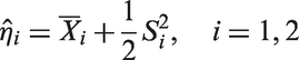
Note that ${\hat{μ}}_{i} = {\bar{X}}_{i}$ and ${\hat{σ}}_{i}^{2} = V_{i}^{2}$ are the maximum likelihood estimates (MLEs) of μ_i and $σ_{i}^{2}$ , respectively.

The log-likelihood function is given by

\ln L (μ_{1}, \dots, μ_{k}; σ_{1}^{2}, \dots, σ_{k}^{2}) = - \frac{1}{2} \sum_{i = 1}^{k} n_{i} \ln (σ_{i}^{2}) - \frac{1}{2} \sum_{i = 1}^{k} \frac{n_{i} V_{i}^{2} + n_{i} ({\bar{X}}_{i} - μ_{i})^{2}}{σ_{i}^{2}}

(3)

The log-likelihood function under $H_{0} : η_{1} = \dots = η_{k}$ can be expressed as

\ln L (η - . 5 σ_{1}^{2}, \dots, η - . 5 σ_{k}^{2}; σ_{1}^{2}, \dots, σ_{k}^{2}) = - \frac{1}{2} \sum_{i = 1}^{k} n_{i} \ln (σ_{i}^{2}) - \frac{1}{2} \sum_{i = 1}^{k} \frac{n_{i} V_{i}^{2} + n_{i} ({\bar{X}}_{i} - η + . 5 σ_{i}^{2})^{2}}{σ_{i}^{2}}

(4)

where η is the common unknown parameter under H₀ in equation (1). The values of

(η, σ_{1}^{2}, \dots, σ_{k}^{2})

that maximize equation (4) are the constrained MLEs, and let us denote the constrained MLEs by

({\hat{η}}_{c}, {\hat{σ}}_{1 c}^{2}, \dots, {\hat{σ}}_{kc}^{2})

As the test that we will propose in the sequel involves repeated calculation of the constrained MLEs, details for calculating the constrained MLEs and an algorithm are given in Appendix 1.

Recall that the usual MLE of μ_i is ${\hat{μ}}_{i} = {\bar{X}}_{i}$ and that of $σ_{i}^{2}$ is ${\hat{σ}}_{i}^{2} = V_{i}^{2}$ defined in equation (2). Then the LRT statistic is expressed as

Λ = 2 [\ln L ({\hat{μ}}_{1}, \dots, {\hat{μ}}_{k}; {\hat{σ}}_{1}^{2}, \dots, {\hat{σ}}_{k}^{2}) - \ln L ({\hat{η}}_{c} - . 5 {\hat{σ}}_{1 c}^{2}, \dots, {\hat{η}}_{c} - . 5 {\hat{σ}}_{kc}^{2}; {\hat{σ}}_{1 c}^{2}, \dots, {\hat{σ}}_{kc}^{2})]

= \sum_{i = 1}^{k} \frac{n_{i}}{{\hat{σ}}_{ic}^{2}} [V_{i}^{2} + ({\bar{X}}_{i} + . 5 {\hat{σ}}_{ic}^{2} - {\hat{η}}_{c})^{2}] - \sum_{i = 1}^{k} n_{i} \ln (\frac{{\hat{σ}}_{i}^{2}}{{\hat{σ}}_{ic}^{2}}) - \sum_{i = 1}^{k} n_{i}

(5)

For a given level of significance α, the LRT rejects the null hypothesis when $Λ > χ_{k - 1; 1 - α}^{2}$ , where $χ_{m; q}^{2}$ denotes the 100q percentile of the Chi-square distribution with df = m.

2.1 The modified likelihood ratio test

Following the general approach of Skovgaard,²⁵ Gill²¹ has proposed the following correction to the LRT statistic Λ in equation (5). To describe this test, let

θ = (μ_{1} / σ_{1}^{2}, \dots, μ_{k} / σ_{k}^{2}, 1 / σ_{1}^{2}, \dots, 1 / σ_{k}^{2})'

τ = (μ_{1}, \dots, μ_{k}, - . 5 n_{1} (μ_{1}^{2} + σ_{1}^{2}), \dots, - . 5 n_{k} (μ_{k}^{2} + σ_{k}^{2}))'

and

\begin{matrix} Σ = (\begin{matrix} diag {σ_{i}^{2} / n_{i}}_{i = 1, \dots, k} & diag {- μ_{i} σ_{i}^{2} / n_{i}}_{i = 1, \dots, k} \\ diag {- μ_{i} σ_{i}^{2} / n_{i}}_{i = 1, \dots, k} & diag {n_{i} σ_{i}^{2} (μ_{i}^{2} + . 5 σ_{i}^{2})}_{i = 1, \dots, k} \end{matrix}) \end{matrix}

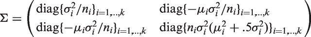
Let $t = ({\bar{x}}_{1}, …, {\bar{x}}_{k}, - .5 S_{1}^{* 2}, …, - .5 S_{2}^{* 2})',$ , where $S_{i}^{* 2} = \sum_{j = 1}^{n_{i}} X_{i j}^{2}, i = 1, …, k$ . Let $\hat{θ}$ be the estimate of $θ$ obtained by replacing the components of $θ$ by their usual MLEs, and $\tilde{θ}$ be the estimate obtained by replacing the components by the constrained MLEs under H₀. Define $\hat{Σ}, \tilde{Σ}$ , and $\tilde{τ}$ similarly. Let

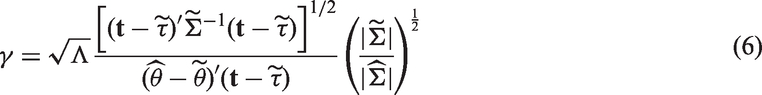
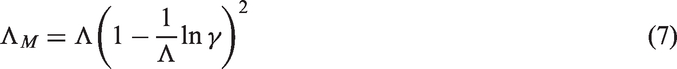
\begin{matrix} γ = \sqrt{Λ} \frac{[(t - \tilde{τ})' {\tilde{Σ}}^{- 1} (t - \tilde{τ})]^{1 / 2}}{(\hat{θ} - \tilde{θ})' (t - \tilde{τ})} (\frac{| \tilde{Σ} |}{| \hat{Σ} |})^{\frac{1}{2}} \end{matrix}

(6)

In terms of these quantities, the MLRT statistic is expressed as

Λ_{M} = Λ (1 - \frac{1}{Λ} \ln γ)^{2}

(7)

This test rejects H₀ in equation (1) when $Λ_{M} > χ_{k - 1; 1 - α}^{2} .$

Remark 1

It should be noted that the quantity γ in equation (6) could be negative for some samples, because the term $Q = (\hat{θ} - \tilde{θ})' (t - \tilde{τ})$ in the denominator could be negative. For such cases, the test statistic Λ _M is not defined. For example, when $(n_{1}, \dots, n_{4}) = (24, 10, 4, 37), (μ_{1}, \dots, μ_{4}) = (4.6, 4.6, 4.8, 4.6)$ and $(σ_{1}, \dots, σ_{4}) = (. 10, . 10, . 11, . 25)$ , a Monte Carlo simulation consisting of 100,000 runs indicated that Q could be negative 96.6% of times; for the same sample sizes with different parameters $(μ_{1}, \dots, μ_{4}) = (3.76, 3.47, 4.05, 3.80)$ and $(σ_{1}, \dots, σ_{4}) = (. 11, . 15, . 06, . 14)$ , Q is negative 89.7% of times. In fact, for the example data in Table 8, it can be readily checked that $(\hat{θ} - \tilde{θ})' (t - \tilde{τ}) = - 868.94$ and for the data in Table 9, it is −239.32. Thus, the MLRT is not applicable for both sets of data.

2.2 The standardized likelihood ratio test

We now consider an alternative approach to improve the LRT. Let $m (Λ)$ and $SD (Λ)$ denote the mean and standard deviation of Λ, respectively. We can standardize the Λ as

Λ_{S} = \sqrt{2 (k - 1)} (\frac{Λ - m (Λ)}{SD (Λ)}) + (k - 1)

(8)

which has an approximate

χ_{k - 1}^{2}

distribution. We refer to the test based on Λ _S as the standardized LRT (SLRT), and this SLRT rejects H₀ when

Λ_{S} > χ_{k - 1; 1 - α}^{2}

or the p value

P (χ_{k - 1}^{2} > Λ_{S}) < α

. In a general setup, DiCiccio et al.²⁶ have argued that such standardization improves the LRT, and the SLRT is third-order accurate in the sense that the approximation to the

χ_{k - 1}^{2}

distribution is

O (n^{- \frac{3}{2}})

. Notice that in the present setup, Λ _S is determined so that the mean and the variance of Λ _S are the same as those of the

χ_{k - 1}^{2}

distribution, and so the

χ_{k - 1}^{2}

approximation to the null distribution of Λ _S is expected to be accurate. Even though we do not know the order of accuracy, our simulation results in Section 2.5 clearly indicate that the SLRT based on Λ _S is practically exact even for small samples. Expressions for

m (Λ)

and

SD (Λ)

are difficult to obtain, and so we shall estimate them using simulated samples from

N ({\hat{η}}_{c} - . 5 σ_{1 c}^{2}, {\hat{σ}}_{1 c}^{2}), \dots, N ({\hat{η}}_{c} - . 5 σ_{kc}^{2}, {\hat{σ}}_{kc}^{2})

as suggested by DiCiccio et al.²⁶ for a general case. We refer to the test based on equation (8) as the SLRT, and it can be carried out using the following algorithm.

Algorithm 1

For a given set of k log-transformed samples, calculate $({\bar{X}}_{i}, V_{i}^{2}), i = 1, \dots, k$ .

Calculate the constrained MLEs ${\hat{η}}_{c}$ and $({\hat{σ}}_{1 c}^{2}, \dots, {\hat{σ}}_{kc}^{2})$ , and the LRT statistic Λ in equation (5).

Generate a sample of size n_i from the $N ({\hat{η}}_{c} - . 5 {\hat{σ}}_{ic}^{2}, {\hat{σ}}_{ic}^{2}), i = 1, \dots, k$ .

Calculate the SLRT statistic for the samples generated in the previous step.

Repeat the steps 2 and 3 for a large number of times, say, 10,000.

Find the mean and SD of these 10,000 simulated SLRT statistics, and standardize the Λ as in equation (8).

If the SLRT statistic is greater than $χ_{k - 1; 1 - α}^{2}$ , rejects the H₀ in equation (1).

2.3 The GV approach

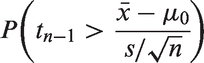
The GV approach is a special case of the fiducial method introduced by Fisher.²⁷ To outline this approach in the present context, consider testing $H_{0} : μ = μ_{0}$ vs. $H_{a} : μ > μ_{0}$ based on $\bar{X}$ and S, where $\bar{X}$ and S are, respectively, the mean and standard deviation of a random sample of size n from a $N (μ, σ^{2})$ distribution. For an observed value $(\bar{x}, s)$ of $(\bar{X}, S)$ , the p value is given by

\begin{matrix} P (t_{n - 1} > \frac{\bar{x} - μ_{0}}{s / \sqrt{n}}) \end{matrix}

For a given level of significance α, the “probable values” of μ are the set of μ determined by

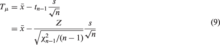
\begin{matrix} {μ : P (t_{n - 1} > \frac{\bar{x} - μ}{s / \sqrt{n}}) > α}, or equivalently {μ : P (\bar{x} - t_{n - 1} \frac{s}{\sqrt{n}} < μ) > α} \end{matrix}

Thus, for a given $(\bar{x}, s)$ , the fiducial variable for the parameter μ is given by

\begin{matrix} T_{μ} = \bar{x} - t_{n - 1} \frac{s}{\sqrt{n}} \\ = \bar{x} - \frac{Z}{\sqrt{χ_{n - 1}^{2} / (n - 1)}} \frac{s}{\sqrt{n}} \end{matrix}

(9)

where

Z \sim N (0, 1)

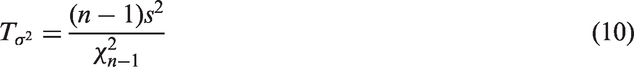
independently of

χ_{n - 1}^{2}

. Similarly, it can be shown that the fiducial distribution for

σ^{2}

T_{σ^{2}} = \frac{(n - 1) s^{2}}{χ_{n - 1}^{2}}

(10)

Weerahandi^28,29 has provided a recipe to find such fiducial quantities in a general setup, and referred to them as “generalized variable” or “generalized pivotal quantity (GPQ).” A GPQ for a function of parameters can be obtained by substitution. For example, the GPQ for $η = μ + \frac{1}{2} σ^{2}$ is given by $T_{η} = T_{μ} + \frac{1}{2} σ^{2}$ . For more details in the present context, see Krishnamoorthy and Mathew.¹⁷

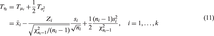
To describe the GV test for the equality of several log-normal means, let $({\bar{X}}_{i}, S_{i}^{2})$ denote the (mean, variance) based on a random sample of n_i observations from a $N (μ_{i}, σ_{i}^{2})$ distribution, $i = 1, \dots, k$ . Here $S_{i}^{2}$ is the usual unbiased estimate of $σ_{i}^{2}$ with denominator $n_{i} - 1$ . Let $({\bar{x}}_{i}, s_{i})$ be an observed value of $({\bar{X}}_{i}, S_{i}), i = 1, \dots, k$ . The GPQ for η_i follows from equations (9) and (10), and is given by

\begin{matrix} T_{η_{i}} = T_{μ_{i}} + \frac{1}{2} T_{σ_{i}^{2}} \\ = {\bar{x}}_{i} - \frac{Z_{i}}{\sqrt{χ_{n_{i} - 1}^{2} / (n_{i} - 1)}} \frac{s_{i}}{\sqrt{n_{i}}} + \frac{1}{2} \frac{(n_{i} - 1) s_{i}^{2}}{χ_{n_{i} - 1}^{2}}, i = 1, \dots, k \end{matrix}

(11)

where

Z_{i} \sim N (0, 1)

, and Z_is and

χ_{n_{i} - 1}^{2}

are mutually independent.

For the special case of k = 2, the GPQ for testing equation (15) is obtained by substitution, and is given by

T_{η_{1} - η_{2}} = T_{η_{1}} - T_{η_{2}}

(12)

where

T_{η_{i}}

is defined in equation (11). The generalized p value for testing equation (15) is given by

P (T_{η_{1}} - T_{η_{2}} < 0)

. It is clear from equation (11) that, for a given

({\bar{x}}_{1}, s_{1}, {\bar{x}}_{2}, s_{2})

, the distribution of

T_{η_{1} - η_{2}}

does not depend on any unknown parameters, and so the generalized p value can be estimated by Monte Carlo simulation.

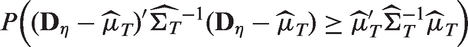
For $k \geq 3$ , there is no unique way of finding the GPQ, and we shall describe the approach by Li.²² Let

D_{η} = (T_{η_{1}} - T_{η_{k}}, \dots, T_{η_{k - 1}} - T_{η_{k}})

(13)

Let

{\hat{μ}}_{T}

be an estimate of

μ_{T} = E (D_{η} | \bar{x}, s)

, where

\bar{x} = ({\bar{x}}_{1}, \dots, {\bar{x}}_{k})

and

s = (s_{1}, \dots, s_{k})

. Let

{\hat{Σ}}_{T}

be an estimate of

Σ_{T} = Cov (D_{η} | \bar{x}, s)

. For a given

(\bar{x}, s)

, the generalized p value is given by

\begin{matrix} P ((D_{η} - {\hat{μ}}_{T})' {\hat{Σ_{T}}}^{- 1} (D_{η} - {\hat{μ}}_{T}) \geq \hat{μ}'_{T} {\hat{Σ}}_{T}^{- 1} {\hat{μ}}_{T}) \end{matrix}

The GV test rejects the null hypothesis in equation (1) if the generalized p value is less than the nominal level α. Li²² has provided the following Algorithm 2 to estimate the generalized p value.

Algorithm 2

For a given $(n_{1}, \dots, n_{k}), \bar{x}$ and s:

Generate $U_{i}^{2} \sim χ_{n_{i} - 1}^{2}$ and $Z_{i} \sim N (0, 1), i = 1, \dots, k$ .

Calculate $D_{η}$ .

Repeat steps 1–2 for a large number of times, say, M.

Calculate the mean and covariance of these M values of $D_{η}$ , and denote it by ${\hat{μ}}_{T}$ , and calculate the covariance matrix based on these M values of $D_{η}$ , and denote it by ${\hat{Σ}}_{T} .$

Compute $\hat{μ}'_{T} {\hat{Σ}}_{T}^{- 1} {\hat{μ}}_{T}$ .

Compute $Q^{*} = (D_{η} - {\hat{μ}}_{T})' {\hat{Σ}}_{T}^{- 1} (D_{η} - {\hat{μ}}_{T})$ , for each of M generated values of $D_{η}$ .

The percentage of the $Q^{*}$ s that are greater than $\hat{μ}'_{T} {\hat{Σ}}_{T}^{- 1} {\hat{μ}}_{T}$ is an estimate of the generalized p value.

It should be noted that $Σ_{T}$ exists only when all sample sizes are 6 or more (see equation (2.6) of Li²²), and so for smaller samples it is possible to have nearly singular ${\hat{Σ}}_{T}$ . As a result, implementation of the above algorithm could pose some problems for small sample sizes, because in such cases the estimate ${\hat{Σ}}_{T}$ could be nearly singular, and not invertible. Indeed, we encountered such computational problems in our simulation study in the sequel.

2.4 Two-sample case: one-sided tests

2.4.1 The SLRT

For one-sided tests of comparing two means, we can use the following statistic given by

Z = sign (({\bar{X}}_{1} + . 5 V_{1}^{2}) - ({\bar{X}}_{2} + . 5 V_{2}^{2})) \sqrt{Λ}

(14)

where the LRT statistic Λ is given in equation (5) with k = 2. For testing

H_{0} : η_{1} \leq η_{2} vs H_{a} : η_{1} > η_{2}

(15)

the SLRT rejects H₀ at the level α when

(Z - \hat{m} (Z)) / \hat{SD} (Z) > z_{1 - α}

, where

(\hat{m} (Z), \hat{SD} (Z))

denotes the estimated (mean, standard deviation) of Z, and z_q denotes the 100q percentile of the standard normal distribution.

2.4.2 Test based on MOVER CI

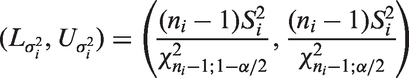
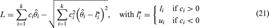
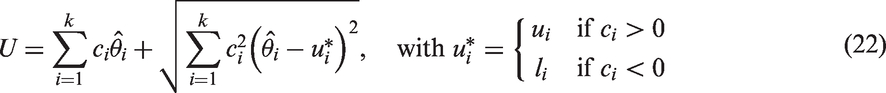
Zou and Donner³⁰ and Zou et al.^24,31 have proposed the MOVER, which is useful to find an approximate CI for a linear combination of parameters based on CIs of the individual parameters. Consider a linear combination $\sum_{i = 1}^{k} c_{i} θ_{i}$ of parameters $θ_{1}, \dots, θ_{g}$ , where c_is are known constants. Let ${\hat{θ}}_{1}, \dots, {\hat{θ}}_{g}$ be independent unbiased estimates of $θ_{1}, \dots, θ_{g}$ . Further, let (l_i, u_i) denote the $1 - α$ CI for θ_i, $i = 1, \dots, g$ . The $1 - α$ MOVER CI (L, U) for $\sum_{i = 1}^{g} c_{i} θ_{i}$ can be expressed as

L = \sum_{i = 1}^{g} c_{i} {\hat{θ}}_{i} - \sqrt{\sum_{i = 1}^{g} c_{i}^{2} ({\hat{θ}}_{i} - l_{i}^{*})^{2}}, with l_{i}^{*} = {\begin{matrix} l_{i} & if c_{i} > 0 \\ u_{i} & if c_{i} < 0 \end{matrix}

(16)

and

\begin{matrix} U = \sum_{i = 1}^{g} c_{i} {\hat{θ}}_{i} + \sqrt{\sum_{i = 1}^{g} c_{i}^{2} ({\hat{θ}}_{i} - u_{i}^{*})^{2}}, with u_{i}^{*} = {\begin{matrix} u_{i} & if c_{i} > 0 \\ l_{i} & if c_{i} < 0 \end{matrix} \end{matrix}

(17)

Graybill and Wang³² first obtained the above CI for a linear combination of variance components, and refer to their approach as the modified large sample method. Zou and coauthors gave a Wald type argument so as to the above CI is valid for any parameters; see Zou and Donner,³⁰ Zou et al.^24,31 These authors refer to the CIs of the above form as the MOVER CIs.

For the present problem, Zou et al.²⁴ have proposed the following approximate CI for the ratio of log-normal means based on the MOVER. To express the CI for $η_{i} = μ_{i} + σ_{i}^{2} / 2$ , let

(L_{μ_{i}}, U_{μ_{i}}) = {\bar{X}}_{i} \mp z_{1 - α / 2} \frac{S_{i}}{{\sqrt{n}}_{i}}, i = 1, 2

(18)

where z_q denotes the 100q percentile of the standard normal distribution, and let

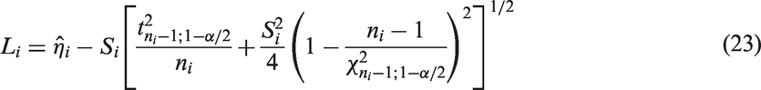
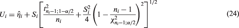
\begin{matrix} (L_{σ_{i}^{2}}, U_{σ_{i}^{2}}) = (\frac{(n_{i} - 1) S_{i}^{2}}{χ_{n_{i} - 1; 1 - α / 2}^{2}}, \frac{(n_{i} - 1) S_{i}^{2}}{χ_{n_{i} - 1; α / 2}^{2}}) \end{matrix}

The $1 - α$ MOVER CI for η_i is given by $(L_{η_{i}}, U_{η_{i}})$ , where

L_{η_{i}} = {\bar{X}}_{i} + \frac{1}{2} S_{i}^{2} - \sqrt{({\bar{X}}_{i} - L_{μ_{i}})^{2} + \frac{1}{4} (S_{i}^{2} - L_{σ_{i}^{2}})^{2}}

(19)

and

U_{η_{i}} = {\bar{X}}_{i} + \frac{1}{2} S_{i}^{2} + \sqrt{({\bar{X}}_{i} - U_{μ_{i}})^{2} + \frac{1}{4} (S_{i}^{2} - U_{σ_{i}^{2}})^{2}}

(20)

We can use the CIs of the form (19) and (20) for η₁ and η₂, to find a MOVER CI for $η_{1} - η_{2}$ . Let $(L_{η_{i}}, U_{η_{i}})$ be the $1 - α$ MOVER CI for η_i based on $({\bar{Y}}_{i}, S_{i})$ , i = 1, 2. Let

{\hat{η}}_{i} = {\bar{X}}_{i} + \frac{1}{2} S_{i}^{2}, i = 1, 2

Then, the MOVER CI for $η_{1} - η_{2}$ is given by (L_D, U_D), where

L_{D} = {\hat{η}}_{1} - {\hat{η}}_{2} - \sqrt{({\hat{η}}_{1} - L_{η_{1}})^{2} + ({\hat{η}}_{2} - U_{η_{2}})^{2}}

and

U_{D} = {\hat{η}}_{1} - {\hat{η}}_{2} + \sqrt{({\hat{η}}_{1} - U_{η_{1}})^{2} + ({\hat{η}}_{2} - L_{η_{2}})^{2}}

In terms of (L_D, U_D), the MOVER CI for the ratio of means is given by $(exp (L_{D}), exp (U_{D})) .$ For more details on the MOVER, see Zou and Donner³⁰ and Zou et al.³¹

A test based on the above CI rejects the null hypothesis $H_{0} : η_{1} = η_{2}$ whenever the CI for the ratio of means does not include one.

2.5 Type I error rates and power studies

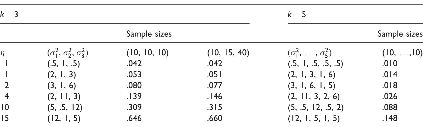
As noted earlier, the MLRT is not even defined for some samples. However, for some sample size and parameter configurations, we found that the quantity

(\hat{θ} - \tilde{θ})' (t - \tilde{τ})

in equation (6) is positive for all simulated samples, and so we could evaluate the type I error rates. Using Monte Carlo simulation consisting of 100,000 runs, we estimated type I error rates of the MLRT for the cases of k = 3 and k = 5, and some sample sizes no less than 10, and reported them in Table 1. These type I error rates clearly indicate that the MLRT proposed in Gill²¹ could be conservative for small values of η (the unknown common parameter under H₀ in equation (1)) or too liberal for large values of η. In some cases, the type I error rate could be as large as .66 when the nominal level is .05 (see Table 1). For these reasons, we shall not include this MLRT for further comparison studies.

Table 1.

Type I error rates of the MLRT.

k = 3				k = 5
		Sample sizes		Sample sizes
η	$(σ_{1}^{2}, σ_{2}^{2}, σ_{3}^{2})$	(10, 10, 10)	(10, 15, 40)	$(σ_{1}^{2}, \dots, σ_{5}^{2})$	(10, …,10)
1	(.5, 1, .5)	.042	.042	(.5, 1, .5, .5, .5)	.010
1	(2, 1, 3)	.053	.051	(2, 1, 3, 1, 6)	.014
2	(3, 1, 6)	.080	.077	(3, 1, 6, 1, 5)	.018
4	(2, 11, 3)	.139	.146	(2, 11, 3, 2, 6)	.026
10	(5, .5, 12)	.309	.315	(5, .5, 12, .5, 2)	.088
15	(12, 1, 5)	.646	.660	(12, 1, 5, 1, 5)	.148

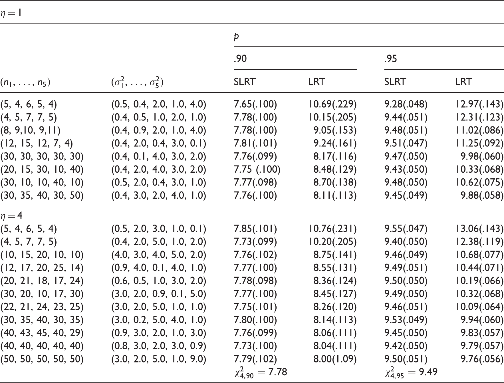
To judge the improvement of the SLRT over the LRT based on the asymptotic chi-square distribution, we estimated the percentiles of the SLRT statistic Λ _S and those of the LRT statistic Λ using Monte Carlo simulation consisting of 100,000 runs. Simulation estimates of the percentiles were obtained for the case of k = 5 with the parameter values of η = 1 and 4, and for various values of

(σ_{1}^{2}, \dots, σ_{5}^{2})

. These estimated percentiles along with the percentiles of the chi-square distribution with 4 degrees of freedom are presented in Table 2. We see in Table 2 that the percentiles of the SLRT statistic Λ _S practically coincide with those of the

χ_{4}^{2}

distribution. Thus, the chi-square approximation to the SLRT statistic is quite accurate even for small samples. The

χ^{2}

approximation to the LRT statistic Λ is not accurate even for moderately large samples. In general, the estimated percentiles of the LRT statistic are greater than the corresponding

χ_{4}^{2}

percentiles, which implies that the LRT based on the chi-square approximation could be liberal when it is applied for small to moderate samples; see the type I error rates in parentheses. The estimated error rates of the LRT indicate that the LRT is liberal even when all sample sizes are 40, while the SLRT is very satisfactory for all sample sizes. We also evaluated the powers of the LRT and SLRT (not reported here) for some sample size and parameter configurations. The powers of the tests are quite similar for samples of sizes 50 or more. For small to moderate samples, the LRT is slightly more powerful than the SLRT. This is because for small to moderate sample sizes, the LRT has inflated type I error rates, as a result, it appears to be more powerful than the SLRT.

Table 2.

The 100p percentiles and (type I error rates) of the SLRT and LRT statistics.

η = 1
$(n_{1}, \dots, n_{5})$	$(σ_{1}^{2}, \dots, σ_{5}^{2})$	p
		.90		.95
		SLRT	LRT	SLRT	LRT
(5, 4, 6, 5, 4)	(0.5, 0.4, 2.0, 1.0, 4.0)	7.65(.100)	10.69(.229)	9.28(.048)	12.97(.143)
(4, 5, 7, 7, 5)	(0.4, 0.5, 1.0, 2.0, 1.0)	7.78(.100)	10.15(.205)	9.44(.051)	12.31(.123)
(8, 9,10, 9,11)	(0.4, 0.9, 2.0, 1.0, 4.0)	7.78(.100)	9.05(.153)	9.48(.051)	11.02(.086)
(12, 15, 12, 7, 4)	(0.4, 2.0, 0.4, 3.0, 0.1)	7.81(.101)	9.24(.161)	9.51(.047)	11.25(.092)
(30, 30, 30, 30, 30)	(0.4, 0.1, 4.0, 3.0, 2.0)	7.76(.099)	8.17(.116)	9.47(.050)	9.98(.060)
(20, 15, 30, 10, 40)	(0.4, 2.0, 4.0, 3.0, 2.0)	7.75 (.100)	8.48(.129)	9.43(.050)	10.33(.068)
(30, 10, 10, 40, 10)	(0.5, 2.0, 0.4, 3.0, 1.0)	7.77(.098)	8.70(.138)	9.48(.050)	10.62(.075)
(30, 35, 40, 30, 50)	(0.4, 3.0, 2.0, 4.0, 1.0)	7.76(.100)	8.11(.113)	9.45(.049)	9.88(.058)
η = 4
(5, 4, 6, 5, 4)	(0.5, 2.0, 3.0, 1.0, 0.1)	7.85(.101)	10.76(.231)	9.55(.047)	13.06(.143)
(4, 5, 7, 7, 5)	(0.4, 2.0, 5.0, 1.0, 2.0)	7.73(.099)	10.20(.205)	9.40(.050)	12.38(.119)
(10, 15, 20, 10, 10)	(4.0, 3.0, 4.0, 5.0, 2.0)	7.76(.102)	8.75(.141)	9.46(.049)	10.68(.077)
(12, 17, 20, 25, 14)	(0.9, 4.0, 0.1, 4.0, 1.0)	7.77(.100)	8.55(.131)	9.49(.051)	10.44(.071)
(20, 21, 18, 17, 24)	(0.6, 0.5, 1.0, 3.0, 2.0)	7.78(.098)	8.36(.124)	9.50(.050)	10.19(.066)
(30, 20, 10, 17, 30)	(3.0, 2.0, 0.9, 0.1, 5.0)	7.77(.100)	8.45(.127)	9.49(.050)	10.32(.068)
(22, 21, 24, 23, 25)	(3.0, 2.0, 5.0, 1.0, 1.0)	7.75(.101)	8.26(.120)	9.46(.051)	10.09(.064)
(30, 35, 40, 30, 35)	(3.0, 0.2, 5.0, 4.0, 1.0)	7.80(.100)	8.14(.113)	9.53(.049)	9.94(.060)
(40, 43, 45, 40, 29)	(0.9, 3.0, 2.0, 1.0, 3.0)	7.76(.099)	8.06(.111)	9.45(.050)	9.83(.057)
(40, 40, 40, 40, 40)	(0.8, 3.0, 2.0, 3.0, 0.9)	7.73(.100)	8.04(.111)	9.42(.050)	9.79(.057)
(50, 50, 50, 50, 50)	(3.0, 2.0, 5.0, 1.0, 9.0)	7.79(.102)	8.00(1.09)	9.50(.051)	9.76(.056)
		$χ_{4, . 90}^{2} = 7.78$		$χ_{4, . 95}^{2} = 9.49$

To judge the performance of the SLRT, MOVER test and the GV test, we performed various simulation studies and estimated the type I error rates and powers of both tests for small to moderate samples. The type I error rates of the SLRT are estimated as follows. We first generated 10,000 samples each of size n_i from a $N (η - . 5 σ_{i}^{2}, σ_{i}^{2}), i = 1, \dots, k .$ For each set of k generated samples, the SLRT was carried out using Algorithm 1 with M = 1000. The percentage of rejections is a Monte Carlo estimate of the type I error rates. The type I error rates of the GV test is estimated similarly, and the type I error rates of the MOVER test are estimated using simulation consisting of 10,000 runs.

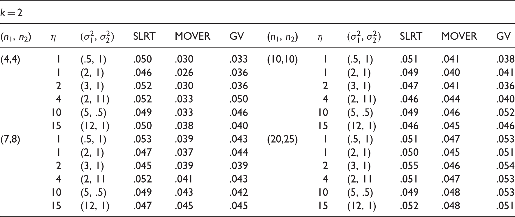
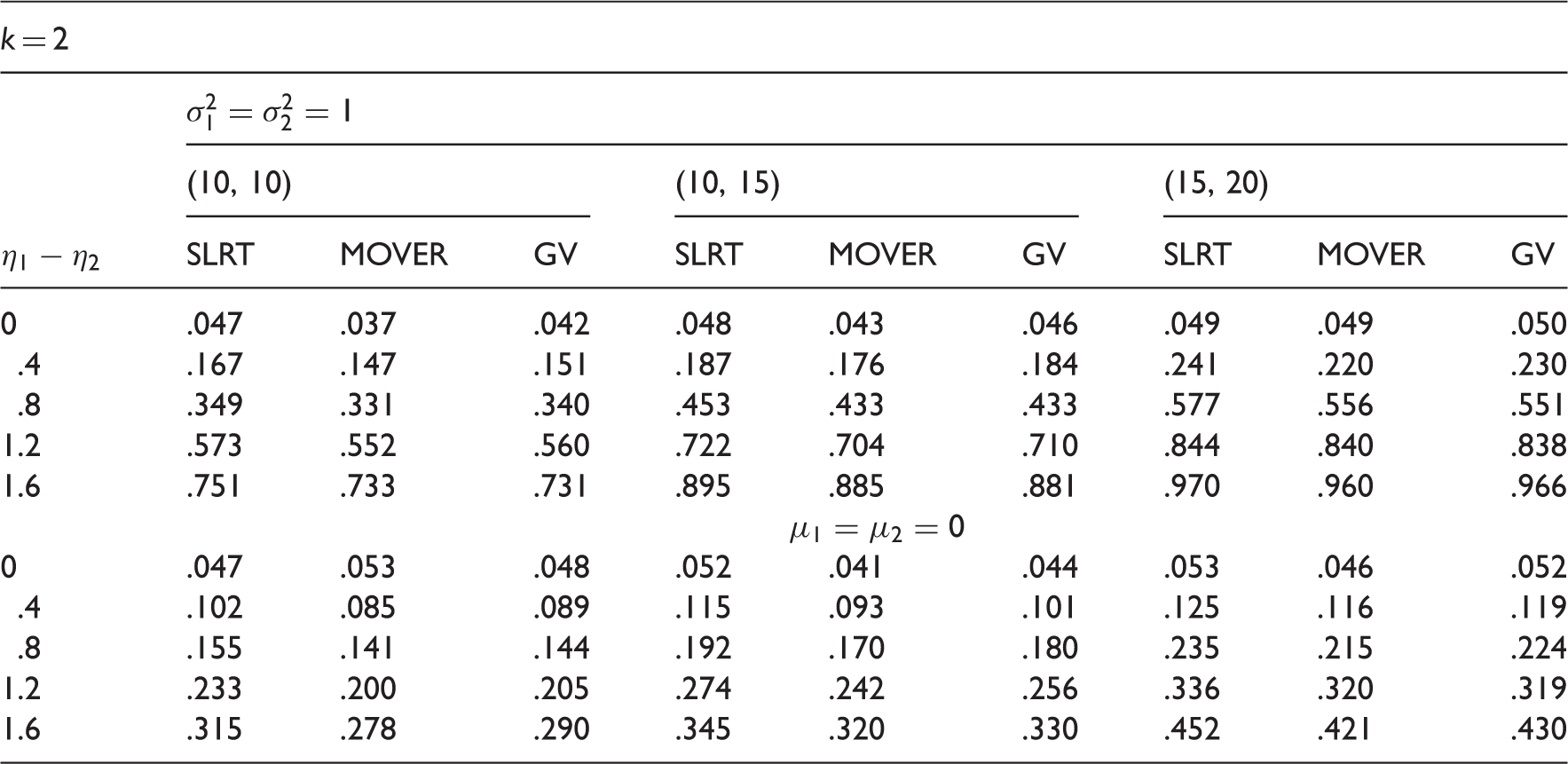
The type I error rates of the SLRT, MOVER and the GV test are presented in Table 3 for the case of k = 2. The type I error rates clearly indicate that the SLRT controls the error rates very close to the nominal level .05. The MOVER test and the GV test appears to be conservative for small samples, and they also perform satisfactorily for moderate samples. The estimated powers of the tests for one-sided hypotheses are given in Table 4. The powers in the first part of Table 4 are for various values of

η_{1} - η_{2} \geq 0

while

σ_{i}^{2}

s are fixed at one. Comparison of the powers of these three tests indicates that the SLRT is more powerful than the other two tests. The powers in the second part of Table 4 are for various values of

η_{1} - η_{2}

while μ₁ and μ₂ are fixed at zero. We once again notice that the powers of the SLRT are greater than those of the other two tests. Overall, the SLRT may be preferred to the MOVER test and the GV test for small to moderate sample sizes.

Table 3.

Type I error rates of the tests for $H_{0} : η_{1} = η_{2}$ vs. $H_{a} : η_{1} \neq η_{2}$ .

k = 2
(n₁, n₂)	η	$(σ_{1}^{2}, σ_{2}^{2})$	SLRT	MOVER	GV	(n₁, n₂)	η	$(σ_{1}^{2}, σ_{2}^{2})$	SLRT	MOVER	GV
(4,4)	1	(.5, 1)	.050	.030	.033	(10,10)	1	(.5, 1)	.051	.041	.038
	1	(2, 1)	.046	.026	.036		1	(2, 1)	.049	.040	.041
	2	(3, 1)	.052	.030	.036		2	(3, 1)	.047	.041	.036
	4	(2, 11)	.052	.033	.050		4	(2, 11)	.046	.044	.040
	10	(5, .5)	.049	.033	.046		10	(5, .5)	.049	.046	.052
	15	(12, 1)	.050	.038	.040		15	(12, 1)	.046	.045	.046
(7,8)	1	(.5, 1)	.053	.039	.043	(20,25)	1	(.5, 1)	.051	.047	.053
	1	(2, 1)	.047	.037	.044		1	(2, 1)	.050	.045	.051
	2	(3, 1)	.045	.039	.039		2	(3, 1)	.055	.046	.054
	4	(2, 11	.052	.041	.043		4	(2, 11	.051	.047	.053
	10	(5, .5)	.049	.043	.042		10	(5, .5)	.049	.048	.053
	15	(12, 1)	.047	.045	.045		15	(12, 1)	.052	.048	.051

Table 4.

Powers of the tests for $H_{0} : η_{1} \leq η_{2}$ vs. $H_{a} : η_{1} > η_{2}$ .

k = 2
	$σ_{1}^{2} = σ_{2}^{2} = 1$
	(10, 10)			(10, 15)			(15, 20)
$η_{1} - η_{2}$	SLRT	MOVER	GV	SLRT	MOVER	GV	SLRT	MOVER	GV
0	.047	.037	.042	.048	.043	.046	.049	.049	.050
.4	.167	.147	.151	.187	.176	.184	.241	.220	.230
.8	.349	.331	.340	.453	.433	.433	.577	.556	.551
1.2	.573	.552	.560	.722	.704	.710	.844	.840	.838
1.6	.751	.733	.731	.895	.885	.881	.970	.960	.966
	$μ_{1} = μ_{2} = 0$
0	.047	.053	.048	.052	.041	.044	.053	.046	.052
.4	.102	.085	.089	.115	.093	.101	.125	.116	.119
.8	.155	.141	.144	.192	.170	.180	.235	.215	.224
1.2	.233	.200	.205	.274	.242	.256	.336	.320	.319
1.6	.315	.278	.290	.345	.320	.330	.452	.421	.430

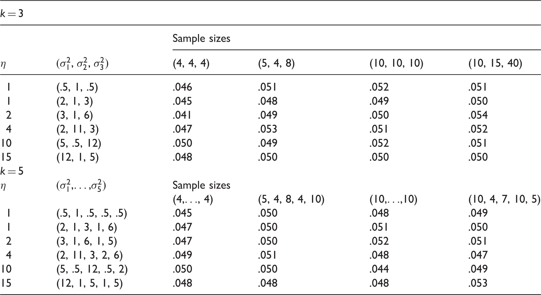
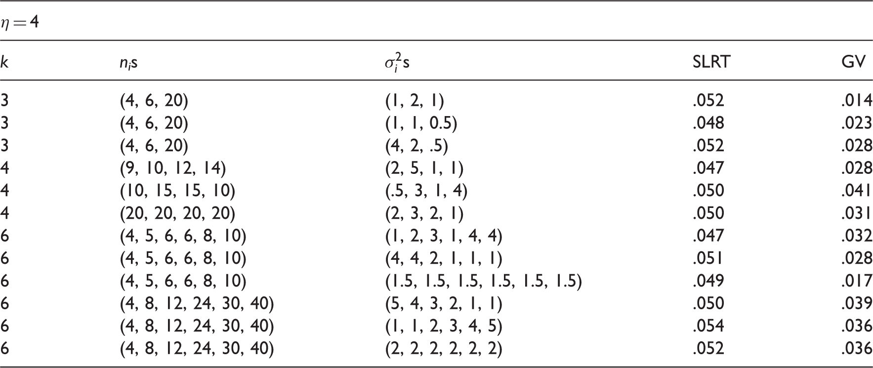
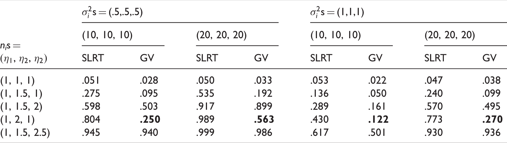
To see the small sample behavior of the SLRT for the cases of k > 2, we estimated the type I error rates of the SLRT for k = 3 and k = 5 and reported in Table 5. The estimated error rates clearly indicate that the SLRT is very satisfactory even for samples of size 4. We evaluated the GV test for sample size configurations as given in Table 2 of Li.²² For these sample sizes and k = 3, 4 and 6, type I error rates of the GV test and the SLRT are given in Table 6. We once again observe from these table values that the SLRT is very satisfactory in controlling type I error rates whereas the GV test is conservative, as a consequence, the GV test is expected to be less powerful than the SLRT. To see the gain in power by using the SLRT, we estimated the powers of the tests for some moderate sample sizes and presented them in Table 7. Comparison of estimated powers clearly shows that the SLRT is much more powerful than the GV test. Furthermore, the GV test has a peculiar power property; the power is decreasing with increasing disparity among η_is. For example, we see in Table 7 that the power of the test at the sample sizes (10, 10, 10) and

(η_{1}, η_{2}, η_{3}) = (1, 1.5, 2)

is .503, and at (1, 2, 1) is .250, while for the same cases the power of the SLRT increased from .598 to .804. Also, see the powers of the GV test when sample sizes are (10, 10, 10) and

(σ_{1}^{2}, σ_{2}^{2}, σ_{3}^{2}) = (1, 1.5, 2)

and (1, 2, 1). This is an undesirable property for a test, because the power of a test should increase with increasing disparity among the values of ηs.

Table 5.

Type I error rates of the SLRT.

k = 3
η	$(σ_{1}^{2}, σ_{2}^{2}, σ_{3}^{2})$	Sample sizes
η	$(σ_{1}^{2}, σ_{2}^{2}, σ_{3}^{2})$	(4, 4, 4)	(5, 4, 8)	(10, 10, 10)	(10, 15, 40)
1	(.5, 1, .5)	.046	.051	.052	.051
1	(2, 1, 3)	.045	.048	.049	.050
2	(3, 1, 6)	.041	.049	.050	.054
4	(2, 11, 3)	.047	.053	.051	.052
10	(5, .5, 12)	.050	.049	.052	.051
15	(12, 1, 5)	.048	.050	.050	.050
k = 5
η	$(σ_{1}^{2}, \dots, σ_{5}^{2})$	Sample sizes
η	$(σ_{1}^{2}, \dots, σ_{5}^{2})$	(4,…, 4)	(5, 4, 8, 4, 10)	(10,…,10)	(10, 4, 7, 10, 5)
1	(.5, 1, .5, .5, .5)	.045	.050	.048	.049
1	(2, 1, 3, 1, 6)	.047	.050	.051	.050
2	(3, 1, 6, 1, 5)	.047	.050	.052	.051
4	(2, 11, 3, 2, 6)	.049	.051	.048	.047
10	(5, .5, 12, .5, 2)	.050	.050	.044	.049
15	(12, 1, 5, 1, 5)	.048	.048	.048	.053

Table 6.

Type I errors of the SLRT and the GV test.

η = 4
k	n_is	$σ_{i}^{2}$ s	SLRT	GV
3	(4, 6, 20)	(1, 2, 1)	.052	.014
3	(4, 6, 20)	(1, 1, 0.5)	.048	.023
3	(4, 6, 20)	(4, 2, .5)	.052	.028
4	(9, 10, 12, 14)	(2, 5, 1, 1)	.047	.028
4	(10, 15, 15, 10)	(.5, 3, 1, 4)	.050	.041
4	(20, 20, 20, 20)	(2, 3, 2, 1)	.050	.031
6	(4, 5, 6, 6, 8, 10)	(1, 2, 3, 1, 4, 4)	.047	.032
6	(4, 5, 6, 6, 8, 10)	(4, 4, 2, 1, 1, 1)	.051	.028
6	(4, 5, 6, 6, 8, 10)	(1.5, 1.5, 1.5, 1.5, 1.5, 1.5)	.049	.017
6	(4, 8, 12, 24, 30, 40)	(5, 4, 3, 2, 1, 1)	.050	.039
6	(4, 8, 12, 24, 30, 40)	(1, 1, 2, 3, 4, 5)	.054	.036
6	(4, 8, 12, 24, 30, 40)	(2, 2, 2, 2, 2, 2)	.052	.036

Table 7.

Powers of the SLRT and the GV test.

	$σ_{i}^{2}$ s = (.5,.5,.5)				$σ_{i}^{2}$ s = (1,1,1)
n_is =	(10, 10, 10)		(20, 20, 20)		(10, 10, 10)		(20, 20, 20)
$(η_{1}, η_{2}, η_{2})$	SLRT	GV	SLRT	GV	SLRT	GV	SLRT	GV
(1, 1, 1)	.051	.028	.050	.033	.053	.022	.047	.038
(1, 1.5, 1)	.275	.095	.535	.192	.136	.050	.240	.099
(1, 1.5, 2)	.598	.503	.917	.899	.289	.161	.570	.495
(1, 2, 1)	.804	.250	.989	.563	.430	.122	.773	.270
(1, 1.5, 2.5)	.945	.940	.999	.986	.617	.501	.930	.936

2.6 An example for comparing log-normal means

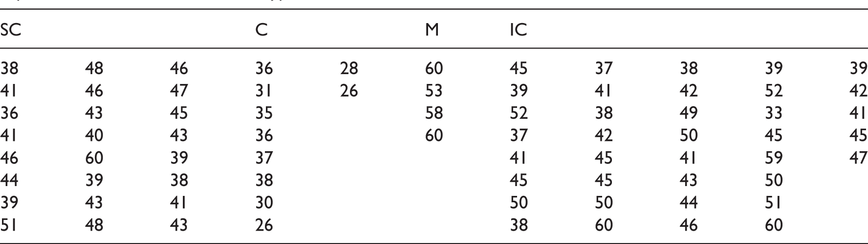
Let us now illustrate the methods in the preceding sections, using the example described in Section 1.1. Recall that there are four TAPVR subtypes, namely, SC = group 1, C = group 2, M = group 3 and IC = group 4. The data on deep hypothermic circulatory arrest time on these four groups are given in Table 8. As noted in Section 1.1, the data in group 3 do not satisfy the log-normality assumption, and so we compare only groups 1, 2 and 4. The sample sizes

(n_{1}, n_{2}, n_{4}) = (24, 10, 37)

, the sample means and SDs of log-transformed data are

({\bar{x}}_{1}, {\bar{x}}_{2}, {\bar{x}}_{4}) =

(3.7675, 3.4654, 3.7944) and

(s_{1}, s_{2}, s_{4}) = (. 1123, . 1474, . 1411)

. To apply the SLRT for equality of means, the constrained MLEs were calculated as

{\hat{η}}_{c} = 3.785 and ({\hat{σ}}_{1 c}^{2}, {\hat{σ}}_{2 c}^{2}, {\hat{σ}}_{4 c}^{2}) = (. 01237, . 11844, . 01271)

Table 8.

Deep hypothermic circulatory arrest time (in minutes) of four anatomical TAPVR subtypes; SC, supracardiac; C, cardiac; M, mixed type; IC, infracardiac.

SC			C		M	IC
38	48	46	36	28	60	45	37	38	39	39
41	46	47	31	26	53	39	41	42	52	42
36	43	45	35		58	52	38	49	33	41
41	40	43	36		60	37	42	50	45	45
46	60	39	37			41	45	41	59	47
44	39	38	38			45	45	43	50
39	43	41	30			50	50	44	51
51	48	43	26			38	60	46	60

The LRT statistic was computed as $Λ = 16.36$ with the estimated mean $\hat{m} (Λ) = 2.211$ and the estimated $\hat{SD} (Λ) = 2.210$ . The mean and SD were estimated using Algorithm 1 with M = 100, 000. Noting that k = 3, the SLRT statistic equation (8) is

\sqrt{4} \times \frac{16.36 - 2.21}{2.21} + 2 = 14.80

The p value is $P (χ_{2}^{2} > 14.80) = . 0006 .$ The GV statistic $\hat{μ}'_{T} {\hat{Σ}}_{T}^{- 1} {\hat{μ}}_{T} = 32.02$ and the generalized p value is .0002. Thus, both SLRT and the GV test reject the null hypothesis of equal group means at any practical level of significance.

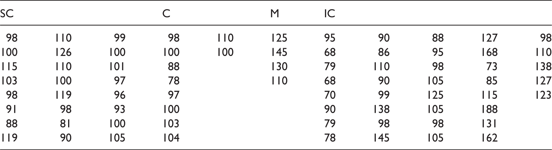
Prolonged cardiopulmonary bypass time (data are in Table 9) is also a known adverse outcome, or a risk factor of mortality in the repair of TAPVR (Friesen et al.³³). The data for the cardiac group do not satisfy log-normal assumption; nevertheless, we shall include this group for comparison. The statistics for the cardiopulmonary bypass time (in minutes) of the four anatomical TAPVR subtypes are as follows: As in the previous example, let SC = group 1, C = group 2, M = group 3 and IC = group 4. Then

(n_{1}, n_{2}, n_{3}, n_{4}) = (24, 10, 4, 37), ({\bar{x}}_{1}, {\bar{x}}_{2}, {\bar{x}}_{3}, {\bar{x}}_{4}) = (4.6154, 4.5789, 4.8433, 4.6373)

and

(s_{1}, s_{2}, s_{3}, s_{4}) = (. 1027, . 0966, . 1140, . 2547)

. The constrained MLEs

({\hat{η}}_{c}, {\hat{σ}}_{1 c}^{2}, \dots, {\hat{σ}}_{4 c}^{2}) = (4.623, . 0101, . 0103, . 0574, . 0623)

Table 9.

Prolonged cardiopulmonary bypass time (in minutes) of four anatomical TAPVR subtypes; SC, supracardiac; C, cardiac; M, mixed type; IC, infracardiac.

SC			C		M	IC
98	110	99	98	110	125	95	90	88	127	98
100	126	100	100	100	145	68	86	95	168	110
115	110	101	88		130	79	110	98	73	138
103	100	97	78		110	68	90	105	85	127
98	119	96	97			70	99	125	115	123
91	98	93	100			90	138	105	188
88	81	100	103			79	98	98	131
119	90	105	104			78	145	105	162

The LRT statistic is 11.006 with the estimated mean of 3.72 and the estimated SD of 3.06. The SLRT statistic Λ _S in equation (8) is 8.84 and the p value is $P (χ_{3}^{2} > 8.84) = . 031 .$ The GV test yielded $\hat{μ}'_{T} {\hat{Σ}}_{T}^{- 1} {\hat{μ}}_{T} = 4.75$ and the generalized p value is .121. For this example, we see that the SLRT rejects the null hypothesis of equal means at 5% level, whereas the GV test does not reject. This is in agreement with our simulation studies which indicated that the GV test is less powerful than the SLRT.

3 CIs for the common mean

Consider k log-normal populations with parameters $(μ_{1}, σ_{1}), \dots, (μ_{k}, σ_{k})$ . Assume that the means of these k populations are the same $exp (η)$ , where $η = (μ_{i} + . 5 σ_{i}^{2}), i = 1, \dots, k$ . Tian and Wu¹⁹ proposed a GV approach for finding a CI for the common mean of several log-normal distributions. We shall develop a simple closed-form approximate CI for the common mean based on the MOVER, and also propose a modification to the GV test due to Tian and Wu.¹⁹

3.1 MOVER CI for the common mean

The MOVER CI for a linear combination of parameters $θ_{1}, \dots, θ_{k}$ is described as follows. Let ${\hat{θ}}_{i}$ be an unbiased estimate of θ_i, $i = 1, \dots, k$ . Assume that ${\hat{θ}}_{1}, \dots, {\hat{θ}}_{k}$ are independent. Further, let (l_i, u_i) denote the $1 - α$ CI for θ_i, $i = 1, \dots, k$ . The $1 - α$ MOVER CI (L, U) for $\sum_{i = 1}^{k} c_{i} θ_{i}$ can be expressed as

\begin{matrix} L = \sum_{i = 1}^{k} c_{i} {\hat{θ}}_{i} - \sqrt{\sum_{i = 1}^{k} c_{i}^{2} ({\hat{θ}}_{i} - l_{i}^{*})^{2}}, with l_{i}^{*} = {\begin{matrix} l_{i} & if c_{i} > 0 \\ u_{i} & if c_{i} < 0 \end{matrix} \end{matrix}

(21)

and

\begin{matrix} U = \sum_{i = 1}^{k} c_{i} {\hat{θ}}_{i} + \sqrt{\sum_{i = 1}^{k} c_{i}^{2} ({\hat{θ}}_{i} - u_{i}^{*})^{2}}, with u_{i}^{*} = {\begin{matrix} u_{i} & if c_{i} > 0 \\ l_{i} & if c_{i} < 0 \end{matrix} \end{matrix}

(22)

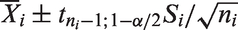
Notice that the above method can be used to obtain a CI for the common η by combining the individual CIs for $μ_{i} + . 5 σ_{i}^{2}$ based on ${\bar{X}}_{i}$ and $S_{i}^{2}$ . A closed-form CI for $μ_{i} + . 5 σ_{i}^{2}$ can also be obtained by combining the z-interval

{\bar{X}}_{i} \pm t_{n_{i} - 1; 1 - α / 2} S_{i} / \sqrt{n_{i}}

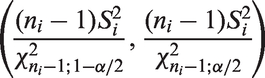
for μ_i and the usual CI

\begin{matrix} (\frac{(n_{i} - 1) S_{i}^{2}}{χ_{n_{i} - 1; 1 - α / 2}^{2}}, \frac{(n_{i} - 1) S_{i}^{2}}{χ_{n_{i} - 1; α / 2}^{2}}) \end{matrix}

for

σ_{i}^{2}, i = 1, \dots, k

(see Zou et al.³¹). Specifically, the MOVER CI for

μ_{i} + . 5 σ_{i}^{2}

is given by

(L_{i}, U_{i})

, where

\begin{matrix} L_{i} = {\hat{η}}_{i} - S_{i} [\frac{t_{n_{i} - 1; 1 - α / 2}^{2}}{n_{i}} + \frac{S_{i}^{2}}{4} (1 - \frac{n_{i} - 1}{χ_{n_{i} - 1; 1 - α / 2}^{2}})^{2}]^{1 / 2} \end{matrix}

(23)

and

\begin{matrix} U_{i} = {\hat{η}}_{i} + S_{i} [\frac{t_{n_{i} - 1; 1 - α / 2}^{2}}{n_{i}} + \frac{S_{i}^{2}}{4} (1 - \frac{n_{i} - 1}{χ_{n_{i} - 1; α / 2}^{2}})^{2}]^{1 / 2} \end{matrix}

(24)

where

{\hat{η}}_{i} = {\bar{X}}_{i} + . 5 S_{i}^{2}, i = 1, \dots, k

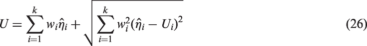
A CI, say, (L, U) for the common parameter η can be obtained by combining these independent CIs of η as

L = \sum_{i = 1}^{k} w_{i} {\hat{η}}_{i} - \sqrt{\sum_{i = 1}^{k} w_{i}^{2} ({\hat{η}}_{i} - L_{i})^{2}}

(25)

and

U = \sum_{i = 1}^{k} w_{i} {\hat{η}}_{i} + \sqrt{\sum_{i = 1}^{k} w_{i}^{2} ({\hat{η}}_{i} - U_{i})^{2}}

(26)

where

w_{i} = (n_{i} / S_{i}^{2}) / \sum_{j = 1}^{k} (n_{j} / S_{j}^{2}) .

Notice that w_is are chosen so that the weight for the CI based on the ith sample is inversely proportional to the sample variance, and directly proportional to the ith sample size. One could also choose w_i as inversely proportional to an estimate of the variance of

{\hat{η}}_{i} = {\bar{X}}_{i} + \frac{S_{i}^{2}}{2}

. Our choice of w_is is not only simple, but also our preliminary simulation studies (not reported here) indicated that the CI formed by equations (25) and (26) is better than the CI based on other values of w_is in terms of coverage probabilities. For these reasons, we chose to use the w_is defined above.

Remark 2

Zou et al.²⁴ used the z-interval ${\bar{X}}_{i} \pm z_{1 - α / 2} S_{i} / \sqrt{n_{i}}$ for μ_i for estimating a log-normal mean using the MOVER. MOVER CIs based on such z-intervals work satisfactorily for finding a CI for a log-normal mean or for the difference between two log-normal means as shown in Section 2.4. However, for the present problem, our preliminary studies indicated that the CI for the common parameter $μ + . 5 σ^{2}$ based on z-intervals is slightly liberal, and the coverage probability could be appreciably lower than the nominal level. So we propose t intervals for μ_i instead of the z-intervals. Henceforth we refer to the CI for the common parameter η on the basis of z-intervals for μ_i as the MOVER-z CI, and the one on the basis of t intervals for μ_i as the MOVER-t CI.

3.2 GV approach

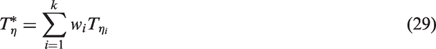
We shall now describe the GV approach for finding CIs for the common mean of several log-normal distributions. Let $R_{η}^{(i)} = exp (T_{η_{i}})$ , where $T_{η_{i}}$ is the GPQ for $η = μ_{i} + . 5 σ_{i}^{2}$ given in equation (11). Let

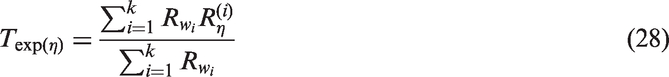
T_{μ_{i}} = {\bar{x}}_{i} - \frac{Z_{i}}{U_{i} / \sqrt{n_{i} - 1}} \frac{s_{i}}{\sqrt{n_{i}}} and T_{σ_{i}^{2}} = \frac{s_{i}^{2}}{U_{i}^{2} / (n_{i} - 1)}, i = 1, \dots,, k

(27)

Furthermore, let $R_{w_{i}} = [T_{σ_{i}^{2}} (1 + T_{σ_{i}^{2}} / 2) exp (2 T_{μ_{i}} + T_{σ_{i}^{2}})]^{- 1} .$ In terms of these quantities, the GPQ for the common mean is expressed as

T_{exp (η)} = \frac{\sum_{i = 1}^{k} R_{w_{i}} R_{η}^{(i)}}{\sum_{i = 1}^{k} R_{w_{i}}}

(28)

The above GPQ was developed by Tian and Wu.¹⁹ Our preliminary simulation studies on the coverage probabilities of the CIs based on $T_{exp (η)}$ indicated that the CIs could be very liberal for some parameter and sample size configurations. As an alternative, we propose the following GPQ for η from which a CI for the common mean $exp (η)$ can be readily obtained. The alternative GPQ for η is given by

T_{η}^{*} = \sum_{i = 1}^{k} w_{i} T_{η_{i}}

(29)

where

T_{η_{i}}

s are given in equation (11), and

w_{i} = (n_{i} / s_{i}^{2}) / (\sum_{j = 1}^{k} n_{j} / s_{j}^{2}), j = 1, \dots, k

. Note that for a given

({\bar{x}}_{1}, \dots, {\bar{x}}_{k}, s_{1}^{2}, \dots, s_{k}^{2})

, the distribution of

T_{η}^{*}

does not depend on any unknown parameters, and so its percentiles can be estimated using Monte Carlo simulation. The lower and upper

100 α

percentiles form a 100

(1 - 2 α)

% CI for the common parameter η.

3.3 Coverage studies for the common mean

The properties of the CIs for the common mean of several log-normal distributions can be judged from those of the CIs for the common η. To judge the coverage properties and precisions of the CIs for the common parameter η, we estimated their coverage probabilities and expected widths using Monte Carlo simulation. The coverage probabilities of the MOVER CIs are estimated by simulation consisting of 100,000 runs. The coverage probabilities of the generalized CIs are estimated as follows. We first generated 2500 independent samples of size n_i from a $N (η - . 5 σ_{i}^{2}, σ_{i}^{2})$ distribution, $i = 1, \dots, k$ , with some assumed parameters. For each set of generated samples, we computed the generalized CI using simulation consisting of 5000 runs. The percentage of CIs that include the assumed common mean is a Monte Carlo estimate of the coverage probability.

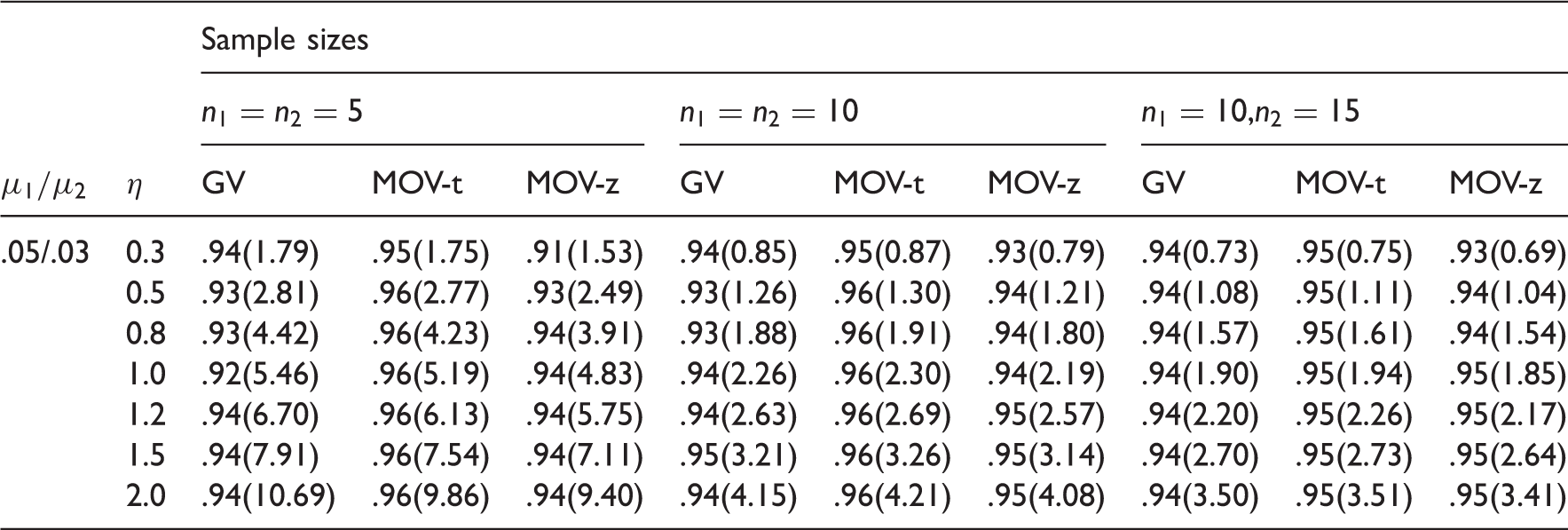
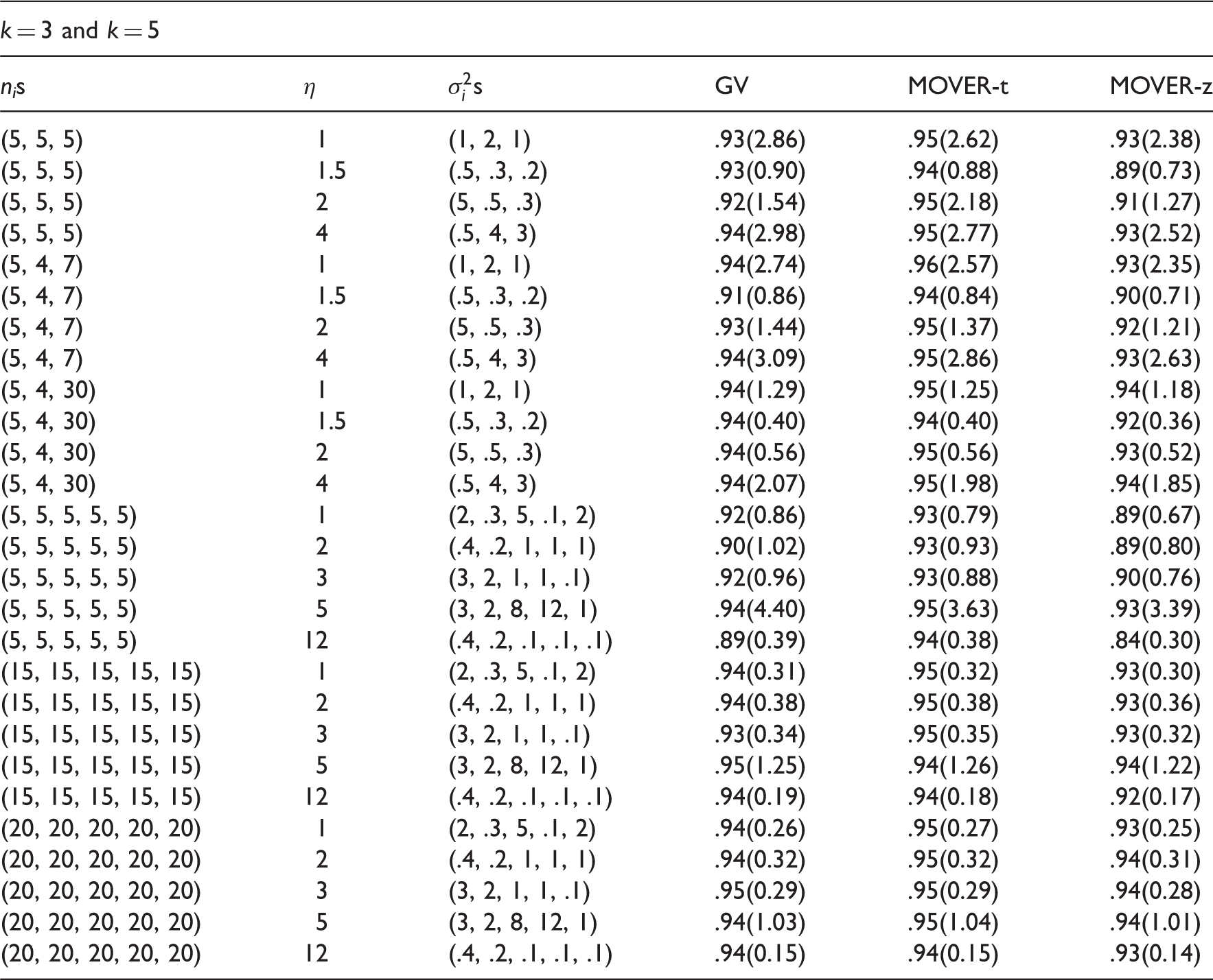
For the two-sample case, we estimated the coverage probabilities and expected widths of the CIs by the GV method, MOVER-t (MOV-t) and MOVER-z (MOV-z) for some parameter configurations considered in Table 1 of Tian and Wu.¹⁹ The estimated coverage probabilities along with the expected widths are given in Table 10. Examination of coverage probabilities clearly indicate that the MOVER-t CIs are very satisfactory in controlling coverage probabilities very close to the nominal level .95. The GV CIs and MOVER-z CIs are also satisfactory except that they could be liberal in some situations. We also note that expected widths of the MOVER CIs are quite comparable with those of generalized CIs when their coverage probabilities are the same. Comparison for the case of

(n_{1}, n_{2}) = (5, 5)

, the MOVER-t CIs have better coverage probabilities with smaller expected widths than the generalized CIs. The MOVER-z CIs are also simple to compute, but their coverage probabilities could go as low as .91 when the nominal level is .95. Estimated coverage probabilities and expected widths of CIs are reported in Table 11 for cases of k = 3 and 5. We once again observe from the table values that the MOVER-t CIs outperform the generalized CIs in terms coverage probabilities and precision. The MOVER-z CIs could be liberal, and in some cases their coverage probabilities could go as low as .84 when the nominal level is .95; see the result for the case of

(n_{1}, \dots, n_{5}) = (5, \dots, 5)

and η = 12. Notice that we reported coverage probabilities for small to moderate samples, because for large samples all three CIs perform similarly. Overall we see that the MOVER-t CIs are accurate, simple to compute and better than the other two CIs in terms of coverage probabilities.

Table 10.

Coverage probabilities and (expected widths) of 95% CIs for the common mean; k = 2.

$μ_{1} / μ_{2}$	η	Sample sizes
		$n_{1} = n_{2} = 5$			$n_{1} = n_{2} = 10$			$n_{1} = 10, n_{2} = 15$
		GV	MOV-t	MOV-z	GV	MOV-t	MOV-z	GV	MOV-t	MOV-z
.05/.03	0.3	.94(1.79)	.95(1.75)	.91(1.53)	.94(0.85)	.95(0.87)	.93(0.79)	.94(0.73)	.95(0.75)	.93(0.69)
	0.5	.93(2.81)	.96(2.77)	.93(2.49)	.93(1.26)	.96(1.30)	.94(1.21)	.94(1.08)	.95(1.11)	.94(1.04)
	0.8	.93(4.42)	.96(4.23)	.94(3.91)	.93(1.88)	.96(1.91)	.94(1.80)	.94(1.57)	.95(1.61)	.94(1.54)
	1.0	.92(5.46)	.96(5.19)	.94(4.83)	.94(2.26)	.96(2.30)	.94(2.19)	.94(1.90)	.95(1.94)	.95(1.85)
	1.2	.94(6.70)	.96(6.13)	.94(5.75)	.94(2.63)	.96(2.69)	.95(2.57)	.94(2.20)	.95(2.26)	.95(2.17)
	1.5	.94(7.91)	.96(7.54)	.94(7.11)	.95(3.21)	.96(3.26)	.95(3.14)	.94(2.70)	.95(2.73)	.95(2.64)
	2.0	.94(10.69)	.96(9.86)	.94(9.40)	.94(4.15)	.96(4.21)	.95(4.08)	.94(3.50)	.95(3.51)	.95(3.41)

Table 11.

Coverage probabilities of 95% CIs for the common mean.

k = 3 and k = 5
n_is	η	$σ_{i}^{2}$ s	GV	MOVER-t	MOVER-z
(5, 5, 5)	1	(1, 2, 1)	.93(2.86)	.95(2.62)	.93(2.38)
(5, 5, 5)	1.5	(.5, .3, .2)	.93(0.90)	.94(0.88)	.89(0.73)
(5, 5, 5)	2	(5, .5, .3)	.92(1.54)	.95(2.18)	.91(1.27)
(5, 5, 5)	4	(.5, 4, 3)	.94(2.98)	.95(2.77)	.93(2.52)
(5, 4, 7)	1	(1, 2, 1)	.94(2.74)	.96(2.57)	.93(2.35)
(5, 4, 7)	1.5	(.5, .3, .2)	.91(0.86)	.94(0.84)	.90(0.71)
(5, 4, 7)	2	(5, .5, .3)	.93(1.44)	.95(1.37)	.92(1.21)
(5, 4, 7)	4	(.5, 4, 3)	.94(3.09)	.95(2.86)	.93(2.63)
(5, 4, 30)	1	(1, 2, 1)	.94(1.29)	.95(1.25)	.94(1.18)
(5, 4, 30)	1.5	(.5, .3, .2)	.94(0.40)	.94(0.40)	.92(0.36)
(5, 4, 30)	2	(5, .5, .3)	.94(0.56)	.95(0.56)	.93(0.52)
(5, 4, 30)	4	(.5, 4, 3)	.94(2.07)	.95(1.98)	.94(1.85)
(5, 5, 5, 5, 5)	1	(2, .3, 5, .1, 2)	.92(0.86)	.93(0.79)	.89(0.67)
(5, 5, 5, 5, 5)	2	(.4, .2, 1, 1, 1)	.90(1.02)	.93(0.93)	.89(0.80)
(5, 5, 5, 5, 5)	3	(3, 2, 1, 1, .1)	.92(0.96)	.93(0.88)	.90(0.76)
(5, 5, 5, 5, 5)	5	(3, 2, 8, 12, 1)	.94(4.40)	.95(3.63)	.93(3.39)
(5, 5, 5, 5, 5)	12	(.4, .2, .1, .1, .1)	.89(0.39)	.94(0.38)	.84(0.30)
(15, 15, 15, 15, 15)	1	(2, .3, 5, .1, 2)	.94(0.31)	.95(0.32)	.93(0.30)
(15, 15, 15, 15, 15)	2	(.4, .2, 1, 1, 1)	.94(0.38)	.95(0.38)	.93(0.36)
(15, 15, 15, 15, 15)	3	(3, 2, 1, 1, .1)	.93(0.34)	.95(0.35)	.93(0.32)
(15, 15, 15, 15, 15)	5	(3, 2, 8, 12, 1)	.95(1.25)	.94(1.26)	.94(1.22)
(15, 15, 15, 15, 15)	12	(.4, .2, .1, .1, .1)	.94(0.19)	.94(0.18)	.92(0.17)
(20, 20, 20, 20, 20)	1	(2, .3, 5, .1, 2)	.94(0.26)	.95(0.27)	.93(0.25)
(20, 20, 20, 20, 20)	2	(.4, .2, 1, 1, 1)	.94(0.32)	.95(0.32)	.94(0.31)
(20, 20, 20, 20, 20)	3	(3, 2, 1, 1, .1)	.95(0.29)	.95(0.29)	.94(0.28)
(20, 20, 20, 20, 20)	5	(3, 2, 8, 12, 1)	.94(1.03)	.95(1.04)	.94(1.01)
(20, 20, 20, 20, 20)	12	(.4, .2, .1, .1, .1)	.94(0.15)	.94(0.15)	.93(0.14)

3.4 An example for estimating the common mean

As noted in Section 1.2, we shall illustrate the methods using the example given in Tian and Wu.¹⁹ The data set contains pharmacokinetics data from alcohol interaction study in men (Bradstreet and Liss²⁰). For illustrative purpose, we use the measurements* on maximum concentration (C_max) and compare the active treatment groups considered in Tian and Wu.¹⁹ The group sizes are equal with $n_{1} = n_{2} = n_{3} = 22$ . The sample mean ${\bar{x}}_{i}$ (sample variance $s_{i}^{2}$ ) of the log-transformed data are 2.601 (0.24), 2.596 (0.20) and 2.599 (0.17) for the three groups. It is desired to test

H_{0} : μ_{1} + . 5 σ_{1}^{2} = μ_{2} + . 5 σ_{2}^{2} = μ_{3} + . 5 σ_{3}^{2} vs . H_{a} : H_{0} is not true,

at the level .05.

The LRT statistic is computed as $Λ = . 0652$ with the estimated mean $\hat{m} (Λ) = 2.117$ and the estimated $\hat{SD} (Λ) = 2.104$ . The mean and SD were estimated based on 100,000 simulated samples each of size 22 from $N ({\hat{η}}_{c} - . 5 {\hat{σ}}_{1 c}^{2}, {\hat{σ}}_{1 c}^{2}), N ({\hat{η}}_{c} - . 5 {\hat{σ}}_{1 c}^{2}, {\hat{σ}}_{2 c}^{2})$ and $N ({\hat{η}}_{c} - . 5 {\hat{σ}}_{3 c}^{2})$ distributions. The SLRT statistic equation (8) is

\sqrt{4} \times \frac{. 0652 - 2.117}{2.104} + 2 = . 0497

The p value is $P (χ_{2}^{2} > . 0497) = . 975 .$ Thus, the equality of the group means is tenable.

Since the group means are not significantly different, it maybe desired to the find the common mean of these three groups. The MOVER-t CIs for the population means of C_max are (12.16, 19.52), (12.10,18.54), and (12.16, 17.94) for groups 1, 2 and 3, respectively. Using the proposed approach, the MOVER-t CI for the common mean is (13.22, 16.90), and the generalized CI is (13.37, 17.05). We estimated the generalized CI by Tian and Wu¹⁹ by simulation consisting of 100,000 runs as (13.17, 16.63). As noted earlier, the generalized CI by Tian and Wu¹⁹ is in general liberal, and so it produced the shortest CI among these three methods.

4 Conclusion

We have proposed a SLRT, and evaluated all available tests for the equality of several log-normal means. Our investigation showed that the MLRT is not appropriate for applications, because it is not even defined for some samples, and also it may have inflated type I error rates for some cases. Our simulation comparison indicates that the SLRT seems to be the best in terms of power and in controlling type I error rates around the nominal level. Even though the proposed SLRT involves simulation to estimate the mean and standard deviation of the LRT statistic, it can be easily implemented in a programming language such as R, MATLAB, SAS or Fortran. Interested readers can contact the first author for R codes. It should be noted that there are alternative modifications to the LRT available in the literature. Wu et al.³⁵ used one such modified approach to find a CI for the mean of a log-normal distribution. This modified version does not involve simulation, but it seems to be very difficult to extend it for comparing two or more log-normal means.

We have also investigated the problem of estimating the common mean of several log-normal populations, and proposed a closed-form approximate CI for the common mean. This closed-form CI is not only better than the GV CI, but also is easy to compute, and does not involve simulation.

Footnotes

Acknowledgments

The authors are thankful to Dr Joseph Caspi at LSUHSC for letting us use his TAPVR data. They are also grateful to two reviewers for providing useful comments and suggestions.

Declaration of conflicting interests

The author(s) declared no potential conflicts of interest with respect to the research, authorship, and/or publication of this article.

Funding

The author(s) received no financial support for the research, authorship, and/or publication of this article.

*The data are from Bradstreet and Liss20 and available at: .

Appendix 1

References

Radloff

. The CES-D Scale: a self-report depression scale for research in the general population. Appl Psychol Meas 1977; 1: 385–401.

Spencer

. Skewed distributions-new outcome measures. Community Dent Oral Epidemiol 1997; 25: 52–59.

Kotani

Kimura

Ebara

et al.

Serum aspirin esterase is strongly associated with glucose and lipids in healthy subjects: different association patterns in subjects with type 2 diabetes mellitus. Diabetol Metab Syndr 2010; 2: 50–62.

Danos D, Oral E, Simonsen N, et al. Lung cancer risk prediction with stochastic covariates. In: JSM proceedings, biometrics section, American Statistical Association, Alexandria, VA, 2012, pp.34–41.

Lee

. The lognormal distribution of growth rates of soft tissue metastases of breast cancer. J Surg Oncol 1972; 4: 82–88.

Bengtsson

Stahlberg

Rorsman

et al.

Gene expression profiling in single cells from the pancreatic islets of Langerhans reveals lognormal distribution of mRNA levels. Genom Res 2005; 15: 1388–1392.

Neti

PVSV

Howell

. Log-normal distribution of cellular uptake of radioactivity: statistical analysis of alpha particle track autoradiography. J Nucl Med 2006; 47: 1049–1058.

Limpert

Stahel

Abbt

. Log-normal distributions across the sciences: keys and clues. BioScience 2001; 51: 341–352.

Heath

. Normal or log-normal: appropriate distributions. Nature 1967; 213: 1159–1160.

10.

Sorrentino

. Large standard deviations and logarithmic-normality. BioScience 2010; 4: 327–332.

11.

Rappaport

Selvin

. A method for evaluating the mean exposure from a log-normal distribution. Am Ind Hyg Assoc J 1987; 48: 374–379.

12.

Selvin

Rappaport

. Note on the estimation of the mean value from a log-normal distribution. Am Ind Hyg Assoc J 1989; 50: 627–630.

13.

Krishnamoorthy

Mathew

Ramachandran

. Generalized p-values and confidence limits: a novel approach for analyzing lognormally distributed exposure data. J Occup Environ Hyg 2006; 3: 252–260.

14.

Griswold

Parmigiani

Potosky

et al.

Analyzing health care costs: a comparison of statistical methods motivated by medicare colorectal cancer charges. Biostatistics 2004; 1: 1–23.

15.

Shen

Brown

Zhi

. Efficient estimation of log-normal means with application to pharmacokinetic data. Stat Med 2006; 25: 3023–3038.

16.

Zhou

Gao

Hui

. Methods for comparing the means of two independent log-normal samples. Biometrics 1997; 53: 1129–1135.

17.

Krishnamoorthy

Mathew

. Inferences on the means of log-normal distributions using generalized p-values and generalized confidence intervals. J Stat Plann Inference 2003; 115: 103–121.

18.

Hirsch

Bove

. Total anomalous pulmonary venous connection. Multimedia Man Cardiothorac Surg 2007; 22: 1–7. DOI:10.1510/mmcts.2006.002253.

19.

Tian

. Inferences on the common mean of several log-normal populations: the generalized variable approach. Biometrical J 2007; 49: 944–951.

20.

Bradstreet TE and Liss CL. Favorite data sets from early (and late) phases of drug research - Part 4. In: Proceedings of the Section on Statistical Education of the American Statistical Association, 1995.

21.

Gill

. Small-sample inference for the comparison of means of log-normal distributions. Biomterics 2004; 60: 525–527.

22.

. A generalized p-value approach for comparing the means of several log-normal populations. Stat Probabil Lett 2009; 79: 1404–1408.

23.

Welsh

. Aspects of statistical inference, Hoboken, NJ: Wiley, 1996.

24.

Zou

Taleban

Huo

. Simple confidence intervals for log-normal means and their differences with environmental applications. Environmetrics 2009; 20: 172–180.

25.

Skovgaard

. Likelihood asymptotics. Scand J Stat 2001; 28: 3–32.

26.

DiCiccio

Martin

Stern

. Simple and accurate one-sided inference from signed roots of likelihood ratios. Canadian J Stat 2001; 29: 67–76.

27.

Fisher

. The fiducial argument in statistical inference. Ann Eugenics 1935; 8: 391–398.

28.

Weerahandi

. Generalized confidence intervals. J Am Stat Assoc 1993; 88: 899–905.

29.

Weerahandi

. Exact statistical methods for data analysis, New York, NY: Springer-Verlag, 1995.

30.

Zou

Donner

. Construction of confidence limits about effect measures: a general approach. Stat Med 2008; 27: 1693–1702.

31.

Zou

Huo

Taleban

. Confidence interval estimation for log-normal data with application to health economics. Comp Stat Data Anal 2009; 53: 3755–3764.

32.

Graybill

Wang

. Confidence intervals on nonnegative linear combinations of variances. J Am Stat Assoc 1980; 75: 869–873.

33.

Friesen

CLH

Zurakowski

Thiagarajan

et al.

Total anomalous pulmonary venous connection: an analysis of current management strategies in a single institution. Ann Thorac Surg 2005; 79: 596–606.

34.

Krishnamoorthy

Lee

. Improved tests for the equality of normal coefficients of variation. Comput Stat 2013; 29: 215–232.

35.

Wong

ACM

Jiang

. Likelihood-based confidence intervals for a lognormal mean. Stat Med 2003; 22: 1849–1860.

SC			C		M	IC
38	48	46	36	28	60	45	37	38	39	39
41	46	47	31	26	53	39	41	42	52	42
36	43	45	35		58	52	38	49	33	41
41	40	43	36		60	37	42	50	45	45
46	60	39	37			41	45	41	59	47
44	39	38	38			45	45	43	50
39	43	41	30			50	50	44	51
51	48	43	26			38	60	46	60

SC			C		M	IC
98	110	99	98	110	125	95	90	88	127	98
100	126	100	100	100	145	68	86	95	168	110
115	110	101	88		130	79	110	98	73	138
103	100	97	78		110	68	90	105	85	127
98	119	96	97			70	99	125	115	123
91	98	93	100			90	138	105	188
88	81	100	103			79	98	98	131
119	90	105	104			78	145	105	162

SC			C		M	IC
38	48	46	36	28	60	45	37	38	39	39
41	46	47	31	26	53	39	41	42	52	42
36	43	45	35		58	52	38	49	33	41
41	40	43	36		60	37	42	50	45	45
46	60	39	37			41	45	41	59	47
44	39	38	38			45	45	43	50
39	43	41	30			50	50	44	51
51	48	43	26			38	60	46	60

SC			C		M	IC
98	110	99	98	110	125	95	90	88	127	98
100	126	100	100	100	145	68	86	95	168	110
115	110	101	88		130	79	110	98	73	138
103	100	97	78		110	68	90	105	85	127
98	119	96	97			70	99	125	115	123
91	98	93	100			90	138	105	188
88	81	100	103			79	98	98	131
119	90	105	104			78	145	105	162

SC			C		M	IC
38	48	46	36	28	60	45	37	38	39	39
41	46	47	31	26	53	39	41	42	52	42
36	43	45	35		58	52	38	49	33	41
41	40	43	36		60	37	42	50	45	45
46	60	39	37			41	45	41	59	47
44	39	38	38			45	45	43	50
39	43	41	30			50	50	44	51
51	48	43	26			38	60	46	60

SC			C		M	IC
98	110	99	98	110	125	95	90	88	127	98
100	126	100	100	100	145	68	86	95	168	110
115	110	101	88		130	79	110	98	73	138
103	100	97	78		110	68	90	105	85	127
98	119	96	97			70	99	125	115	123
91	98	93	100			90	138	105	188
88	81	100	103			79	98	98	131
119	90	105	104			78	145	105	162