Correcting for dependent censoring in routine outcome monitoring data by applying the inverse probability censoring weighted estimator

Abstract

Censored data make survival analysis more complicated because exact event times are not observed. Statistical methodology developed to account for censored observations assumes that patients’ withdrawal from a study is independent of the event of interest. However, in practice, some covariates might be associated to both lifetime and censoring mechanism, inducing dependent censoring. In this case, standard survival techniques, like Kaplan–Meier estimator, give biased results. The inverse probability censoring weighted estimator was developed to correct for bias due to dependent censoring. In this article, we explore the use of inverse probability censoring weighting methodology and describe why it is effective in removing the bias. Since implementing this method is highly time consuming and requires programming and mathematical skills, we propose a user friendly algorithm in R. Applications to a toy example and to a medical data set illustrate how the algorithm works. A simulation study was carried out to investigate the performance of the inverse probability censoring weighted estimators in situations where dependent censoring is present in the data. In the simulation process, different sample sizes, strengths of the censoring model, and percentages of censored individuals were chosen. Results show that in each scenario inverse probability censoring weighting reduces the bias induced in the traditional Kaplan–Meier approach where dependent censoring is ignored.

Keywords

Survival analysis informative censoring dependent censoring inverse probability censoring weighted estimator inverse probability weighting

1 Introduction

Survival analysis is the study of the distribution of lifetimes, i.e. the times from a pre specified initiating event (e.g. birth, diagnosis, start of treatment) to some terminal event of interest (e.g. death, relapse, remission). It is most prominently (but not exclusively) used in the biomedical sciences. A special feature of survival studies is that it takes time to observe the event of interest. As a result, for a number of subjects, the event is not observed during follow-up, and the only available information is that the event of interest has not taken place yet at the last observation time. This phenomenon is called censoring. Methodologies are developed to include censored subjects in analysis.

Standard methods used to analyze data with censored observations assume that censoring is non-informative. This means that censoring carries no prognostic information about the survival experience. Therefore, individuals who are censored at a specific time point should be as likely to experience an event as those subjects who remain in the study, i.e. the probability of being censored is the same for all subjects at risk. Informative censoring may occur when time to event and time to censoring are dependent, either directly or through covariates. In the latter case, dependence between event and censoring times is induced through covariates associated to time to event and time to censoring. This type of informative censoring is called dependent censoring and it is the focus of this article. For example, young patients may be more likely to quit a treatment than older patients. This implies that the event is observed more often in older than in young patients, leading to biased estimates of survival probabilities, because the observed event times are not representative for the event times of the whole population.

Since dependent censoring can cause bias in the results, it is crucial to consider this aspect in the analysis. Inverse probability censoring weighting (IPCW) was proposed^1–3 to correct for the presence of dependent censoring. This method is based on the idea of compensating for censored subjects by giving extra weight to subjects who are not censored. More specific, IPCW assigns extra weight to subjects with similar characteristics to the ones that are censored.

Implementing IPCW is very time consuming. Programming and mathematical skills are needed to apply the IPCW procedure, and careful bookkeeping is required. In this article, a user friendly implementation of IPCW in R is proposed. The algorithm makes clever use of the existing survival package. It makes the IPCW method more accessible to researchers.

As illustration, IPCW is applied to a toy data set and to a real data set from the Department of Psychiatry of the Leiden University Medical Center (LUMC) in The Netherlands. A simulation study is performed to compare IPCW with the traditional methodology in case dependent censoring is present in the data. Several scenarios were generated with different sample sizes, percentages of censoring, and strengths of the censoring mechanism. Simulations show that correcting for the presence of dependent censoring by using IPCW is crucial and reduces bias in the estimation results.

This article is organized as follows. Notation and a short introduction to techniques concerning survival analysis and details about the concept of dependent censoring are outlined in section 2. The IPCW method is illustrated and applied to a real data set in section 3. In section 4, a simulation study is presented in which the performance of IPCW is investigated. Details concerning the proposed user friendly implementation of the IPCW method in R are outlined in Supplementary Material A, and details concerning the simulation study are described in Supplementary Material B.

2 Dependent censoring in survival analysis

2.1 Definition dependent censoring

The aim of survival analysis is to estimate time to a certain event of interest, e.g. death or recovery. However, event times are often incompletely observed, i.e. time to the occurrence of the event of interest is not known for some subjects. This phenomenon is called censoring. Survival data for a subject j are represented as triplets $(t_{j}, δ_{j}, [Z_{j} (t), 0 \leq t \leq t_{j}])$ , where the observed variable t_j represents the survival time x_j if the event is observed ( $δ_{j} = 1$ ), or the censoring time c_j if the event is not observed ( $δ_{j} = 0$ ), i.e. $t_{j} = min (x_{j}, c_{j})$ . The vector of p (time-dependent) covariates is denoted by $Z_{j} (t) = (Z_{j 1} (t), \dots, Z_{jp} (t))^{t}$ . It is assumed that the value of $Z_{j} (t)$ is known at any time point in the subject’s observation time. Kaplan and Meier⁴ introduced the Product-Limit Estimator as an estimator for the marginal survival function (also referred to as Kaplan–Meier estimator). This estimator is defined as

\begin{matrix} \hat{S} (t) = {\begin{matrix} 1 & if t < t_{1} \\ \underset{t_{i} \leq t}{Π} [1 - \frac{d_{i}}{Y_{i}}] & if t \geq t_{1} \end{matrix}, \end{matrix}

(1)

where d_i and Y_i are, respectively, the number of events and the number of individuals at risk at time t_i. This estimator does not consider the covariates

Z_{j} (t)

in the survival curve estimation.

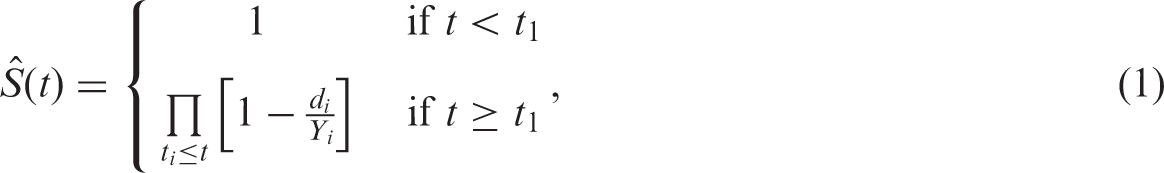
The Kaplan–Meier (KM) estimator assumes that censoring times are non-informative, i.e. that there is no dependence between lifetime X and censoring mechanism C. Hence, the hazard of X among subjects at risk is the marginal hazard of X, i.e.

h_{X} (t | C \geq t) = h_{X} (t),

(2)

or, equivalently, the hazard of censoring time C at time t does not depend on event time X

h_{C} (t | X, X > t) = h_{C} (t | X > t) .

(3)

This assumption may, however, be questionable in practice. For example, in situations where the covariates history

\bar{Z} (t) = {Z (x); 0 \leq x \leq t}

associated with event times also predicts censoring, i.e.

h_{C} (t | \bar{Z} (t), X > t) \neq h_{C} (t | X > t) .

(4)

A time-dependent Cox proportional hazard model for censoring can be used to test this condition. If equation (4) holds, event time X and censoring time C are dependent through covariates, a phenomenon called dependent censoring, and, as a consequence, equations (2) and (3) do not hold.³ In this case, estimators based on the independent censoring assumption, like KM estimator, should not be used.⁵ A proper methodology that accounts for dependent censoring should then be employed to avoid biased results.

To illustrate the possible bias when dependent censoring is present in the data under investigation, simulated data in which covariates are associated to both time to event and time to censoring are used to estimate the survival function. Results are given in Figure 1 where the traditional KM estimator and the real survival (which simply is the KM estimator in case all events times are observed) are shown together. For details concerning the simulations see Supplementary Material B.

Figure 1.

Real survival curve and Kaplan–Meier estimate in case dependent censoring is present in the data.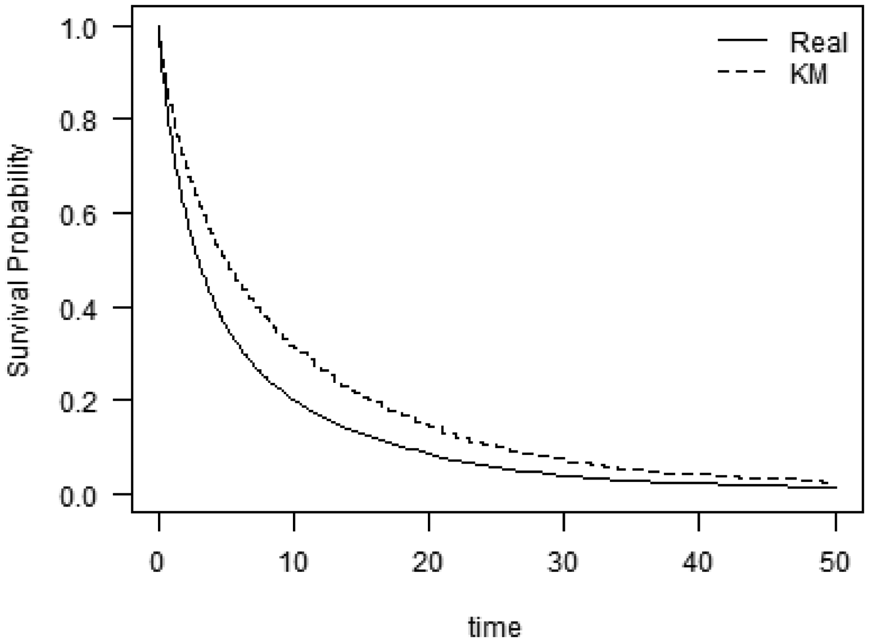

As expected the KM estimator overestimates the real survival probabilities. This indicates that correction for the presence of dependent censoring is important in order to obtain a good estimator. More examples are shown in the simulation study described in section 4.

2.2 IPCW estimator

The IPCW estimator^1–3 was developed to correct for dependent censoring. It corrects for censored subjects by giving extra weight to subjects who are not censored. Typically, these weights are chosen in such a way that individuals who best match the censored subjects will receive more weight. At every observed time point t, each subject j is given a weight which is inversely proportional to the estimated probability of having remained uncensored until time t. The estimated probability is based on the fit of a Cox model for censoring with risk factors for failure and censoring. When a subject is censored at time t_c, individuals who remain at risk should be given extra weight from t_c onward. Hence, IPCW weights have to be recalculated for each subject at risk at each censoring time. This procedure can be summarized in the four steps below.

Step 1

Fit a model for the censoring mechanism that incorporates covariates associated with event and censoring time.

Step 2

Estimate the probability of remaining uncensored at each observed time point t for all subjects at risk at that time point. Denote this estimated probability for subject j at time t as ${\hat{K}}_{j}^{Z} (t)$ .

Step 3

Compute the IPCW weights as ${\hat{W}}_{j} (t) = 1 / {\hat{K}}_{j}^{Z} (t)$ .

Step 4

Estimate the survival probabilities ${\hat{S}}_{IPCW} (t_{τ})$ for time to event in the absence of censoring with subjects weighted according to the IPCW methodology at each observed time point $t_{τ}$ of interest.

IPCW is based on the assumption that, given $\bar{Z} (t)$ , the hazard of C at time t is independent of the event time X, i.e.

h_{C} (t | \bar{Z} (t), X, X > t) = h_{C} (t | \bar{Z} (t), X > t) .

(5)

This means that all covariates that might be associated with event or censoring time must be measured, i.e. there should be no unmeasured confounders. If this assumption holds, in theory, IPCW can fully correct for bias due to dependent censoring. 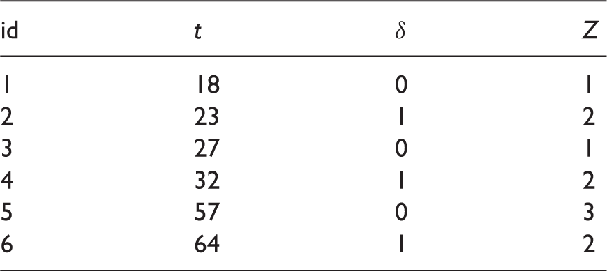Therefore, researchers should always gather enough prognostic values that are expected to influence censoring time, such that equation (5) may be approximately true.³ Even if all prognostic values are included in the model, a crucial step in the IPCW method is to have good estimates for the parameters in the censoring model. Small sample sizes, measurement errors, and other causes for a bad fit for the censoring model may reduce the precision of the estimated weights. However, when the fitted censoring model is accurate enough, the IPCW method will reduce the bias due to dependent censoring.

In the remainder of this section, details concerning the IPCW procedure are outlined. Data for subject j are denoted by

(t_{j}, δ_{j}, δ_{C_{j}}, [Z_{j} (t), 0 \leq t \leq t_{j}])

, where t_j is the observed time point, δ_j is the event indicator,

δ_{C_{j}} = 1 - δ_{j}

the censoring indicator and

Z_{j} (t)

the vector of covariate values at time t. To implement the IPCW procedure, careful bookkeeping, mathematical and programming skills are required, which makes implementation time consuming. In Supplementary Material A, a user friendly implementation of IPCW in R⁶ that uses the survival package^7,8 is proposed. Toy data in Table 1 are used to illustrate how the algorithm works.

Table 1.

Toy survival data for six subjects.

id	t	δ	Z
1	18	0	1
2	23	1	2
3	27	0	1
4	32	1	2
5	57	0	3
6	64	1	2

Note: For each subject, the observed time point t, event indicator δ and time-independent covariate Z are given.

2.2.1 Step 1: Fit censoring model

To assess the influence of covariates $Z (t)$ on the probability of being censored, these covariates are included in the Cox model for time to censoring

h_{C} (t | \bar{Z} (t)) = h_{C_{0}} (t) exp (β_{C}^{t} Z (t)),

(6)

where

h_{C_{0}}

is the baseline hazard,

β_{C}

is the vector of model parameters,

Z (t)

represents the covariates at time t, and

\bar{Z} (t)

the covariate history. Since this is a standard Cox model, existing methods to fit Cox models can be used for this step.

Fitting the Cox model for time to censoring on the toy data gives a hazard ratio of 0.281 for the covariate Z, with 95% confidence interval [0.031, 2.538]. This effect is not significant since no dependence between covariates and censoring times was deliberately included in the data.

2.2.2 Step 2: Estimate probabilities of remaining uncensored

The estimated hazard for censoring, ${\hat{h}}_{C} (t | \bar{Z} (t))$ in equation (6), can be used to estimate probabilities of remaining uncensored for each individual at each time point. These probabilities can be estimated by using the analogue of the KM estimator for survival probabilities

{\hat{S}}_{C_{KM}} (t | Z_{j} (t)) = \underset{{i; t_{i} < t, δ_{i} = 0}}{Π} [1 - {\hat{h}}_{C_{0}} (t_{i}) exp ({\hat{β}}_{C}^{t} Z_{j} (t_{i}))] .

(7)

The estimated probabilities are denoted by

{\hat{K}}_{j}^{Z} (t)

, where

Z

is used to emphasize the dependence on

Z_{j} (t)

. Results for the toy example are shown in Table 2. Note that the estimated probabilities

{\hat{K}}_{j}^{Z} (t)

are the same for subjects with equal covariate values.

Table 2.

Estimated IPCW estimator weights for the toy example.

id	t_start	t_stop	δ	δ_C	z	${\hat{K}}_{j}^{Z} (t_{start})$	${\hat{W}}_{j} (t_{start})$
1	0	18	0	1	1	1.0000	1.0000
2	0	18	0	0	2	1.0000	1.0000
2	18	23	1	0	2	0.8890	1.1249
3	0	18	0	0	1	1.0000	1.0000
3	18	23	0	0	1	0.6577	1.5205
3	23	27	0	1	1	0.6577	1.5205
4	0	18	0	0	2	1.0000	1.0000
4	18	23	0	0	2	0.8890	1.1249
4	23	27	0	0	2	0.8890	1.1249
4	27	32	1	0	2	0.6827	1.4649
5	0	18	0	0	3	1.0000	1.0000
5	18	23	0	0	3	0.9675	1.0336
5	23	27	0	0	3	0.9675	1.0336
5	27	32	0	0	3	0.8984	1.1131
5	32	57	0	1	3	0.8984	1.1131
6	0	18	0	0	2	1.0000	1.0000
6	18	23	0	0	2	0.8890	1.1249
6	23	27	0	0	2	0.8890	1.1249
6	27	32	0	0	2	0.6827	1.4649
6	32	57	0	0	2	0.6827	1.4649
6	57	64	1	0	2	0.2828	3.5365

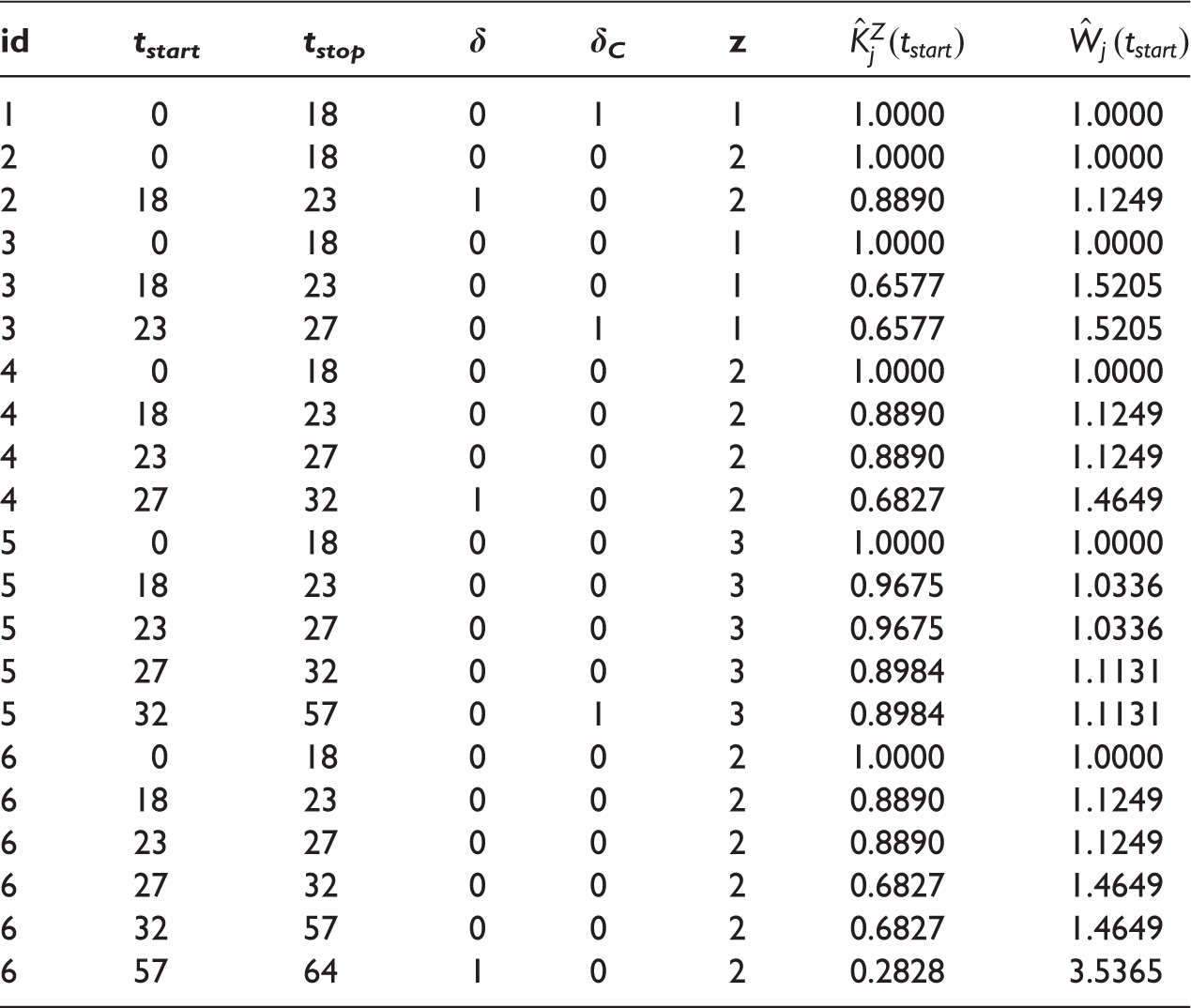
2.2.3 Step 3: Compute IPCW weights

The weights for each subject j are computed as ${\hat{W}}_{j} (t) = 1 / {\hat{K}}_{j}^{Z} (t)$ , which is inversely proportional to the estimated probability of remaining uncensored until time t. The estimated IPCW weights for the toy example are given in Table 2.

At the end of the study time, when most subjects have experienced the event or have been censored, the probabilities of remaining uncensored become very small. Hence, the IPCW estimator weights will become large and unstable. Weights can be stabilized by dividing the marginal probability of remaining uncensored by the estimated probability of remaining uncensored ( ${\hat{K}}_{j}^{0} (t) / {\hat{K}}_{j}^{Z} (t)$ ).

2.2.4 Step 4: Estimate the IPCW version of the survival curve

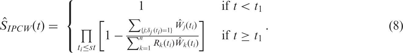
In Steps 1–3, it was described how to compute weights for all subjects at risk at each observed time point. By weighting the subjects, a model for time to event in the absence of censoring can be fitted. KM estimator for time to event is adjusted to include the weighted subjects as follows

{\hat{S}}_{IPCW} (t) = {\begin{matrix} 1 & if t < t_{1} \\ \underset{t_{i} \leq s t}{Π} [1 - \frac{\sum_{{j; δ_{j} (t_{i}) = 1}} {\hat{W}}_{j} (t_{i})}{\sum_{k = 1}^{n} R_{k} (t_{i}) {\hat{W}}_{k} (t_{i})}] & if t \geq t_{1} \end{matrix} .

(8)

The numerator

\sum_{{j; δ_{j} (t_{i}) = 1}} {\hat{W}}_{j} (t_{i})

is the sum of weights of all subjects who experience the event at time point t_i. It represents the estimated number of events that would have occurred at t_i in the absence of censoring. It can be compared to the term d_i in equation (1). The denominator

\sum_{k = 1}^{n} R_{k} (t_{i}) {\hat{W}}_{k} (t_{i})

is the sum over weights of all subjects who are at risk at t_i. It represents the estimated number of subjects at risk at t_i in the absence of censoring, as Y_i in equation (1). Note that in case the stabilized weights are implemented, the numerator

{\hat{K}}_{j}^{0} (t)

is cancelled out in equation (8), i.e. stabilized and unstabilized weights result in the same survival probability estimates.

Survival probabilities estimated with IPCW (

{\hat{S}}_{IPCW} (t)

) for the toy example are compared to the survival probabilities estimated with standard KM (

\hat{S} (t)

) in Table 3. The difference between these probabilities is very small because there are only few subjects and no dependent censoring was induced in the data.

Table 3.

Survival probabilities for the toy data set estimated with standard Kaplan–Meier ( $\hat{S} (t)$ ), and the IPCW estimator version ( ${\hat{S}}_{IPCW} (t)$ ).

t	$\hat{S} (t)$	${\hat{S}}_{IPCW} (t)$
18	1.000	1.000
23	0.800	0.810
27	0.800	0.810
32	0.533	0.517
57	0.533	0.517
64	0.000	0.000

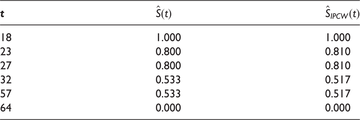
Figure 1 showed the poor performance of traditional KM in the presence of dependent censoring in data. To correct for dependent censoring, the IPCW estimator version of the survival curve was estimated on the same data set (denoted by KM_IPCW). The results are shown in Figure 2 where the classical KM is plotted along with KM_IPCW and the real survival curve. From this figure, we can conclude that IPCW reduced the bias caused by dependent censoring. More simulation results will be shown in section 4.

Figure 2.

Real survival curve and its Kaplan–Meier estimates with (KM_IPCW) and without (KM) implementing IPCW.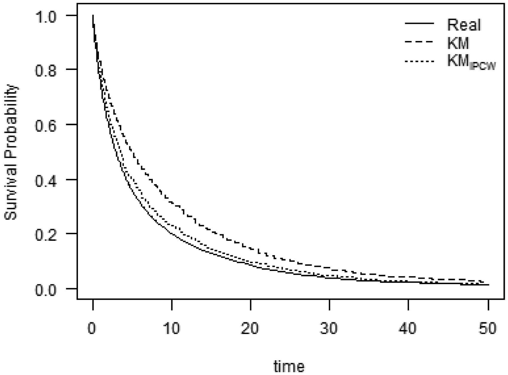

3 Application

3.1 Routine outcome monitoring data

IPCW is applied to a data set from the Department of Psychiatry at the LUMC and Rivierduinen, a local healthcare provider, in The Netherlands. All patients diagnosed with Diagnostic Statistical Manual – fourth edition – text revision (DSM-IV-TR) mood and/or anxiety disorder and with suicidal ideation were included in the data set. Suicidal ideation was defined as a score of 2 or higher on item 10 of the Montgomery–Åsberg Depression Rating Scale (MADRS⁹). Data were collected through a procedure known as routine outcome monitoring (ROM)¹⁰ used to gather information concerning treatment progress by repeatedly measuring symptom severity. The goal is to diagnose patients and to inform clinicians and patients about the treatment progress. The data set was used to identify baseline predictors for remission of suicidal ideation. Remission of suicidal ideation was defined as a score below 2 on item 10 of the MADRS. Socio-demographic variables, functional and clinical scores on several other psychometric instruments were considered as possible predictors for remission. All patients were followed from diagnosis until remission or loss to follow-up, with a maximum of two years.

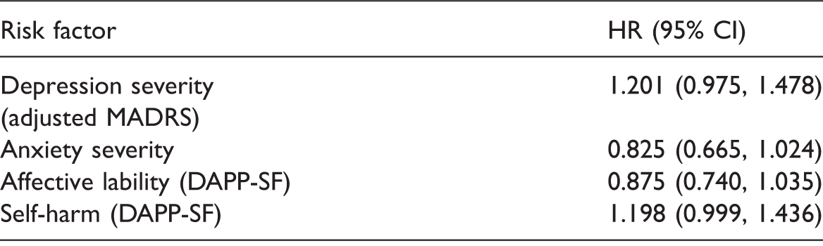
Standard survival analysis was performed on the data set of 769 depressed and/or anxious patients with suicidal ideation at baseline. Baseline scores were determined by the Dutch dimensional assessment of personality pathology-short form (DAPP-SF) and the 36-item short form health survey (SF-36). DAPP-SF is a short form of the dimensional assessment of personality pathology-basic questionnaire (DAPP-BQ) used for the assessment of personality pathology. SF-36 is a set of quality-of-life measures. To detect baseline covariates with a significant effect on remission of suicidal ideation, the Cox model was fitted. Table 4 shows the hazard ratios and the corresponding 95% confidence intervals.

Table 4.

Hazard ratios for remission of suicidal ideation.

Risk factor	HR (95% CI)
Education level
Low	1
High	1.169 (0.990, 1.380)
Depression severity	0.841 (0.774, 0.913)
(adjusted MADRS)
Self-harm (DAPP-SF)	0.773 (0.711, 0.841)
General health (SF-36)	0.913 (0.841, 0.992)

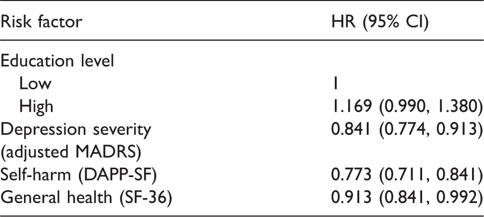
MADRS: Montgomery–Åsberg depression rating scale; DAPP-SF: Dutch dimensional assessment of personality pathology-short form.

Covariate self-harm is the most significant covariate. To compare survival curves for patients with different levels of self-harm, clinicians defined three groups for this variable: low, medium, and high. In Figure 3, the estimated KM curves are shown for these three groups. Recall that the event of interest is remission; hence, low survival probability is favorable for patients, since it indicates a high probability of remission.

Figure 3.

Kaplan–Meier curves for remission from suicidal ideation.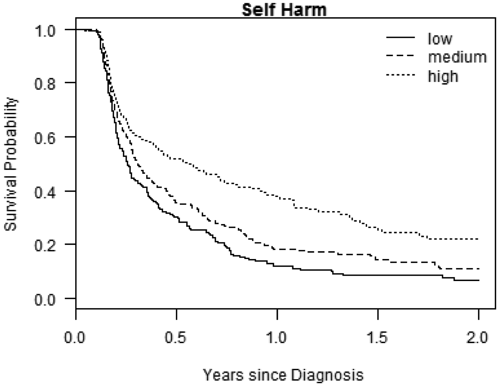

3.2 Correcting for dependent censoring in ROM data

In this study, researchers were only interested in time to remission within the first two years after diagnosis. Therefore, each patient who did not experience the event of interest within two years was censored at two years, as is shown in Figure 4. This is called administrative censoring and was applied to all patients who were still at risk two years after baseline measurements (5.2% of the included patients). Censoring at two years was independent of patient characteristics. Many patients in the ROM data set (18.2%) were censored during the first two years after baseline measurements. These patients are represented by the steps in the inverse KM curve for time to censoring (Figure 4) during the first two years.

Figure 4.

Inverse Kaplan–Meier curve for time to censoring representing the probability of being censored at each time point since diagnosis, given that the subject was not censored until that time point.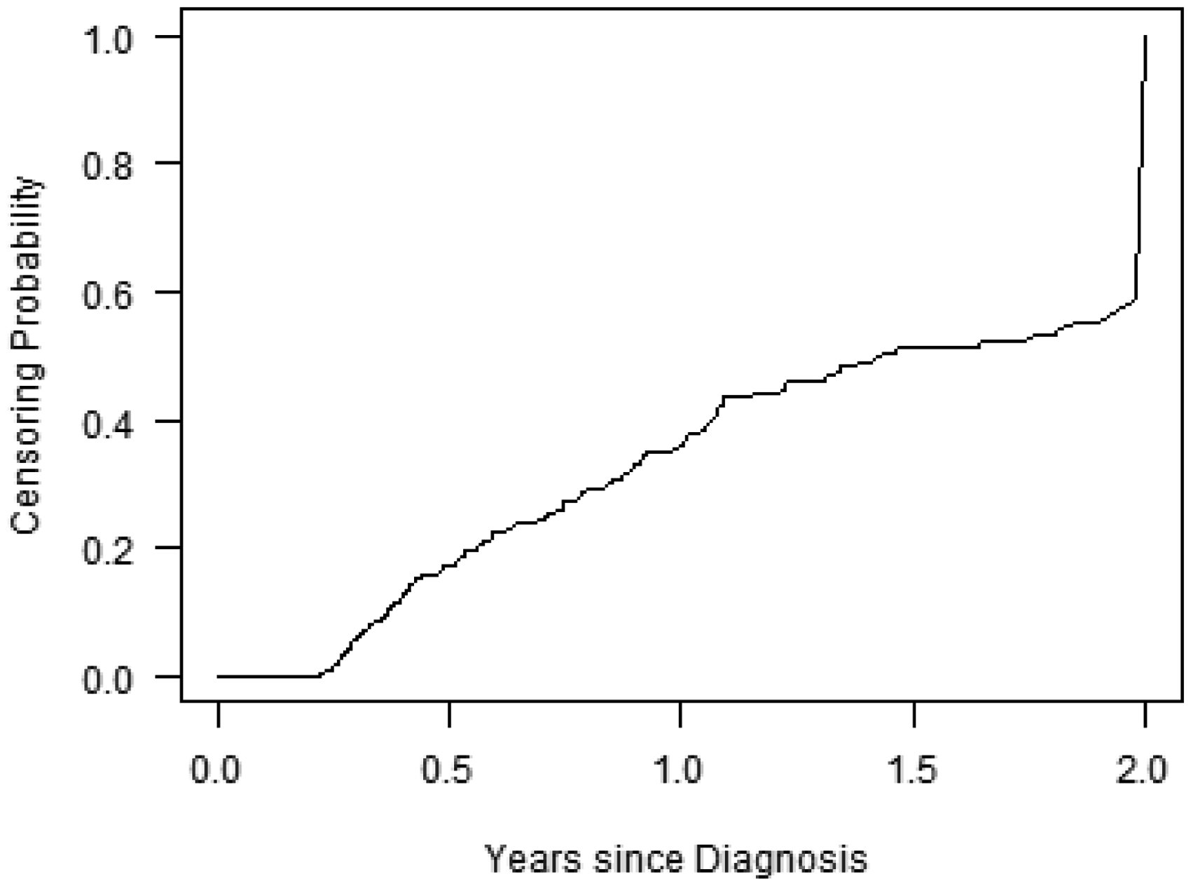

Clinicians believe that patients’ withdrawal is likely to be related to their health status. As ROM sessions took place approximately every three months and a final measurement session was not obligatory, it is conceivable that patients who achieved remission, and therefore ended the treatment, did not have a final ROM measurement reflecting their improvement. This suggests a dependence between time to event and time to censoring through health status, i.e. presence of dependent censoring. If true, this would result in overestimation of survival probabilities, since patients who are more likely to experience the event (remission) are also more likely to be censored. Therefore, less events will be observed, and the survival probabilities will be overestimated. IPCW was applied to this data set to try to correct for dependent censoring. Unfortunately, there is no covariate that directly represents the health status of patients. Instead, several covariates related to health status were used to fit the censoring model. In this example, we rely on the assumption that patients who do not return for a ROM assessment due to their remission were close to remission on their last assessment. If this assumption does not hold, it is impossible to observe whether patients that are almost in remission are more likely to be censored than patients with a bad health status.

Since the administrative censoring is independent of patient’s characteristics, patients who were censored at two years after diagnosis should not be included in the Cox model for the censoring mechanism. Therefore, the IPCW method described in this section is based on a censoring model for time to non-administrative censoring.

In the censoring model, socio-demographic variables and baseline scores considered to be possible predictors for remission were included. In Table 5, hazard ratio’s for time to censoring and their corresponding 95% confidence intervals are shown.

Table 5.

Cox model for time to censoring.

Risk factor	HR (95% CI)
Depression severity	1.201 (0.975, 1.478)
(adjusted MADRS)
Anxiety severity	0.825 (0.665, 1.024)
Affective lability (DAPP-SF)	0.875 (0.740, 1.035)
Self-harm (DAPP-SF)	1.198 (0.999, 1.436)

MADRS: Montgomery–Åsberg depression rating scale; DAPP-SF: Dutch dimensional assessment of personality pathology-short form.

The censoring model to be fitted in step 1 of the IPCW algorithm includes all covariates given in Table 5, and those that are significantly associated to time to event (Table 4). This censoring model was used to estimate the conditional probabilities of remaining uncensored (step 2), and IPCW estimator weights (step 3). The resulting IPCW survival curve (step 4) is almost identical to the original KM curve estimated without applying IPCW estimator (not shown). This suggests that the dependent censoring has hardly any influence on the estimated survival probabilities at population level. However, by looking at the individual level difference between the prediction for the model with and without IPCW $| {\hat{β}}_{X}^{IPCW} Z_{j} - {\hat{β}}_{X}^{0} Z_{j} |$ , some difference between the survival curves estimated with (KM_IPCW) and without IPCW weights (KM) can be found. Results are shown in Figure 5. Hence, IPCW does have an impact on individual level. As Figure 5 shows, KM estimator overestimates the survival probabilities and this result confirms clinicians’ experience.

Figure 5.

Survival curves estimated with and without the IPCW method for the subject for whom 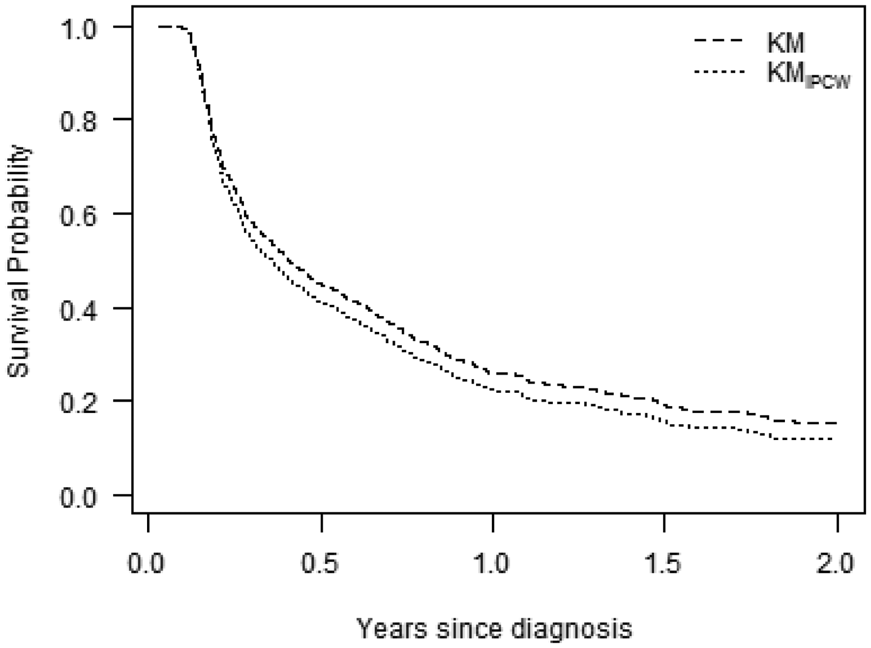$| {\hat{β}}_{X}^{IPCW} Z_{j} - {\hat{β}}_{X}^{0} Z_{j} |$ is the largest.

4 Simulation study

A simulation study was performed to investigate the behavior of IPCW under different scenarios.¹¹ In the simulation process, different sample sizes, strengths of the censoring model, and percentages of censored individuals were chosen. In this section, all steps in the simulation process are illustrated and part of the results coming from a large simulation study is discussed.

4.1 Steps in the simulations process

Step 1

For each subject j, $j = 1, \dots, n$ , generate a continuous variable Z₁ from a standard normal distribution and generate a categorical variable Z₂ from a Bernoulli distribution with p = 0.5.

Step 2

Determine the hazards for event and censoring for each individual in the data set. Hazards depend on covariates Z₁ and Z₂:

h_{X} (t | Z) = h_{0_{X}} (t) exp (β^{t} Z),

(9)

h_{C} (t | Z) = h_{0_{C}} (t) exp (φ^{t} Z) .

(10)

Step 3

Sample the event times x_j and censoring times c_j from an exponential distribution, with rates $h_{X} (t | Z_{j})$ and $h_{C} (t | Z_{j})$ , respectively.

Step 4

For each individual compute the observed time point $t_{j} = min (x_{j}, c_{j})$ , and the corresponding event indicator δ_j.

Step 5

Estimate the true survival curve (KM on x_j), the standard KM result (KM on $(t_{j}, δ_{j})$ ), and the IPCW estimator survival estimates (IPCW on $(t_{j}, δ_{j})$ ).

All details concerning the method developed to generate survival data with dependent censoring and different scenarios are outlined in Supplementary Material B.

4.2 Varying the sample size

To investigate the effect of sample size n on IPCW results, simulations were performed with different numbers of subjects. Three different sample sizes n equal to 100, 250, and 500 were chosen. The other variables, like strength of the censoring model ( $φ = (1.5, 5)$ ), censoring percentage (35%), and strength of the time to event model ( $β = (0.5, 1.5)$ ) remained constant. Results are illustrated in Figure 6. As expected, the survival curve estimated by employing IPCW gets closer to the real survival curve for increasing n, while KM estimator’s performance does not change when more subjects are observed. The improvement of the IPCW result is due to more precise regression coefficient estimates for the censoring model based on large sample sizes, which leads to more accurate IPCW weights, hence in better estimation outcome. As shown in Figure 6(a), IPCW always gives better results than standard KM, even in case of a small sample size.

Figure 6.

True survival probabilities (Real) and the survival curves estimated with standard Kaplan–Meier (KM) and IPCW (KM_IPCW) corresponding to different sample sizes, n equal to 100 (figure a), 250 (figure b), and 500 (figure c).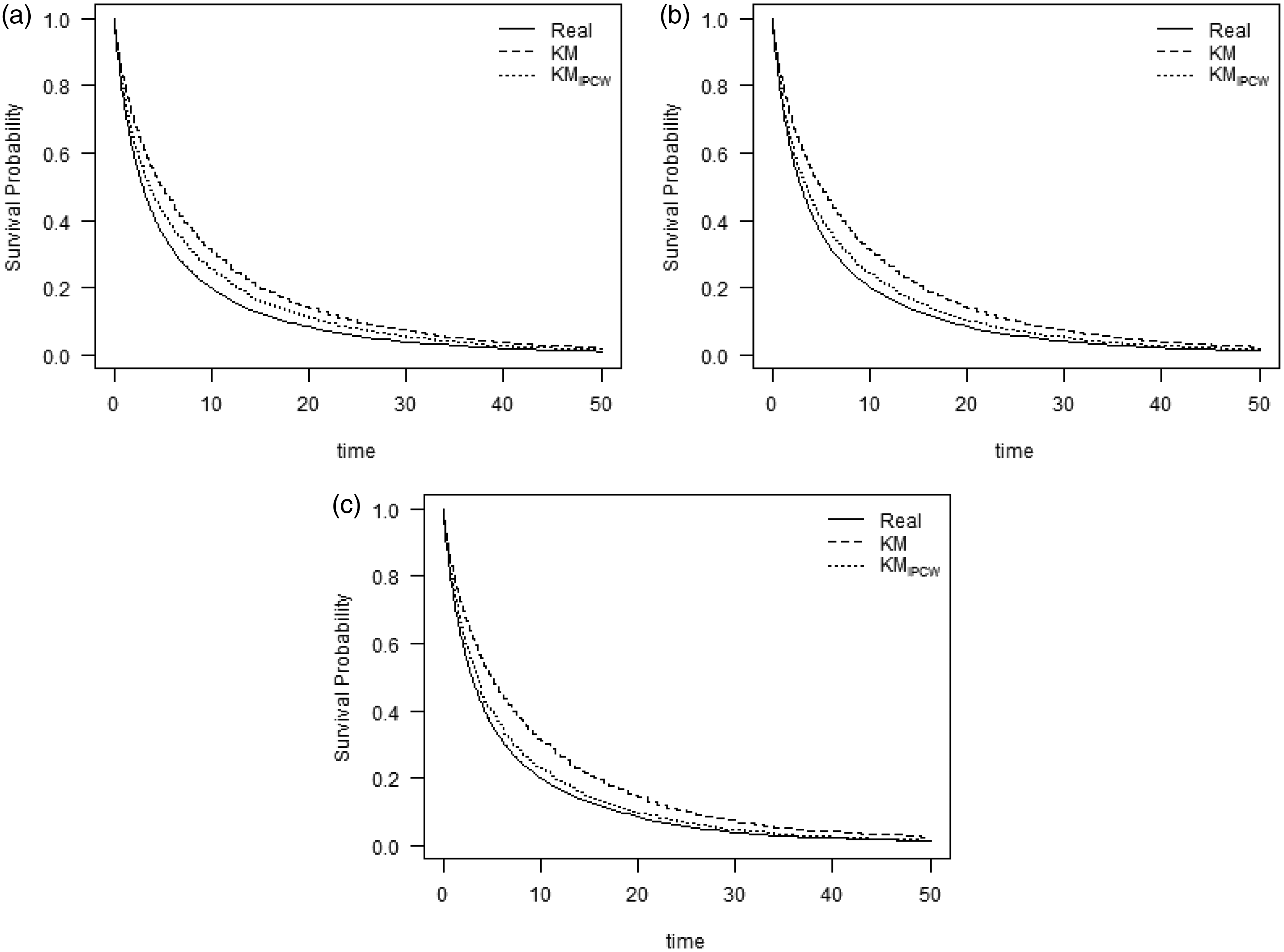

4.3 Varying the strength of the censoring model

The strength of the censoring model is defined by the parameter $φ = (φ_{1}, φ_{2})$ , where $φ_{1}$ is the regression coefficient for Z₁, and $φ_{2}$ indicates the effect of the categorical variable Z₂. For larger absolute values of $φ_{1}$ and $φ_{2}$ , the dependence between the censoring mechanism and the covariates becomes stronger. Values of φ equal to (1.5, 5) and (0.75, 2) correspond to strong and weak censoring mechanisms, respectively. Values of φ equal to (0, 0) means absence of dependent censoring.

In Figure 7, results corresponding to the different values of the censoring mechanism are shown. In these scenarios β is equal to (0.5, 1.5), the sample size n is equal to 100 and 35% of the subjects were censored. The two covariates Z₁ and Z₂ were generated from a standard normal distribution and a Bernoulli distribution, respectively. The first may, for example, represent the ages of subjects in the study and the second one may represent gender (e.g. 0 = male and 1 = female). In this case, the choice of $φ = (1.5, 5)$ for the strong censoring mechanism indicates that $exp (5)$ is the risk for women to experience the event compared to men. Furthermore, older individuals have higher censoring hazards compared to younger individuals. In the presence of weak censoring, the hazard ratio between women and men is equal to $exp (2)$ , and the difference between the hazards of young and old subjects is also smaller. Hence, when weak censoring is present in the data, covariates have a smaller effect on the hazard, i.e. the censoring effect is smaller than in the former situation (strong censoring mechanism).

Figure 7.

True survival probabilities (Real) and the survival curves estimated with standard Kaplan–Meier (KM) and IPCW (KM_IPCW) corresponding to different parameters φ in the censoring model. The combinations used are 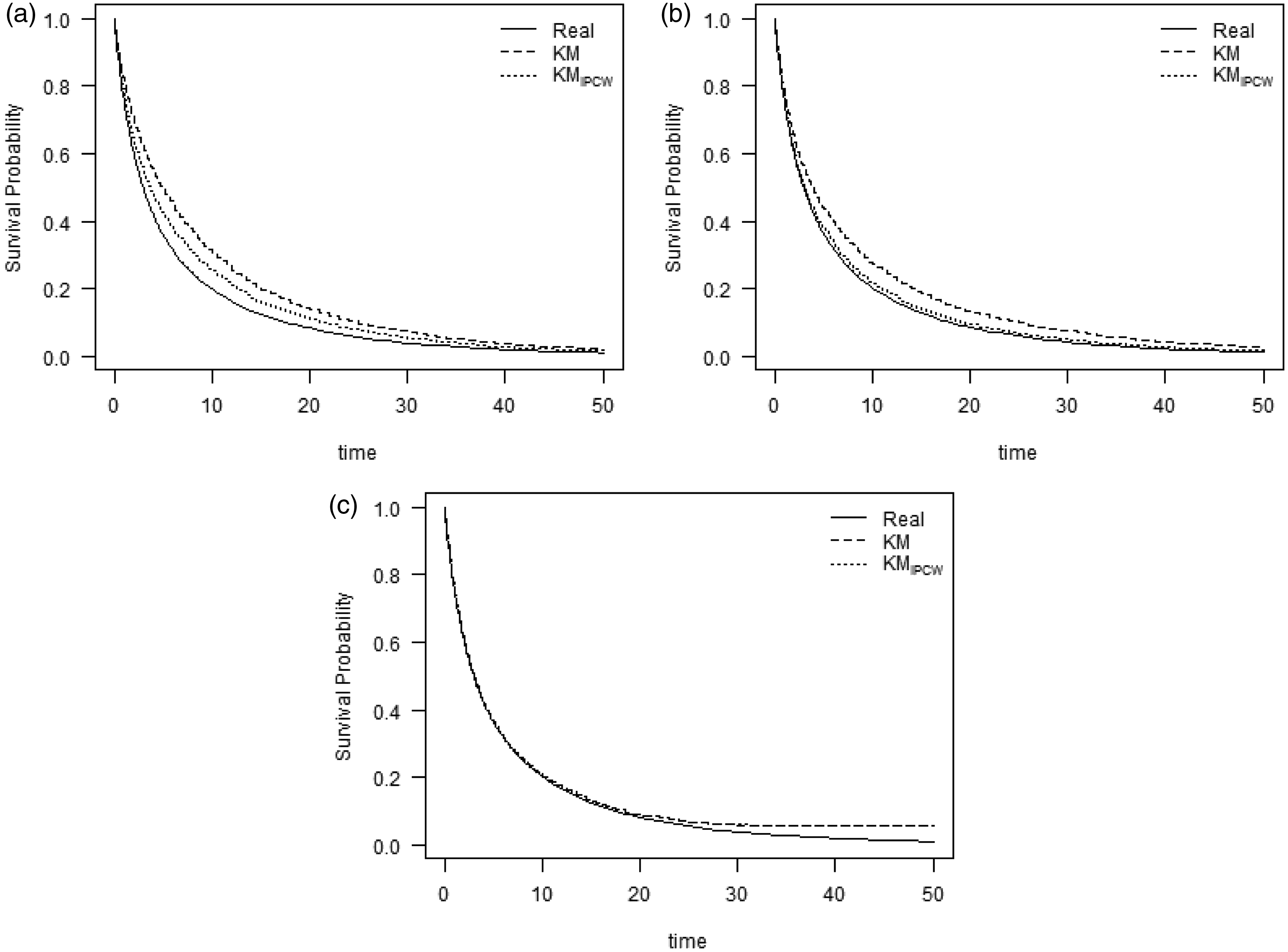$φ = (1.5, 5)$ with $h_{0_{C}} = 0.00557$ (figure a), $φ = (0.75, 2)$ with $h_{0_{C}} = 0.041$ (figure b), and $φ = (0, 0)$ with $h_{0_{C}} = 0.102$ (figure c).

When considering these strong and weak censoring models, subjects who have a higher probability of experiencing the event also have a higher chance of being censored. Therefore, less events are observed and survival probabilities are overestimated by both standard KM and IPCW (Figure 7(b) and 7(a)). The stronger the censoring mechanism, the worse the fit for both methods. However, IPCW estimator is less biased than standard KM in both cases. In the absence of dependent censoring ( $φ = (0, 0)$ ), both IPCW and standard KM give accurate results (Figure 7(c)). This suggests that the IPCW method gives good estimates even in case dependent censoring is not present.

4.4 Varying the percentage of censored subjects

Varying the percentage of censored subjects, while keeping the censoring model constant ( $φ = (1.5, 5)$ ), can be done by changing the baseline probability of being censored ( $h_{0_{C}}$ ). Simulations were performed to find $h_{0_{C}}$ corresponding with censoring percentages equal to 35%, 50%, or 65%. In each simulation, $β = (0.5, 1.5)$ and sample size is equal to 100. Results in Figure 8 show that the performance of both methods becomes worse with increasing censoring percentage. This was expected, since it is well known that the precision of the estimate declines with increasing censoring percentage.

Figure 8.

True survival probabilities (Real) and the survival curves estimated with standard Kaplan–Meier (KM) and IPCW (KM_IPCW) corresponding to different censoring percentages, namely 35% (figure a), 50% (figure b), and 65% (figure c).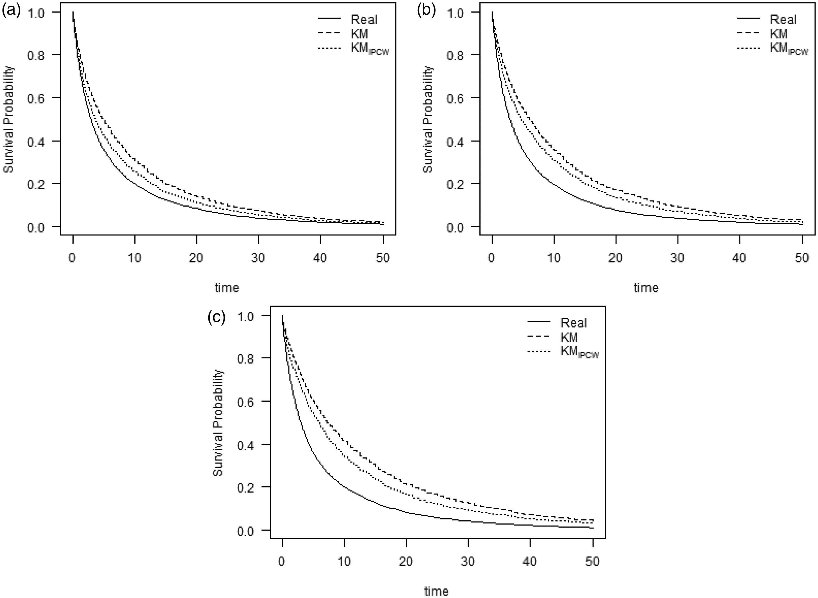

5 Discussion

Standard survival analysis techniques assume independence between time to event and censoring. This assumption is violated when covariates are associated to both event and censoring time. In case of dependent censoring, traditional methods, like the KM estimator, may give biased estimates for survival probabilities. IPCW can be used in these situations; this method corrects for censored subjects by giving extra weight to those who remain at risk, and assigning more weight to subjects that are more similar to the censored one.

IPCW was applied to a clinical data set where patients suffer from suicidal ideation. Time to remission was the event of interest. The IPCW method did not seem to have an effect on estimated survival curves at population level, but it did have an impact on individual level. This result does not necessarily imply that dependent censoring is not present in the data. There could be unmeasured covariates that influence both time to event and time to censoring, or there could be a mechanism that causes event and censoring times to be directly dependent, i.e. not only through covariates. In these cases, the censoring model estimated with IPCW does not fully describe the censoring mechanism. Therefore, the IPCW results do not completely correct for the censoring mechanism.

A simulation study was carried out to study the performance of IPCW in case of dependent censoring. Dependent censoring was induced in the generated survival data by simulating two time independent covariates that influence both time to event and time to censoring. Several different scenarios were generated by varying the sample size, the strength of the censoring mechanism, and the percentage of censored subjects. The simulation study showed that in each scenario, IPCW performs better than the standard survival technique. The better the fit for the censoring model, the more accurate the IPCW result. In this simulation study, event and censoring times were generated from an exponential distribution, i.e. constant hazard rates were assumed for both models. In practice, hazards may not be constant, but may vary over time. Therefore, an additional simulation study was done where hazards are not constant. Both time to event and censoring time were generated from Gompertz distribution.¹² Also in this situation, results (not shown in this article) showed that IPCW gives better survival estimates than the KM estimator.

The corrected group prognosis method (CGP)¹³ might be used as an alternative to IPCW in case of dependent censoring. Here, the Cox model is fit to the whole data set. Then, survival curves, conditional on the observed covariates, are estimated for each subject in the data set. The marginal survival curve is then obtained by averaging over the covariate-specific curves. Since dependent censoring does not cause bias in the Cox model, this method will give an unbiased result for the marginal survival curve. The simulation study described in this article was repeated to compare the performance of CGP with the performance of IPCW. Simulation results suggest that both methods perform well in case of dependent censoring. However, while IPCW can deal also with time varying covariates (covariates which value may change over time), CGP cannot. In these situations, CGP will not perform well, since it does not incorporate time varying covariates in the estimations of individual survival curves for each subject. Time varying covariates can be included in the Cox model for time to censoring, and can therefore be incorporated in the IPCW methodology.

In the analysis of survival data, attention is mainly given to the survival times and prognostic factors, but almost no attention is given to the censoring mechanism. If the probability of being censored is not the same for each individual at risk, standard survival analysis techniques may give biased results. Further investigation on the censoring mechanism may be needed and IPCW that adjusts for dependent censoring can be applied.

Footnotes

Acknowledgement

The Department of Psychiatry of Leiden University Medical Center (LUMC) in The Netherlands is gratefully acknowledged for providing the data.

Declaration of conflicting interests

The author(s) declared no potential conflicts of interest with respect to the research, authorship, and/or publication of this article.

Funding

The author(s) received no financial support for the research, authorship, and/or publication of this article.

Supplement Material

Supplementary material is available for this article online.

References

Robins

Rotnitzky

Recovery of information and adjustment for dependent censoring using surrogate markers. In: Jewell

Dietz

Farewell

(eds). AIDS Epidemiology, Boston: Birkhäuser, 1992, pp. 297–331.

Robins JM. Information recovery and bias adjustment in proportional hazards regression analysis of randomized trials using surrogate markers. In: Proceedings of the biopharmaceutical section, Virginia: American Statistical Association, 1993, pp.24–33.

Robins

Finkelstein

. Correcting for noncompliance and dependent censoring in an aids clinical trial with inverse probability of censoring weighted (IPCW) log-rank tests. Biometrics 2000; 56: 779–788.

Kaplan

Meier

. Nonparametric estimation from incomplete observations. J Am Stat Assoc 1958; 53: 457–481.

Kleinbaum

Klein

. Survival analysis: a self-learning text (statistics for biology and health), 3rd ed. New York: Springer, 2012.

R Development Core Team. R: A language and environment for statistical computing. Vienna Austria: R Foundation for Statistical Computing, 2008. ISBN 3-900051-07-0. http://www.R-project.org.

Therneau TM. A package for survival analysis in S, 2013. R package version 2.37-4, http://CRAN.R-project.org/package=survival (accessed 13 January 2016).

Therneau

Grambsch

. Modeling survival data: extending the Cox model, New York, NY: Springer, 2000.

Montgomery

Åsberg

. A new depression scale designed to be sensitive to change. Br J Psychiat 1979; 134: 382–389.

10.

de Beurs E, den Hollander-Gijsman ME, van Rood YR, et al. Routine outcome monitoring in the Netherlands: practical experiences with a web-based strategy for the assessment of treatment outcome in clinical practice. Clin Psychol Psychother 2011; 18(1): 1–12.

11.

Mooney

. Monte Carlo Simulation (Sage University Paper series on Quantitative Applications in the Social Sciences, series no. 07-116), Thousand Oaks, CA: Sage, 1997.

12.

Bender

Augustin

Blettner

. Generating survival times to simulate Cox proportional hazards models. Stat Med 2005; 24(11): 1713–1723.

13.

Chang

Gelman

Pagano

. Corrected group prognostic curves and summary statistics. J Chronic Dis 1982; 35: 669–674.

Supplementary Material

Please find the following supplemental material available below.

For Open Access articles published under a Creative Commons License, all supplemental material carries the same license as the article it is associated with.

For non-Open Access articles published, all supplemental material carries a non-exclusive license, and permission requests for re-use of supplemental material or any part of supplemental material shall be sent directly to the copyright owner as specified in the copyright notice associated with the article.

0.00 MB

0.28 MB