Statistical approaches to account for missing values in accelerometer data: Applications to modeling physical activity

Abstract

Physical inactivity is a recognized risk factor for many chronic diseases. Accelerometers are increasingly used as an objective means to measure daily physical activity. One challenge in using these devices is missing data due to device nonwear. We used a well-characterized cohort of 333 overweight postmenopausal breast cancer survivors to examine missing data patterns of accelerometer outputs over the day. Based on these observed missingness patterns, we created psuedo-simulated datasets with realistic missing data patterns. We developed statistical methods to design imputation and variance weighting algorithms to account for missing data effects when fitting regression models. Bias and precision of each method were evaluated and compared. Our results indicated that not accounting for missing data in the analysis yielded unstable estimates in the regression analysis. Incorporating variance weights and/or subject-level imputation improved precision by >50%, compared to ignoring missing data. We recommend that these simple easy-to-implement statistical tools be used to improve analysis of accelerometer data.

Keywords

Accelerometer data missing data physical activity weighted regression linear mixed effects model

1 Introduction

Physical inactivity and sedentary behavior are recognized risk factors for many chronic diseases,^1–4 driving research on levels of physical activity needed to maintain a healthy lifestyle and prevent disease. Accelerometers are objective means to measure duration and intensity of daily physical activity, and may be less prone to the biases associated with self-report.^5,6 Traditional protocols for hip-worn accelerometers instruct participants to wear the device for at least five days during waking hours.⁷ Unfortunately missing data, due to participants removing their accelerometer for varying and undocumented reasons, lead to nonrandom bias, which in turn often results in inaccurate assessments of physical activity. These missing data and attending biases present a major obstacle to the interpretation of accelerometer-based research.

Previous studies have highlighted the error caused by inconsistencies in the number of wear days across participants.⁸ In addition, errors due to variations in the amount of wear time each day have been outlined, with substantial bias noted when daily wear time was less than 12 h.^9,10 However, including only days with ≥ 12 h of device wear would result in researchers being forced to discard a large amount of otherwise usable participant data. To combat these potential biases and yet make optimal use of available information, the majority of accelerometer studies include only data that meets a minimum required number of days (≥ 3–5 days^11,12) and time per day (ranging 6–10 h/day),^12–14 and then account for wear time variation by either (a) using imputation methods,^15–17 (b) normalizing activity measures by wear time,^14,18,19 and/or (c) adjusting for wear time in regression models.^20,21 In addition, a few use Bayesian techniques to incorporate individuals with as little as one day of valid wear time.^22,23 Thus, there is as yet no consensus regarding the optimal analytic method for accounting for nonwear time, with a variety of methods in use, making it difficult to compare results across studies.

In this article, we focused on a regression modeling framework, and aimed to develop and evaluate statistical methods to standardize analysis and accurately estimate regression parameters of interest despite the presence of missing data due to nonwear. A primary objective was to develop methods that would be easy to implement using standard software and thus accessible to the physical activity research community. We implemented a pseudosimulation approach, whereby realistic missing data patterns were simulated. We used baseline data from a cohort of postmenopausal breast cancer survivors to create the pseudosimulated datasets. Next, a variety of statistical methods to account for variability in device wear time were applied to these simulated data; bias and precision of these methods were compared. The outline of this article is as follows: in Section 2, we provide details on demographics and accelerometer measures available for our study sample. In Sections 3 and 4, we specify the objectives of our analysis, what we consider “complete” profiles for the purposes of the simulations, and the regression model and parameters of interest. Section 5 covers our algorithm for simulating missing data patterns from complete profiles. In Sections 6 to 9 we propose three analytic methods to account for missing values in accelerometry data, evaluate the performances of these methods, and discuss a Poisson framework to justify the relative success of one of our proposed methods. We conclude (Section 10) with a discussion of strengths and weaknesses of our approach and some recommendations for use of the methods.

2 Study sample

Our study cohort comprised of 333 overweight postmenopausal breast cancer survivors participating in a weight-loss intervention trial.²⁴ Participants were on average 63 (SD = 6.9) years with mean BMI 31.1 (SD = 4.9) at study entry; 51% had college degree or higher, 48% had Stage I, 35% Stage II, and 17% Stage III breast cancer.

Objective physical activity in our study was assessed via the GT3X Actigraph (ActiGraph, LLC; Pensacola, FL), which is a triaxial lightweight accelerometer approximately 2 × 2 × 1 in size. The Actigraph GT3X + monitor was set to collect acceleration data at 30 Hz. The ActiLife program applied a band-pass filter to remove nonhuman acceleration signal from the data and then summarized the signal to counts per minute using a proprietary algorithm.²⁵ The magnitude of the count is related to intensity of the activity.²⁵ The device has been validated and calibrated for use in both controlled and field conditions.²⁵ Participants were provided with written protocols for best positioning of the device and instructed to wear it on the hip for seven days during all waking hours, except for when in contact with water. Nonwear time was identified via predefined algorithms of consecutive zero counts using standard protocols²⁶ and labeled as missing data.

Our sample had a total of 2814 days of accelerometer data, with the number of days per participant ranging from 2 to 21. Median wear time per day was 816 min (25%-ile = 725 min, 75%-ile = 895 min).

3 Study objectives and general strategy

A major objective in behavioral studies is identifying demographic and other factors associated with a behavior of interest (e.g. dietary intake or physical activity level). Hence our primary objective in the current study was to fit regression models to identify factors associated with physical activity level.

For the first set of analyses, we used physical activity volume, i.e. total accelerometer counts per minute, as our measure of physical activity. In later sections (Section 8), we consider other measures (e.g. moderate-to-vigorous activity (MVPA) and sedentary time). Our data comprised accelerometer counts measured on multiple days for each participant. To account for these hierarchical data, we used linear mixed effects models²⁷ with accelerometer count per minute as the nested dependent variable, and age, BMI, depression, and weekend status as independent predictors. Mathematically, our model was specified as

Y_{ij} = α_{i} + A_{i} β_{1} + B_{i} β_{2} + D_{i} β_{3} + W_{ij} β_{4} + ε_{ij}

(1)

Here Y_ij is the average activity count for the jth day of the ith subject. α_i is the random intercept for subject i. A_i is the age for the ith subject. B_i is the BMI for the ith subject. D_i is the depression indicator (1 if depressed, 0 if otherwise) for the ith subject. W_ij is the weekend indicator (1 if it is a weekend day, 0 if otherwise) for the jth day of the ith subject. ε_ij is the random error for the jth day of the ith subject. The parameters, β_k for

k = 1, 2, 3, 4,

are the primary focus of the analysis, representing regression coefficients for age, BMI, depression, and weekend indicator, respectively. Our primary goal was to accurately estimate these coefficients despite the presence of missing data. We emphasize that the particular choice of independent variables is not important to the statistical methods we developed; these variables were chosen to represent “realistic” modeling scenarios, namely mixed data types, comprising of continuous (i.e. age, BMI) and categorical (i.e. depression, weekend status) predictors, with varying strength of association with physical activity, as noted below.

4 Complete profiles and true model parameters

Given our goals, the next step was to identify a “true” dataset from which we could simulate missing data patterns. We defined “complete profiles” as days with 12 or more hours of total wear time.^9,10 Analytic results, in particular those of the previously discussed mixed effects regression model, derived from using only the complete profiles were considered true values.

The set of complete profiles consisted of 328 participants and 2091 days, constituting 75.7% of the total data. The number of days per participant in this set ranged from 1 to 15. We fit the linear mixed model (1) to the complete dataset. Model parameters were estimated as $β_{1} = - 4.600$ (SE=0.833), $β_{2} = - 4.177$ (SE = 1.162), $β_{3} = - 30.930$ (SE = 11.672), and $β_{4} = 8.362$ (SE = 4.654). Moreover, β₁, β₂, and β₃ were significant at the 1% significance level; β₄ was significant at the 10% significance level. These regression estimates will serve as the ground-truth for testing the performance of our proposed methods.

5 Simulating missing data patterns

The next step was to simulate “realistic” missing data patterns from complete profiles. In this section, we first describe the missing data patterns observed in our cohort, and then develop an algorithm to simulate missing data from the complete profiles. Lastly, we discuss how we will apply this algorithm to test the performance of the statistical methods that will be proposed in the next section.

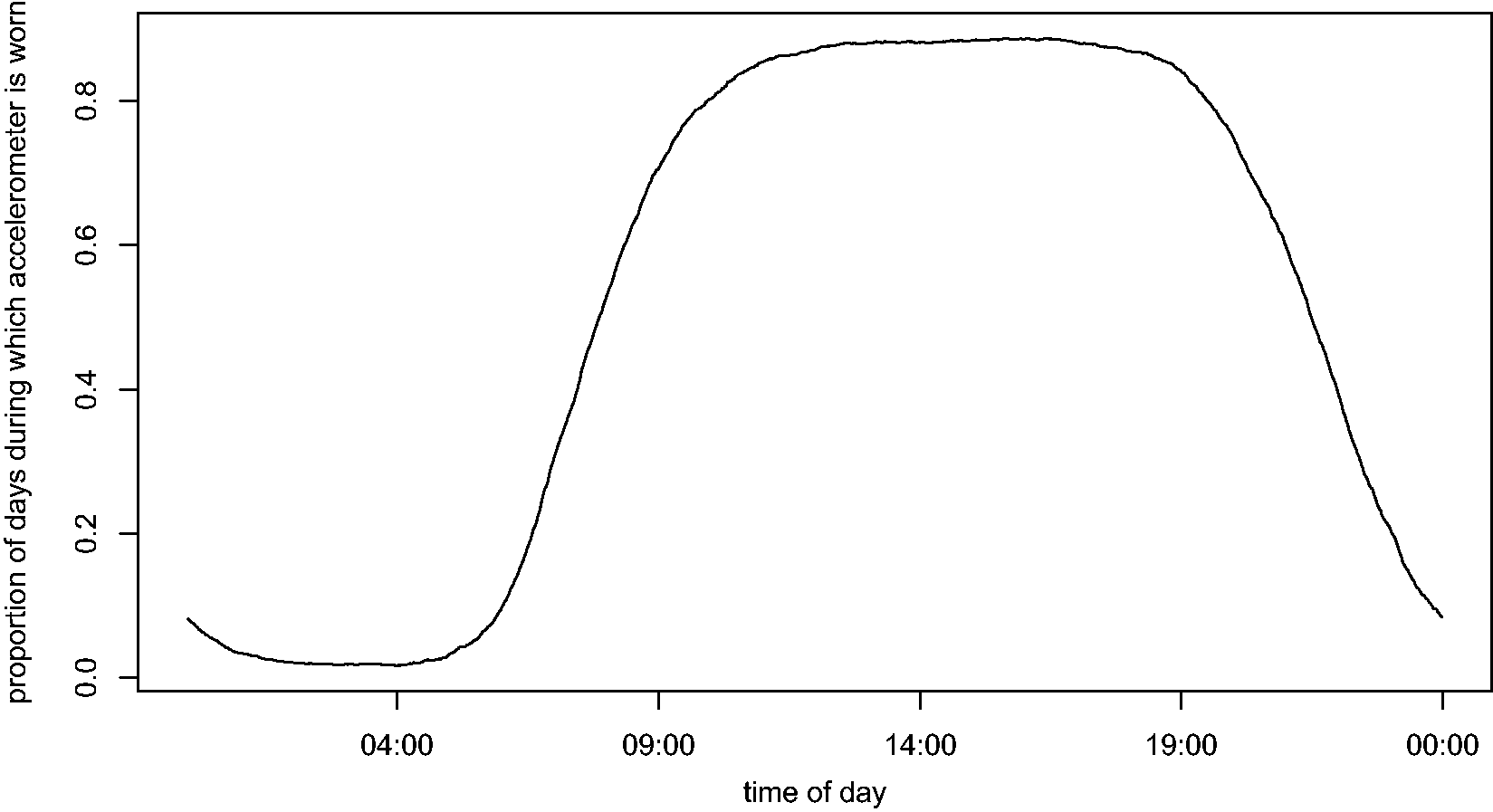
We observed that missing data (Figure 1) tended to be concentrated at the beginning and the end of a day, rather than randomly distributed throughout the day. Among the approximately 25% incomplete (i.e. with < 12 h of recorded activity) daily profiles: 12.2% were missing 50–60% of daily records (of 24 h/1440 min); 2.6% were missing 60–70% of daily records (of 24 h/1440 min); 1.7% were missing 70–80% of daily records (of 24 h/1440 min); 1.8% were missing 80–90% of daily records (of 24 h/1440 min); 6.0% were missing 90–100% of daily records (of 24 h/1440 min). These patterns indicate that generating simulated missing data by randomly excluding minutes of accelerometer wear throughout the day would not reflect actual missing data patterns. Hence, we designed a pairwise comparison simulation algorithm to generate realistic missing data from complete profiles. The goal was to mimic missing data patterns observed in the population, i.e. original full cohort sample. Our simulation scheme consisted of the following steps:

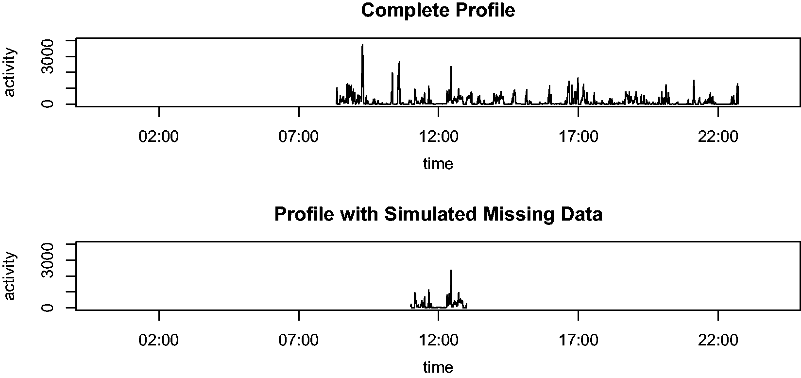
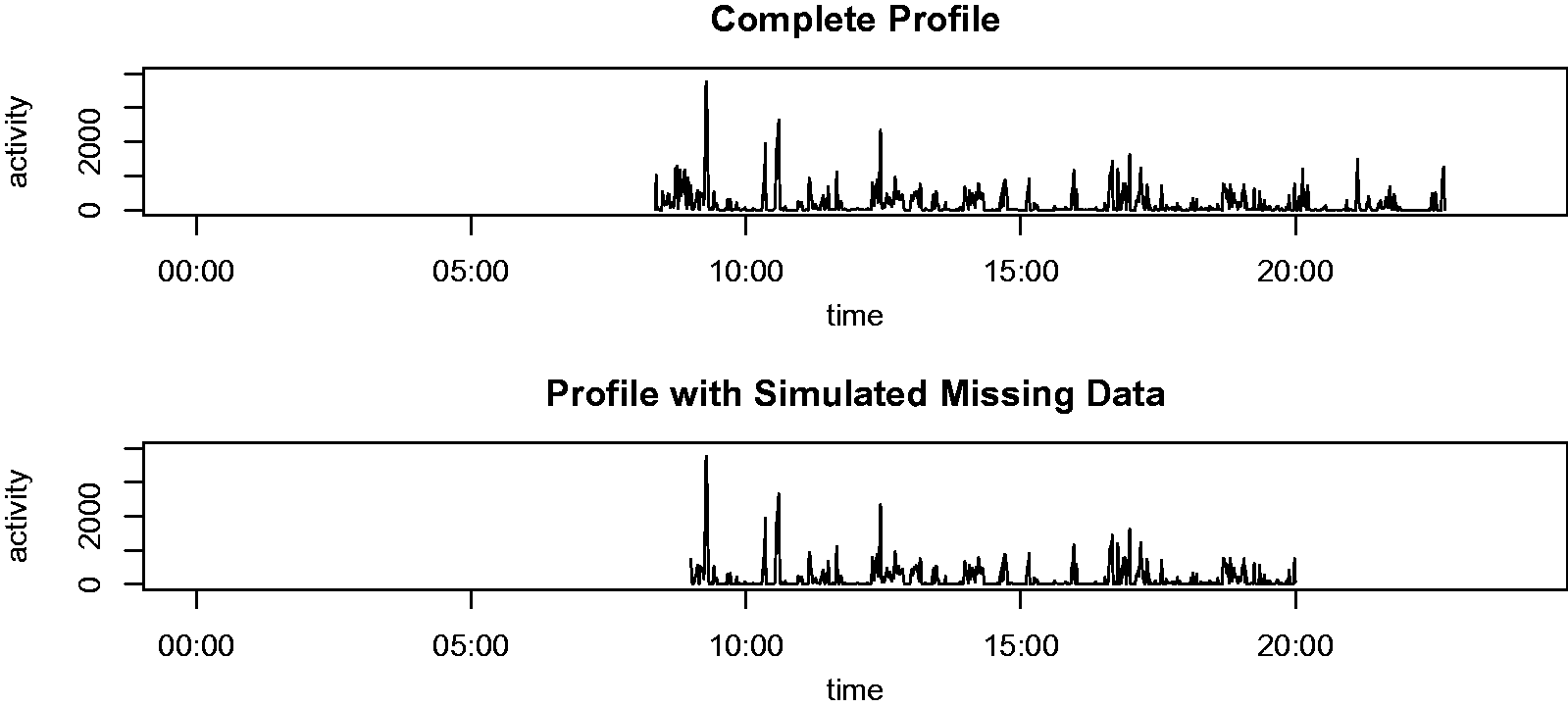
Define five strata of interest: days missing 50–60% data, days missing 60–70% data, days missing 70–80% data, days missing 80–90% data, and days missing 90–100% data.

Following the proportion of each stratum in the population data, randomly sample (without replacement) appropriate numbers of days from the set of complete profiles and assign them to a stratum. For instance, 12.2% of the complete profile set would be assigned to be missing 50–60% of their daily records.

For each complete profile day that is assigned to be in any of the five strata, randomly select a day of the same stratum from the original population dataset and synchronize the missingness of the two days.

We illustrate the algorithm with two examples. Suppose the day sampled from the set of complete profiles had accelerometer counts recorded from 8:20 a.m. to 10:44 p.m. (Figure 2 top profile). Further, according to Step 2, assume that this complete day was assigned to be in the last stratum with 90–100% missing data. Following Step 3, suppose the day of the same stratum chosen from the original dataset only had accelerometer data recorded from 11:00 a.m. to 1:00 p.m. Then our algorithm would “force” the complete profile to retain only its record from 11:00 a.m. to 1:00 p.m. (Figure 2 bottom profile), hence leaving the two days with the same missing data patterns. Suppose in the next simulation, this day (with accelerometer counts recorded from 8:20 a.m. to 10:44 p.m.) is assigned to be in the second stratum with 50–60% missing data. Moreover, the day of the same stratum chosen from the original dataset only had accelerometer data recorded from 9:00 a.m. to 8:00 p.m. Then our algorithm would “force” the complete profile to retain only its record from 9:00 a.m. to 8:00 p.m. (Figure 3 bottom profile), hence leaving the two days with the same missing data patterns.

Figure 1.

Proportion of days during which accelerometer was worn at each time point of the day.

Figure 2.

First example illustrating the missing data simulation algorithm.

Figure 3.

Second example illustrating the missing data simulation algorithm.

With this simulation algorithm in place, our study plan was straightforward. We repeated this simulation algorithm on the complete profiles 100 times, thus creating 100 datasets with missing data patterns reflected in the original population dataset. We applied each of our proposed statistical methods (details below in Section 6) and fitted the mixed effects regression models (1) to each of these 100 simulated datasets. We recorded the regression coefficient estimates, as well as other key information (standard deviation, significance level, etc.) for the parameters of interest for each simulated dataset. These yielded 100 estimates of these parameters, which were used to evaluate, and analytically and graphically compare, the performance of our proposed methods, in terms of mean-squared error, bias, and standard deviation.

6 Statistical methods

We developed and evaluated three different analytic methods that we believed could improve the precision and accuracy of regression estimates in the presence of missing accelerometer data. We describe the rationale and statistical details of these methods below.

6.1 Method 1: Weighted regression

We observed heteroskedasticity in the residuals against the proportion of missing data in a day when fitting the regression model with the raw count data (as illustrated in Figure 4). More specifically, the higher the amount of missing data in a day, the greater the variance of the residuals. Based on this observation, we implemented a weighted linear mixed regression model to account for heteroskedasticity in the residuals. We considered two weighting schemes:

variance ∝ $\frac{1}{1 - τ_{ij}}$ ;

variance ∝ exp( $c [i] \times τ_{ij}$ ).

Here τ_ij refers to the proportion of missing data out of 24 h (or 1440 min) for subject i on day j;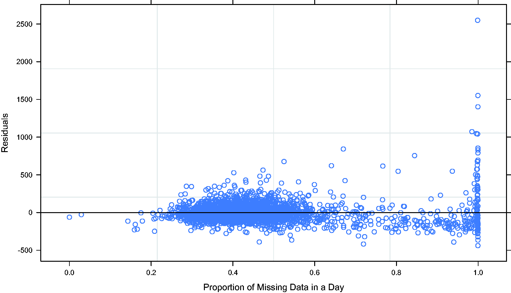

c [i]

denotes a constant c for the ith participant and is determined through a data-driven built-in algorithm in the nlme package in R.²⁸

Figure 4.

Heteroskedasticity in the residuals against the proportion of missing data in a day.

This method is easy to implement with slight modifications to the standard linear mixed regression model. It is also highly efficient in terms of computing time.

6.2 Method 2: “Imputed” daily sum

For the second method, we exploited the availability of multiple daily records and derived imputed estimates of total daily counts, by directly modeling the relationship between individual daily wear time and daily sum of minute-level activity counts. The rationale for this approach was to borrow information from within an individual using her multiple records, as well as, from across other participants’ daily activity profiles, to obtain a more stable and accurate estimate of her own daily average activity. We developed two similar approaches:

Fit a linear mixed regression model with daily sum of activity as the response variable and daily wear time as the predictor variable. Include a random effect for intercept but not slope, thus forcing all subjects to have the same slope $\hat{β}$ . Use this estimated slope to impute missing data: for days with less than 12 h (or 720 min) of accelerometer use, add $\hat{β} \times (720 - wear time)$ to the observed sum of activity counts. This gives a new estimate of 12 h total activity count for all incomplete profiles. Use these imputed activity counts per minute as the outcome in the mixed effect regression model (1).

Generalize the above method by including random effects for both the intercept and the slope for each individual. This gives an estimate ${\hat{β}}_{i}$ for each individual participant. Use this subject-specific slope to impute missing data: for days with less than 12 h of recorded data for individual i, add ${\hat{β}}_{i} \times (720 - wear time)$ to the observed total activity count, and again fit the mixed effects regression model (1).

We also implemented models with a subject-specific slope term alone (i.e. with intercept equal to zero). The results were similar to method ii and are not provided. Similar to the variance-weighting approach, this mixed-effects imputation method is easy to implement, using standard statistical software packages, and is highly efficient in terms of computing time.

6.3 Method 3: K-nearest neighbor (K-NN)

The third method imputed missing data at the minute level even though the dependent variable of interest in our model is at the day level (i.e. daily average activity). In order to impute missing data at the minute level, we used a K-NN method, an approach that originated in the machine learning research field.²⁹ Specifically for each incomplete profile, we would like to find the complete profiles that matched most closely with the nonmissing portion of the incomplete profile. We will then use the minute level information of these complete profiles to impute the missing portion of the incomplete profile. Eventually, after imputation, all daily records would become complete profiles. To evaluate how closely two profiles match each other, we need a measure of distance between physical activity records. In this paper, we used the Euclidean distance measure, but note that there is some flexibility in this choice, and other distance metrics could be used instead. The specifics of this method are described as follows:

For each incomplete profile, compute its average L₂ (i.e. Euclidean) distance from every complete profile. This L₂ distance is computed as the mean squares of the difference between the two profiles at every minute of the day, provided that both profiles have values at that time of the day. Then find the closest five neighbors, randomly select one of these neighbors, and use this neighbor’s activity readings to impute missing slots.

We note that by randomly selecting one of five nearest neighbors, rather than the single closest neighbor, we introduced a stochastic element into the imputation, in order to avoid artificially reducing variability as is common with single imputation methods. We note also that the K-NN method can be easily extended to include additional covariates, for example day of week, weather, physical conditioning, and others, so that in the imputation algorithm, nearest neighbors would be chosen to have similar values on these covariates, in addition to the activity count vectors. In summary, this minute-level imputation method is conceptually straightforward, and incorporates time of day into the imputation, and hence has the potential to be more informative and accurate than the previous methods. However, computing L₂ distance between long minute-level activity count vectors a large number of times can be computationally demanding.

6.4 Comparison methods

For the sake of comparison, we also implemented other methods that are commonly used to account for accelerometer nonwear. The first method simply includes wear time (i.e. daily minutes of device wear) in the mixed effects regression model (1). As a second comparison, we implemented an expectation maximization (EM) algorithm to impute average daily activity for the incomplete profiles, similar to the method by Catellier et al.¹⁶ For this EM algorithm, we considered each incomplete profile as a missing daily record and, as is recommended for missing data imputation,³⁰ we included the covariates in the regression model (1). We used the R package Amelia³¹ to implement the EM algorithm. Finally, as a potentially worst-case scenario, we fit models where no adjustment was made for incomplete profiles: these models are referred to as naïve models in the rest of the paper.

7 Results

Simulation results are provided in tables and graphs. Table 1 gives a numerical summary comparing performances of different methods in terms of relative efficiency, bias, simulation standard deviation (sim SD), and coverage. Note that relative efficiency was calculated as the ratio of mean square error (MSE) of each method versus that of the naïve method. Lower values of relative efficiency indicated better performances. Bias was calculated as the difference between the mean of estimated regression coefficients and the true regression coefficient. Coverage was calculated as the proportion of times the null hypothesis was rejected under the corresponding true model significance level, and the coefficient estimates had the correct sign (see Section 4); specifically at the 1% level for age, BMI, and depression, and 10% level for weekend. Figures 5 to 8 provide the corresponding graphical representations.

Table 1.

Comparison of methods for total physical activity.

		Relative efficiency	Bias	Sim SD	Coverage
Naïve model	Age	1.000	−0.053	0.317	1.00
	BMI	1.000	−0.010	0.427	0.98
	Depression	1.000	0.855	4.985	0.30
	Weekend	1.000	0.670	5.338	0.30
Adjust for wear time	Age	1.456	−0.027	0.387	1.00
	BMI	1.074	0.023	0.442	0.97
	Depression	0.993	0.780	4.979	0.31
	Weekend	1.040	1.230	5.347	0.30
EM imputation	Age	0.824	0.036	0.289	1.00
	BMI	1.356	0.198	0.456	1.00
	Depression	0.982	1.150	4.879	0.88
	Weekend	0.784	−0.022	4.764	0.39
Weighted regression i	Age	0.208	−0.082	0.121	1.00
	BMI	0.161	0.071	0.156	1.00
	Depression	0.123	0.769	1.601	0.49
	Weekend	0.178	1.060	2.006	0.77
Weighted regression ii	Age	0.238	−0.089	0.129	1.00
	BMI	0.208	0.098	0.168	1.00
	Depression	0.231	1.625	1.805	0.34
	Weekend	0.236	1.191	2.326	0.68
Imputed sum i	Age	1.425	0.360	0.131	1.00
	BMI	1.365	0.467	0.174	1.00
	Depression	0.558	3.290	1.856	0.53
	Weekend	0.176	0.156	2.250	0.62
Imputed sum ii	Age	0.144	0.007	0.122	1.00
	BMI	0.207	0.116	0.155	1.00
	Depression	0.128	0.820	1.615	0.53
	Weekend	0.124	0.033	1.893	0.76
K-NN	Age	0.975	0.272	0.163	1.00
	BMI	1.473	0.450	0.256	1.00
	Depression	0.596	3.136	2.328	0.34
	Weekend	0.297	−0.056	2.932	0.52

BMI: Body Mass Index; EM: expectation maximization; K-NN: K-nearest neighbor; sim SD: simulation standard deviation.

Relative efficiency: ratio of mean-squared error between the current method and the naÏve model; coverage: percentage of times null is rejected under the corresponding true model significance level, and the coefficient estimates have the correct sign; “Naïve” model disregarded missing data. “Adjust for wear time” model included wear time as a covariate. “EM imputation” model used EM algorithm to impute average activities for the incomplete profiles.

Figure 5.

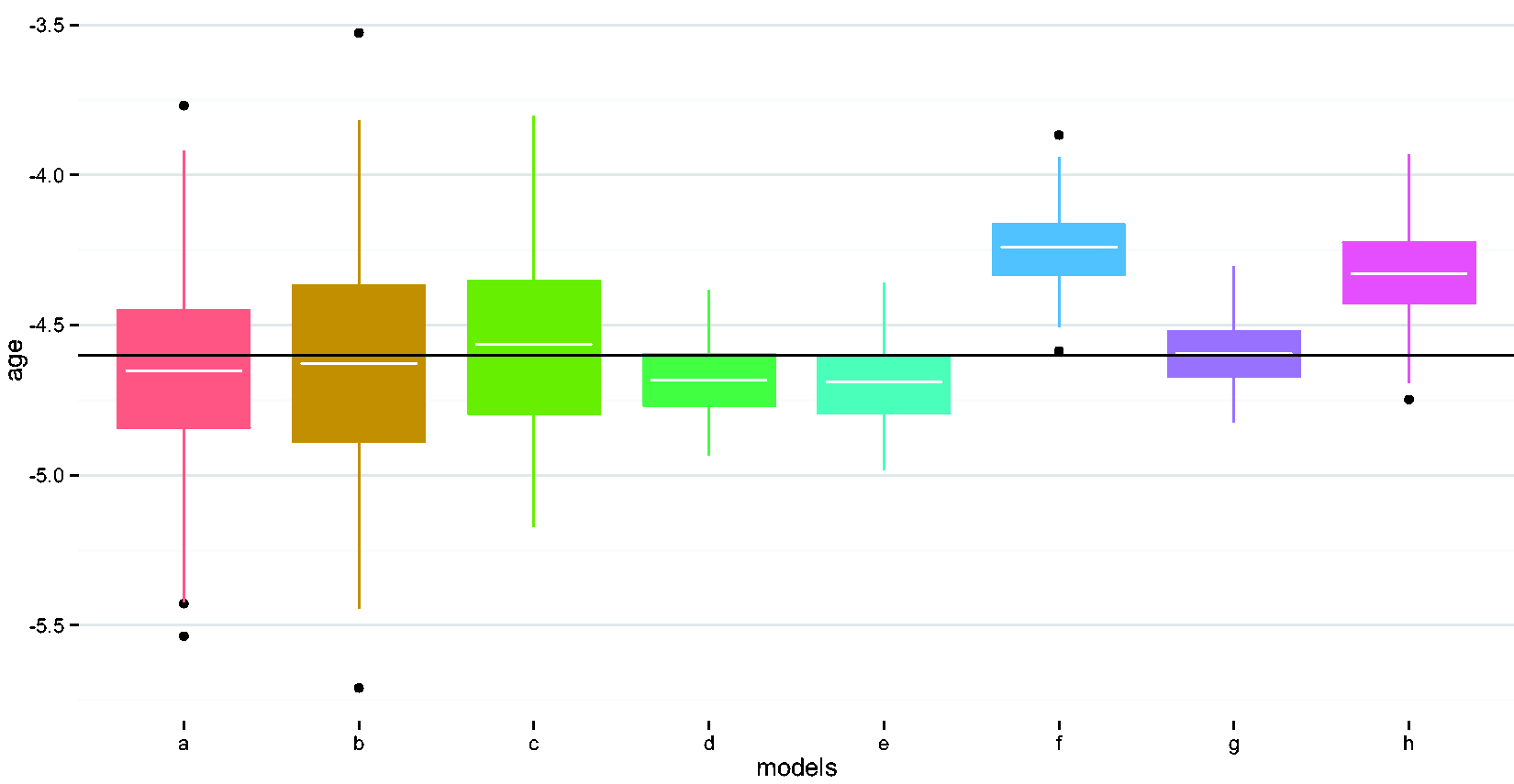
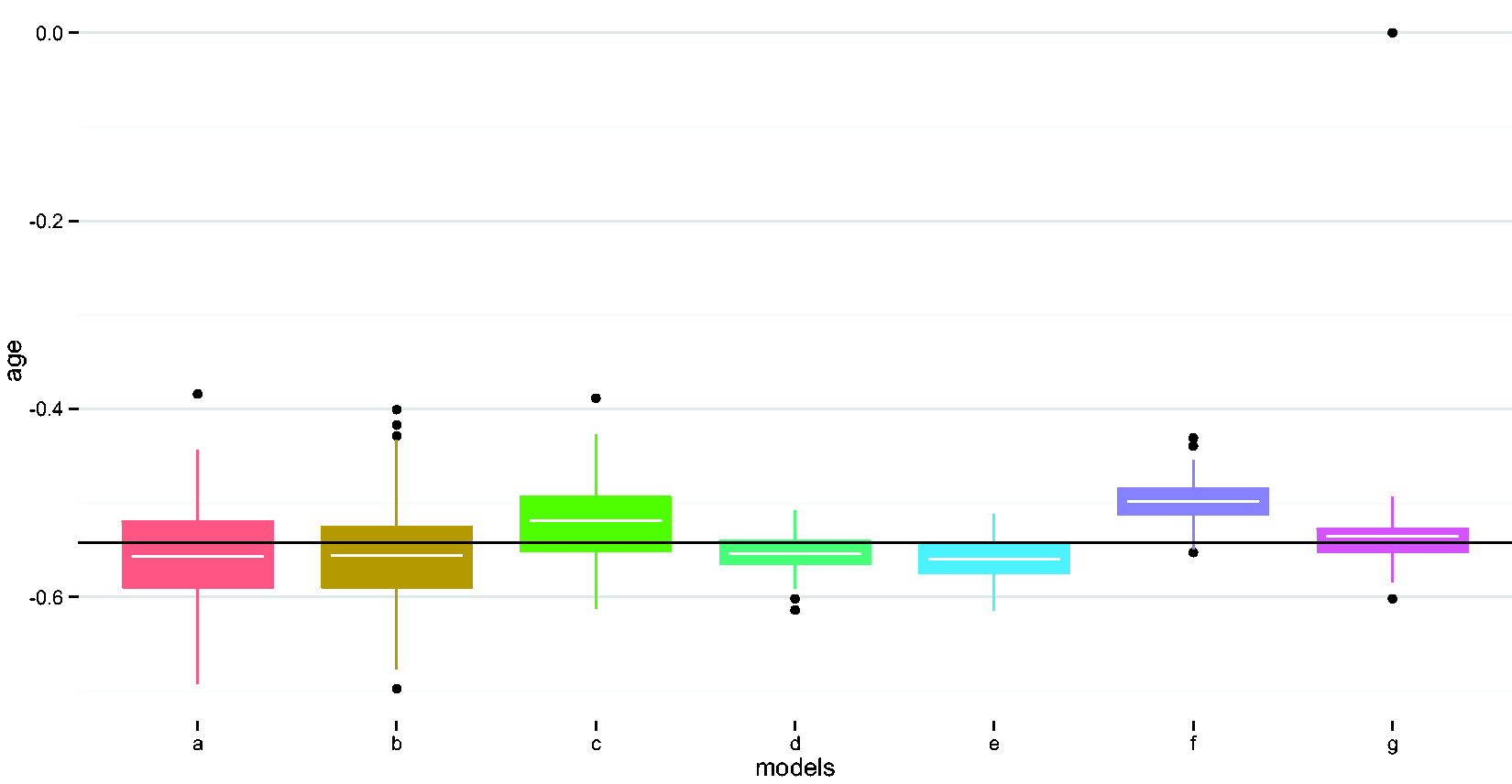
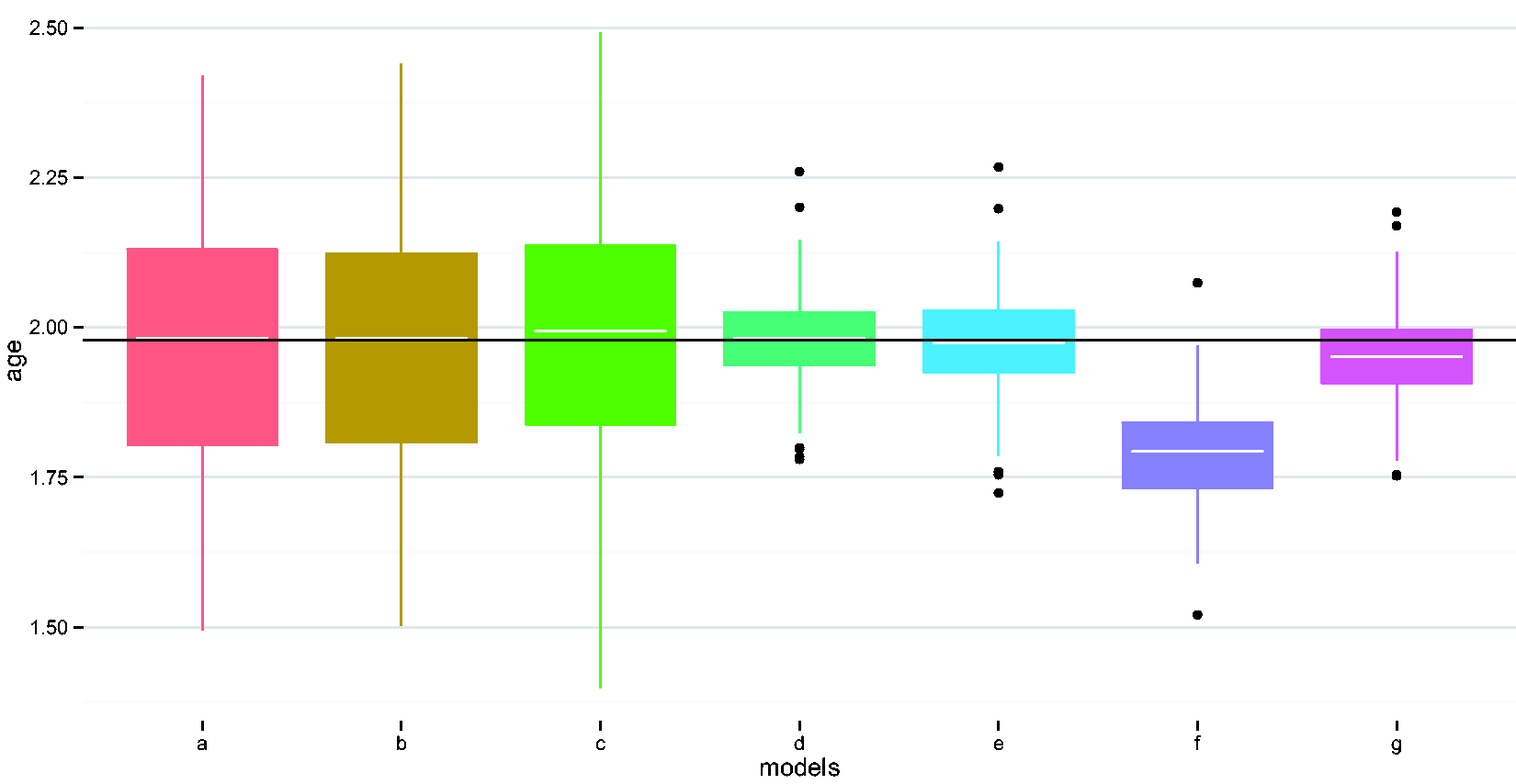
Compare performances of different methods in estimating the age coefficient. (a) Naïve model, (b) adjust for wear time, (c) EM imputation, (d) weighted regression i, (e) weighted regression ii, (f) imputed sum i, (g) imputed sum ii, and (h) K-NN. EM: expectation maximization; K-NN: K-nearest neighbor.

Figure 6.

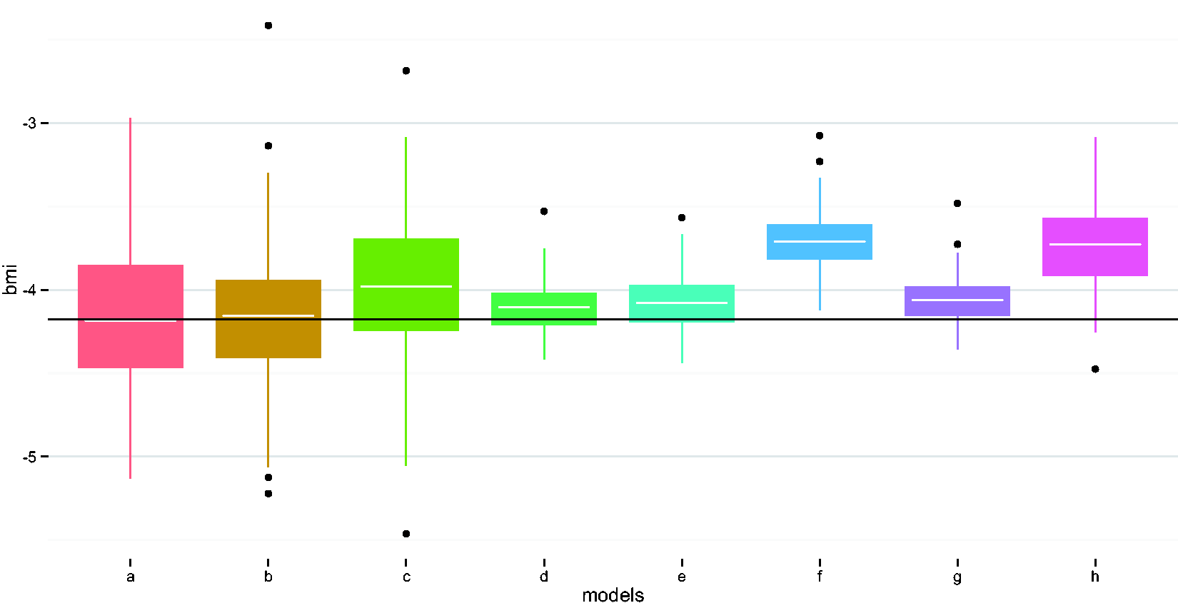
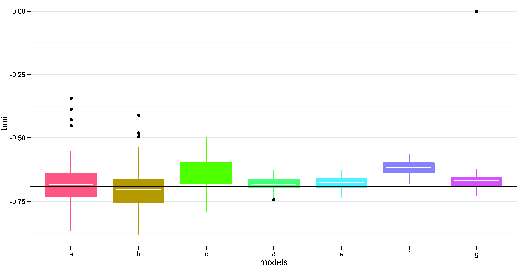
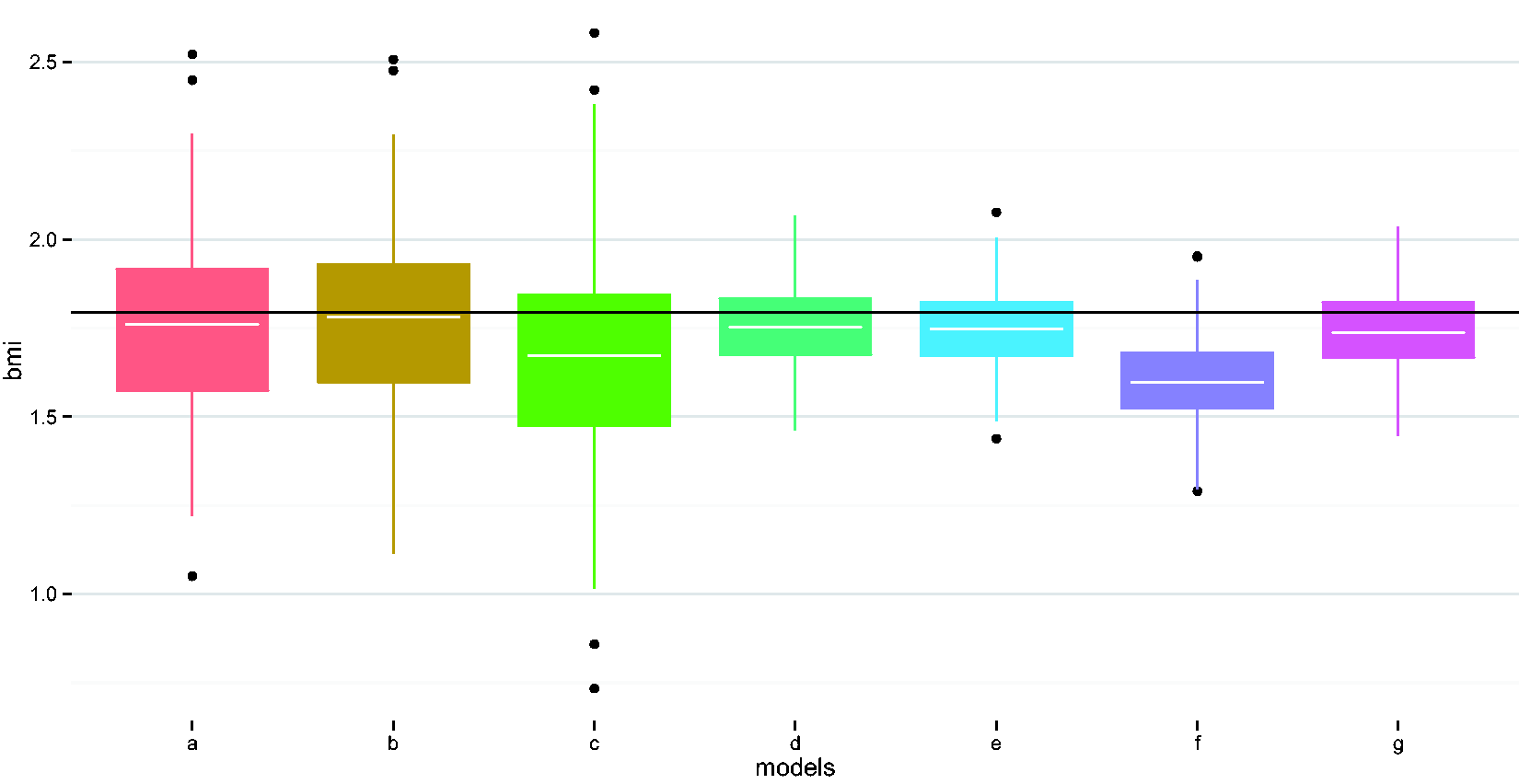
Compare performances of different methods in estimating the BMI coefficient. (a) Naïve model, (b) adjust for wear time, (c) EM imputation, (d) weighted regression i, (e) weighted regression ii, (f) imputed sum i, (g) imputed sum ii, and (h) K-NN. EM: expectation maximization; K-NN: K-nearest neighbor.

Figure 7.

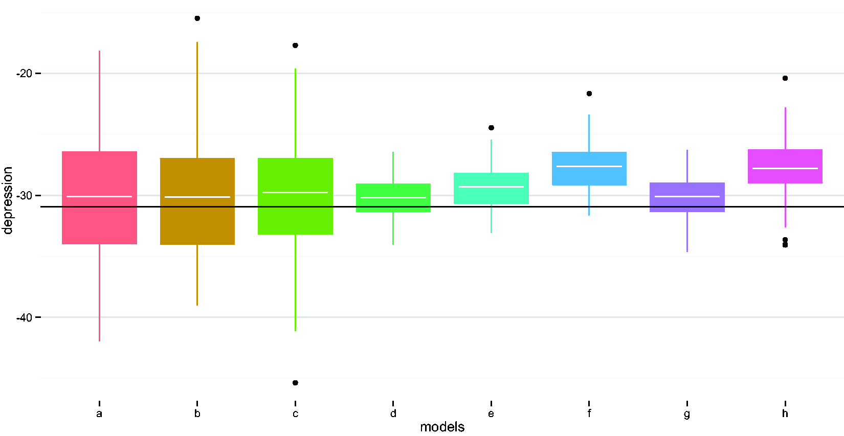
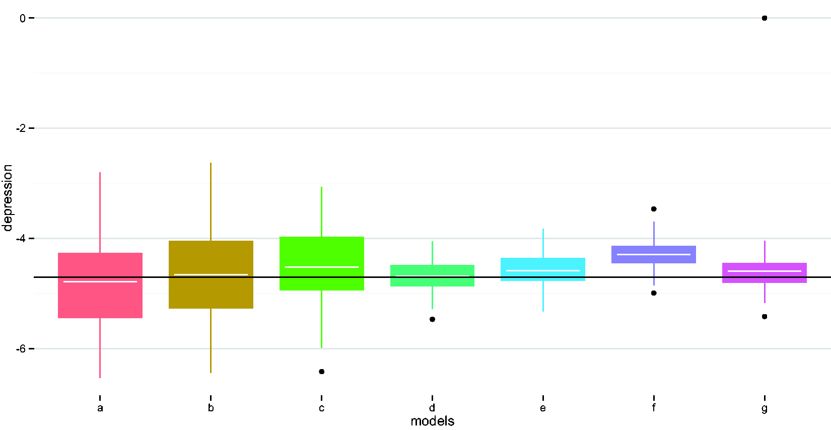
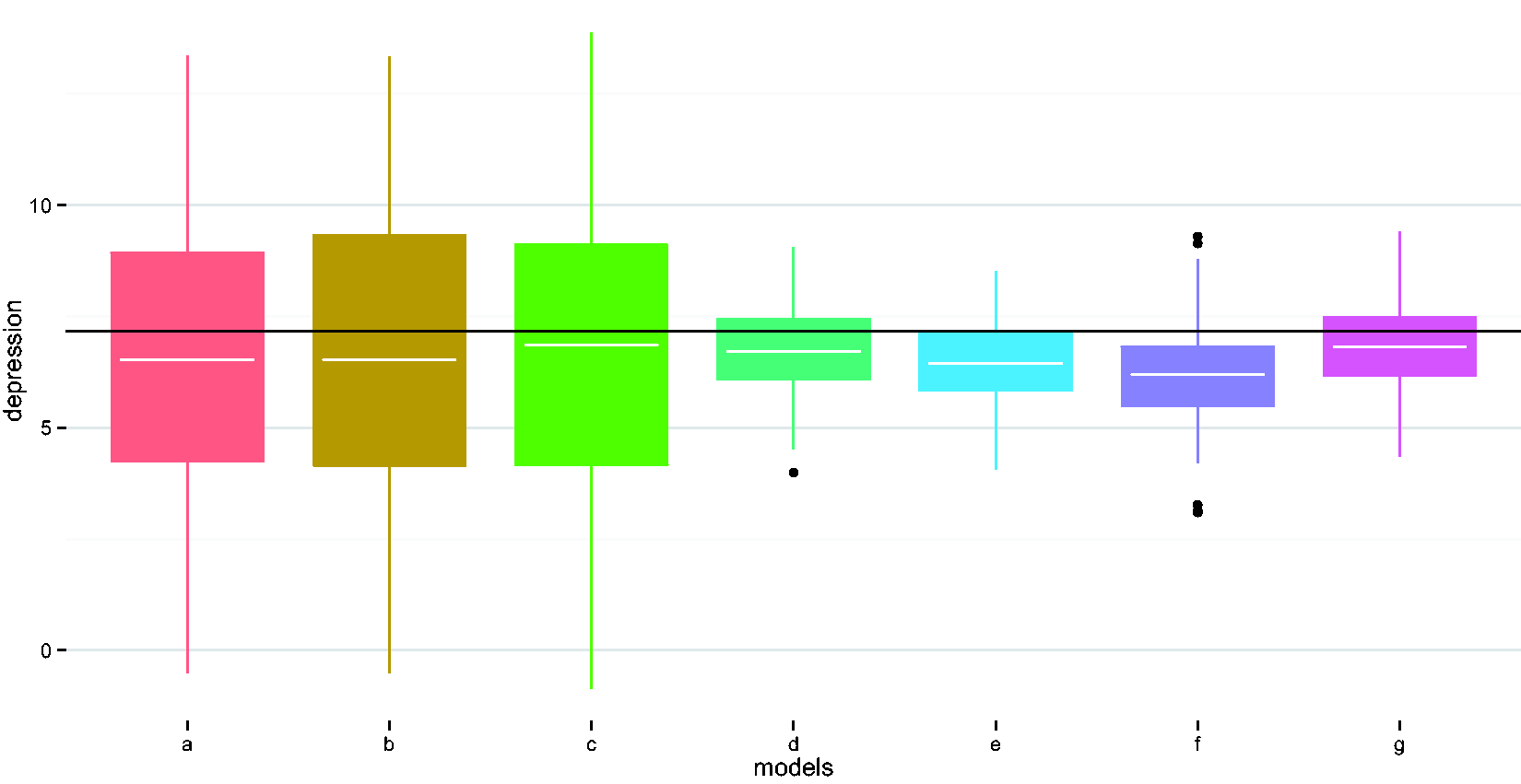
Compare performances of different methods in estimating the depression indicator coefficient. (a) Naïve model, (b) adjust for wear time, (c) EM imputation, (d) weighted regression i, (e) weighted regression ii, (f) imputed sum i, (g) imputed sum ii, and (h) K-NN. EM: expectation maximization; K-NN: K-nearest neighbor.

Figure 8.

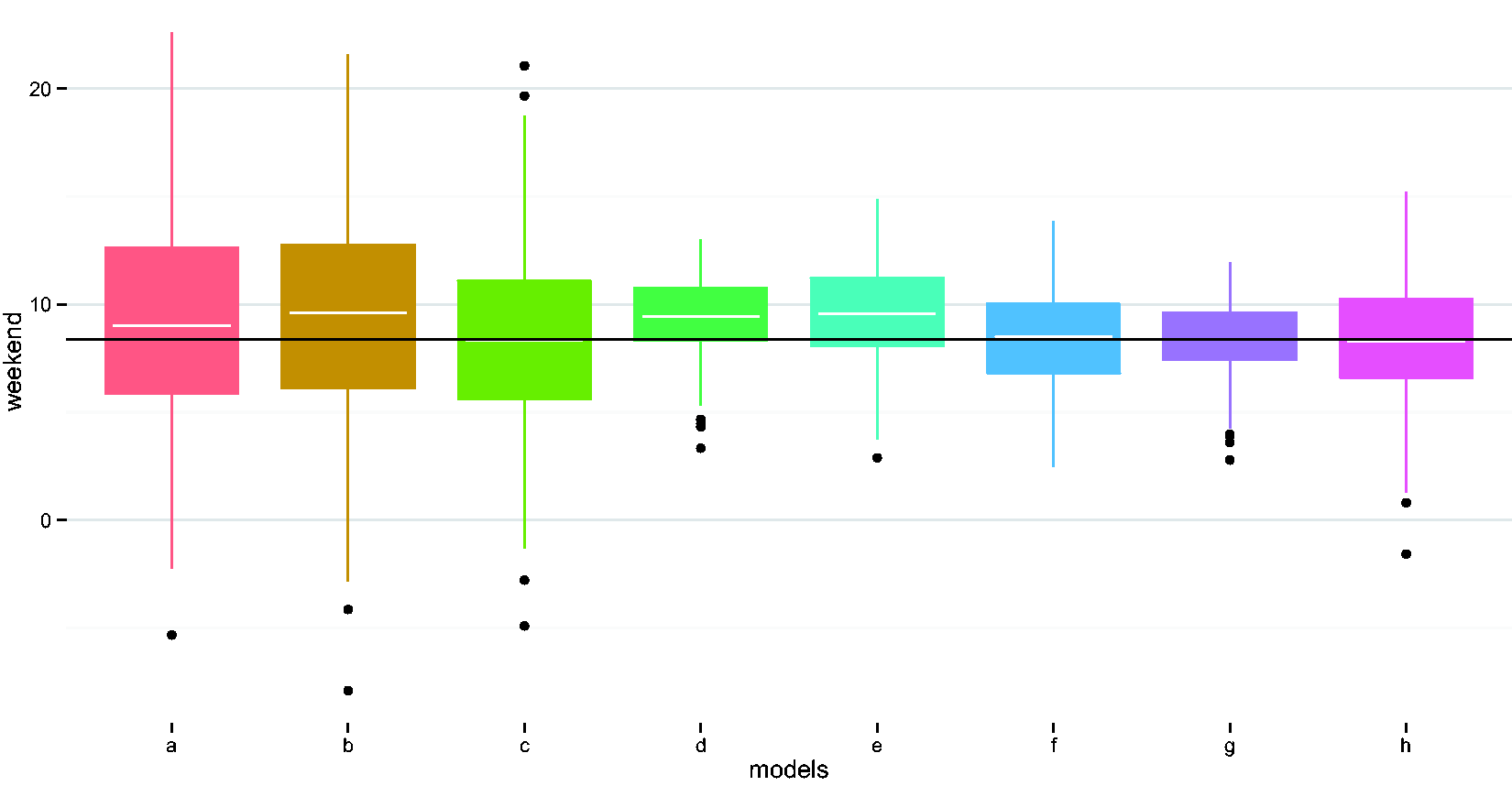
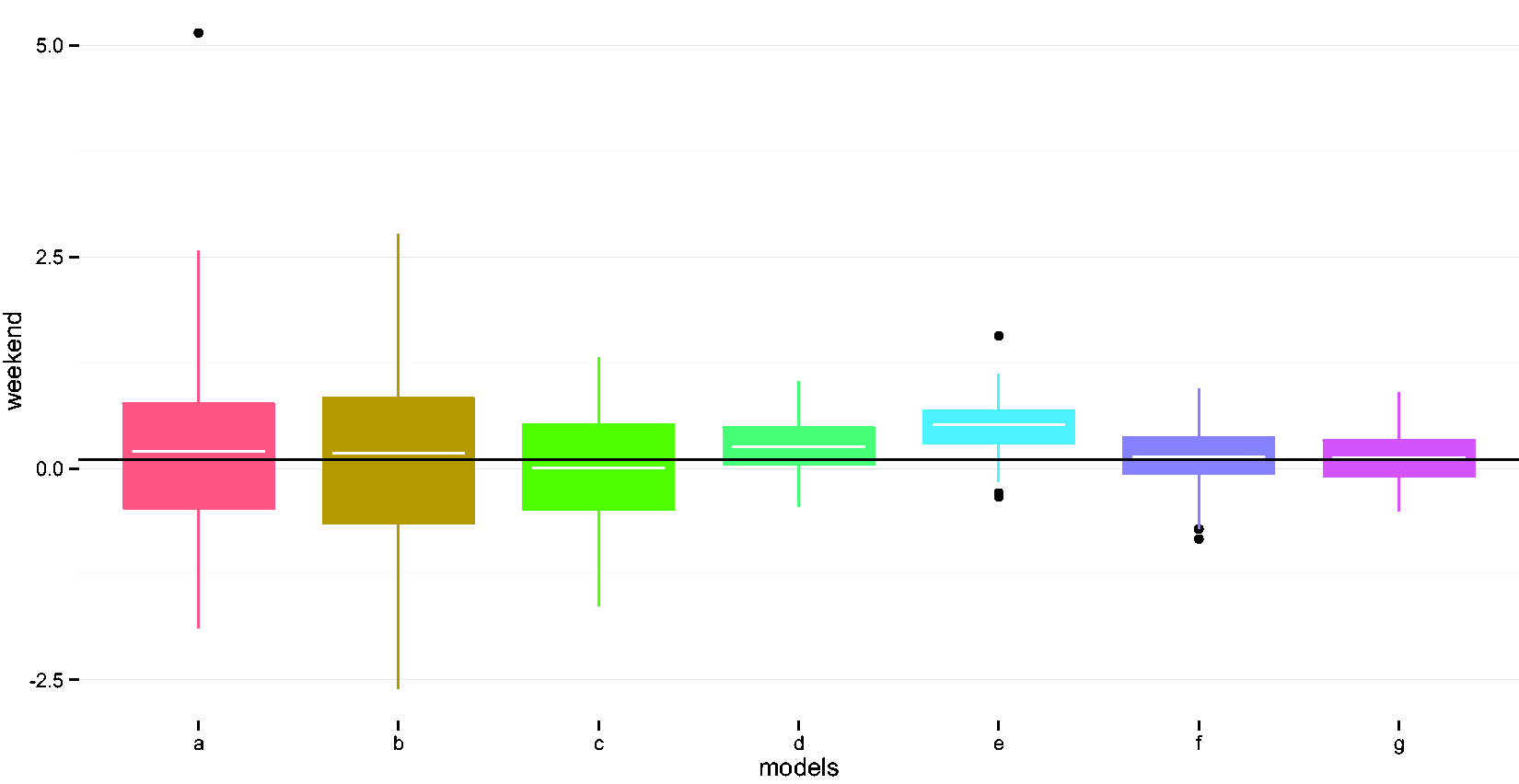
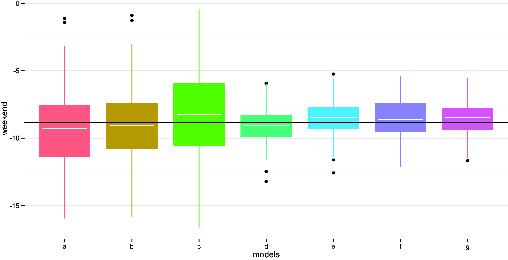
Compare performances of different methods in estimating the weekend indicator coefficient. (a) Naïve model, (b) adjust for wear time, (c) EM imputation, (d) weighted regression i, (e) weighted regression ii, (f) imputed sum i, (g) imputed sum ii, (h) K-NN. EM: expectation maximization; K-NN: K-nearest neighbor.

Results indicate that the naïve method, i.e. not accounting for missing data, and the conventional methods, i.e. (1) including wear time as a covariate in the model; (2) using an EM algorithm to impute average activities for the incomplete profiles,¹⁶ produced similar results. These three methods had the highest values for SDs for all covariates. The two conventional methods had higher values of relative efficiency than most methods proposed in the paper. Incorporating variance weights and/or subject-level imputation with random slope (method ii) compared to naïvely ignoring missing data, reduced mean-square error by over 75%. As expected, compared to the naïve and conventional methods, incorporating variance weights improved precision, with reductions in SDs > 50%, but did not reduce bias. The imputed sum methods also improved precision by > 50%, with varying impacts on bias. The K-NN method improved MSE for the binary variables, but did not perform as well as the weighted regressions or the imputed sum methods. All the proposed new methods improved coverage as compared to the naïve method.

Interestingly, the naïve and conventional methods exhibited lower bias compared to the other methods, especially for the continuous covariates, age and BMI. However, this lower bias was negligible in practical terms. For example, the average bias for BMI using the conventional method of adjusting for wear time as a covariate was 0.023 versus 0.467 for the imputed sum i. method, which had the highest average bias among all the methods (Table 1). Converting to regression slopes, this bias translates on average to 4.177 (true model), 4.2 (adjust for wear time model), and 3.71 (imputed sum i.) lower activity counts per minute for a 1 unit higher BMI, indicating minimal differences. Of note, the best performing methods also had minimal biases, with estimated average activity count decreases of 4.106 (variance weighting i.) and 4.06 (imputed sum ii.) per unit increase in BMI. In summary, our top overall (i.e. for MSE) performers were the weighted regression with weights proportional to reciprocal of the daily wear time percentage and the imputed daily sum method ii, which incorporated a random slope in the imputation model.

8 Other physical activity outcomes

Thus far, our analysis has focused on the total volume of activity accumulated throughout the day as the measure of physical activity. However, physical activity accumulation above or below an intensity threshold is also of interest in public health research. Hence it is important to investigate how our methods to account for missing data in accelerometry perform for other physical activity variables. In the following sections, we will examine two additional measures, namely daily minutes of moderate-vigorous physical activity (MVPA) and daily minutes of sedentary time, both of which have emerged as important factors for health.^1–4

8.1 Moderate-Vigorous Physical Activity (MVPA)

As in Section 3 our objective is to identify factors associated with MVPA in our original regression model (1). MVPA is measured as accelerometer counts above the threshold of 1951 counts. Variation in daily accelerometer wear time could lead to biased estimates of daily MVPA, making it difficult to compare MVPA across days and participants. Hence we created a standardized “MVPA” variable defined as the number of minutes of MVPA in a day if the wear time during the day were 720 min. Thus in practice, we would estimate MVPA as MVPA $= \frac{number of minutes of MVPA}{total wear time} \times 720$ . We repeated the regression analysis (Section 3) with this standardized MVPA as the dependent variable. As before, we fitted linear mixed models to the complete profiles, and used the estimated coefficients as the ground-truth to test the performance of our missing-data-correction methods. In the following, we will refer to this standardized MVPA variable, as simply MVPA, except when clarification is required.

Coefficient estimates for the associations between age, BMI, depression, and weekend indicator with MVPA in the complete profiles were $β_{1} = - 0.542$ (SE = 0.122), $β_{2} = - 0.692$ (SE = 0.170), $β_{3} = - 4.704$ (SE = 1.704), and $β_{4} = 0.101$ (SE = 0.738), respectively. Moreover, β₁, β₂, and β₃ were significant at a 1% significance level; β₄ was significant at 50% significance level.

We then applied our missing data correction methods to the pseudosimulated data generated in Section 5. The assumptions and the methods were similar to those described in Section 6. The only change was in Method 2, where the response variable for imputation was now number of minutes of MVPA instead of sum of activity. We also omitted the K-NN method since it performed poorly in our previous analysis and is computationally demanding.

Table 2 gives a numerical summary comparing performance of the different methods in terms of relative efficiency, bias, sim SD, and coverage. Figures 9 to 12 provide graphical comparisons of coefficient estimates across methods. Results were generally similar to the previous results. The naïve method (i.e. not accounting for missing data) yielded unstable estimates, albeit with minimal bias. Including wear time as a covariate in the model produced very similar results to the naïve method. Using an EM algorithm to impute MVPA for the incomplete profiles had smaller MSE than the naïve or conventional adjustment method, but was generally more biased. Imputation daily sum method i. with random intercepts (and fixed slope) had the highest bias for three of the predictors, but had lower MSE than the conventional methods. Subject-level imputation with random slope (method ii) compared to ignoring missing data, generally reduced mean-square error by > 30%, and improved precision and coverage. The weighted regressions performed the best with > 60% reductions in MSE and sim SD, and negligible bias compared to the naïve method; the top performer was weighted regression with weights proportional to reciprocal of the daily wear time percentage.

Table 2.

Comparison of methods for moderate-vigorous physical activity.

		Relative efficiency	Bias	Sim SD	Coverage
Naïve model	Age	1.000	−0.014	0.054	1.00
	BMI	1.000	0.009	0.088	0.96
	Depression	1.000	−0.080	0.844	0.47
	Weekend	1.000	0.100	1.095	0.26
Adjust for wear time	Age	1.073	−0.014	0.057	0.98
	BMI	0.825	−0.013	0.079	0.96
	Depression	0.930	0.042	0.817	0.40
	Weekend	0.955	0.077	1.072	0.29
EM imputation	Age	0.806	0.023	0.045	1.00
	BMI	0.785	0.054	0.057	1.00
	Depression	0.676	0.185	0.672	0.94
	Weekend	0.417	−0.098	0.703	0.27
Weighted regression i	Age	0.161	−0.012	0.019	1.00
	BMI	0.085	0.008	0.024	1.00
	Depression	0.089	0.015	0.253	0.87
	Weekend	0.104	0.153	0.320	0.58
Weighted regression ii	Age	0.232	−0.017	0.021	1.00
	BMI	0.120	0.016	0.026	1.00
	Depression	0.136	0.122	0.288	0.70
	Weekend	0.232	0.412	0.331	0.48
Imputed sum i	Age	0.760	0.044	0.021	1.00
	BMI	0.774	0.074	0.025	1.00
	Depression	0.341	0.416	0.269	0.84
	Weekend	0.104	0.037	0.352	0.52
Imputed sum ii	Age	1.049	0.007	0.057	0.99
	BMI	0.721	0.024	0.071	0.99
	Depression	0.398	0.115	0.523	0.87
	Weekend	0.075	0.030	0.299	0.52

BMI: Body Mass Index; EM: expectation maximization; sim SD: simulation standard deviation.

Relative efficiency: ratio of mean-squared error between the current method and the naïve model; Coverage: percentage of times null is rejected under the corresponding true model significance level, and the coefficient estimates have the correct sign; “Naïve” model disregarded missing data. “Adjust for wear time” model included wear time as a covariate. “EM imputation” model used EM algorithm to impute MVPA for the incomplete profiles.

Figure 9.

Compare performances of different methods in estimating the age coefficient. (a) Naïve model, (b) adjust for wear time, (c) EM imputation, (d) weighted regression i, (e) weighted regression ii, (f) imputed sum i, and (g) imputed sum ii. EM: expectation maximization.

Figure 10.

Compare performances of different methods in estimating the BMI coefficient. (a) Naïve model, (b) adjust for wear time, (c) EM imputation, (d) weighted regression i, (e) weighted regression ii, (f) imputed sum i, and (g) imputed sum ii. EM: expectation maximization.

Figure 11.

Compare performances of different methods in estimating the depression indicator coefficient. (a) Naïve model, (b) adjust for wear time, (c) EM imputation, (d) weighted regression i, (e) weighted regression ii, (f) imputed sum i, and (g) imputed sum ii. EM: expectation maximization.

Figure 12.

Compare performances of different methods in estimating the weekend indicator coefficient. (a) Naïve model, (b) adjust for wear time, (c) EM imputation, (d) weighted regression i, (e) weighted regression ii, (f) imputed sum i, and (g) imputed sum ii. EM: expectation maximization.

8.2 Sedentary time

In this section we examined how our correction methods performed if sedentary time was the outcome. Sedentary time is measured as accelerometer counts below the threshold of 100 counts. Again, our estimate of daily sedentary time took into account the total wear time during that day. Thus, “standardized sedentary time” was defined as the number of minutes of sedentary time in a day if the wear time during the day were 720 min, i.e. Sedentary Time $= \frac{number of minutes of sedentary time}{total wear time} \times 720$ . We repeated the regression analysis (Section 3) with this standardized sedentary time as the dependent variable. As before, we fitted linear mixed models to the complete profiles and used the estimated coefficients as the ground-truth to test the performance of our missing-data-correction methods. In the following, we will refer to this standardized sedentary time variable, as simply sedentary time, except when clarification is required.

Coefficient estimates for the associations between age, BMI, depression, and weekend indicator with sedentary time in the complete profiles were $β_{1} = 1.979$ (SE = 0.550), $β_{2} = 1.793$ (SE = 0.767), $β_{3} = 7.169$ (SE = 7.704), and $β_{4} = - 8.852$ (SE = 2.953), respectively. Moreover, β₁ and β₄ were significant at 1% significance level; β₂ was significant at 5% significance level; β₃ was significant at the 50% significance level.

We then applied our missing data correction methods to the pseudosimulated data generated in Section 5. The assumptions and the methods were similar to those described in Section 6. The only change was in Method 2, where the response variable for imputation was now number of minutes of sedentary time instead of sum of activity. We again omitted the K-NN method since it performed poorly in our previous analysis and is computationally demanding.

Table 3 gives a numerical summary comparing performance of the different methods in terms of relative efficiency, bias, sim SD, and coverage. Figures 13 to 16 provide graphical comparisons of coefficient estimates across methods. The naïve method, i.e. not accounting for missing data, and the conventional methods, i.e. (1) including wear time as a covariate in the model and (2) using EM algorithm to impute sedentary time for incomplete profiles, produced similar, if not worse, results. These methods exhibited the smallest bias, especially for the continuous covariates, but large SDs for all the covariates, resulting in large mean-squared errors. Imputed daily sum method i. with random intercepts generally had the highest bias. Each of the proposed new methods, i.e. incorporating variance weights or subject-level imputation, improved precision (sim SD) by > 40%, and improved coverage by > 25%. Our top overall performers in terms of mean-squared error were the weighted regression with weights proportional to reciprocal of the daily wear time percentage and the imputed daily sum method ii, which incorporated a random slope in the imputation model; these methods, compared to the conventional methods, reduced MSE by >75% for all the covariates.

Table 3.

Comparison of methods for sedentary time.

		Relative efficiency	Bias	Sim SD	Coverage
Naïve model	Age	1.000	0.003	0.210	1.00
	BMI	1.000	−0.032	0.259	0.73
	Depression	1.000	−0.646	3.102	0.61
	Weekend	1.000	−0.418	2.903	0.29
Adjust for wear time	Age	0.988	0.003	0.209	1.00
	BMI	0.996	−0.011	0.260	0.78
	Depression	1.008	−0.633	3.118	0.61
	Weekend	0.975	−0.227	2.886	0.26
EM imputation	Age	1.108	0.015	0.220	1.00
	BMI	1.776	−0.120	0.327	0.89
	Depression	1.189	−0.308	3.442	0.73
	Weekend	1.287	0.592	3.274	0.39
Weighted regression i	Age	0.163	0.004	0.084	1.00
	BMI	0.202	−0.041	0.110	0.98
	Depression	0.128	−0.455	1.036	0.91
	Weekend	0.194	−0.231	1.272	0.81
Weighted regression ii	Age	0.203	−0.004	0.094	1.00
	BMI	0.212	−0.046	0.111	0.98
	Depression	0.157	−0.723	1.026	0.85
	Weekend	0.224	0.405	1.326	0.51
Imputed sum i	Age	0.938	−0.185	0.083	1.00
	BMI	0.841	−0.195	0.139	0.92
	Depression	0.243	−0.977	1.218	0.88
	Weekend	0.260	0.229	1.479	0.72
Imputed sum ii	Age	0.174	−0.027	0.083	1.00
	BMI	0.231	−0.056	0.112	0.97
	Depression	0.120	−0.357	1.039	0.93
	Weekend	0.169	0.378	1.143	0.84

BMI: Body Mass Index; EM: expectation maximization; sim SD: simulation standard deviation.

Figure 13.

Compare performances of different methods in estimating the age coefficient. (a) Naïve model, (b) adjust for wear time, (c) EM imputation, (d) weighted regression i, (e) weighted regression ii, (f) imputed sum i, and (g) imputed sum ii. EM: expectation maximization.

Figure 14.

Compare performances of different methods in estimating the BMI coefficient. (a) Naïve model, (b) adjust for wear time, (c) EM imputation, (d) weighted regression i, (e) weighted regression ii, (f) imputed sum i, and (g) imputed sum ii. EM: expectation maximization.

Figure 15.

Compare performances of different methods in estimating the depression indicator coefficient. (a) Naïve model, (b) adjust for wear time, (c) EM imputation, (d) weighted regression i, (e) weighted regression ii, (f) imputed sum i, and (g) imputed sum ii. EM: expectation maximization.

Figure 16.

Compare performances of different methods in estimating the weekend indicator coefficient. (a) Naïve model, (b) adjust for wear time, (c) EM imputation, (d) weighted regression i, (e) weighted regression ii, (f) imputed sum i, and (g) imputed sum ii. EM: expectation maximization.

9 Theoretical underpinning: A Poisson framework

The variance weighting method with weights inversely proportional to daily wear time percentage generally had the least error across all our analyses. We can justify this superior performance under a plausible Poisson generating mechanism for the accelerometer data. In particular, suppose that activity count at each minute follows a Poisson distribution with intensity parameter λ. We further assume that the proportion of daily wear time for subject i converges to a constant, denoted as $θ_{i} = θ$ . Now suppose that on a given day, we observe m_i = m minutes of activity for subject i (note: to reduce complexity of notation, we suppress the index i when referring to θ and m). We naïvely use the mean of these m Poisson activity readings to estimate the average activity for this day for subject i. Theoretically, under an iid assumption, this estimator has mean λ and variance $λ / m$ , which by our assumption will converge to $λ / (θ \times T)$ , where T denotes the ideal total number of minutes of device wear time in a day. Therefore, it is reasonable to set the variance of our regression model to be proportional to $1 / θ$ . Although this is a simplified model, we believe that using this Poisson framework provides a useful theoretical heuristic to explain the superior performance of the variance-weighted model.

10 Conclusions

Accurate measurement of physical activity is a critical factor for designing and implementing interventions aimed at modifying this important behavior. Accelerometers provide rich and objective data on individual-level physical activity patterns throughout the day, and hence have emerged as an important tool in physical activity research. Despite their many advantages, analysis of accelerometer data presents many challenges.¹⁵

In this paper, we focused on one specific challenge, namely missing data due to nonwear. Using a large cohort, we characterized patterns of accelerometer nonwear during the day, which is a critical first step to developing methods to correct for missing data. We observed that missing data patterns tended to occur at the beginning and end of the day. This observation is important for simulating realistic missing data patterns, i.e. randomly distributed nonwear throughout the day is atypical, and assuming a completely-at-random missingness pattern would not mimic what occurs in practice. Next, we used a pseudosimulation approach to develop and compare three new statistical approaches to correct for missing accelerometer data in a regression model setting with physical activity is the dependent variable of interest, such as in an intervention trial. For the sake of comparison, we also implemented two existing methods commonly used to account for device nonwear: including wear time as a covariate, and an EM-type imputation algorithm.¹⁶

Our results indicated that ignoring missing data had a major impact on precision (i.e. high standard errors of regression parameters). The conventional methods of including wear time as a covariate or an EM-type imputation did not improve precision. Among the proposed methods, (a) variance weighting by the inverse of daily wear time proportions and (b) imputing activity using subject-specific intercepts and slopes, improved precision the most, albeit with a small increase in bias for some covariates. However, the gain in precision far outweighed the increased bias, which was negligible in practical terms. Improving precision of regression estimates has major implications for study design: large variability requires larger sample sizes to ensure adequate power. Equivalently, ignoring nonwear or controlling for wear time may result in failure to reject a null hypothesis. Of note, our variance weighting method has a theoretical basis under a Poisson framework, while the imputation method exploits the hierarchical nature of the data, namely day-level information nested within subjects.

A few limitations need to be noted. First, our cohort comprised of postmenopausal breast cancer survivors, which could limit generalizability. It is possible that a different sample may exhibit a different missing data pattern. However, other studies^16,32 have noted concentrated missing data patterns, similar to what we observed. Second, our sample used a wake-time protocol for hip-worn accelerometers. Wrist-worn and small hip-worn accelerometers, which can be worn for 24 h, are gaining in popularity and may have fewer problems with device nonwear, since participants are more likely to wear the devices for longer periods. But 24 h protocols do not result in 24 h of wear, and variation in wear time may, in fact, increase with longer wear periods, making it even more important to consider statistical adjustments for nonwear when analyzing these data. Furthermore, intensity cutpoints for wrist accelerometers have not been standardized, and many different algorithms have been proposed for classifying activity level.^33–35 Besides, hip-worn devices have been used to measure physical activity in several large existing cohorts comprising over 50,000 participants,³⁶ including subsets of the NHANES database,³⁷ and the OPACH substudy of the Women’s Health Initiative.³⁸ These unique and well-characterized databases include information on a variety of cardiovascular, cancer, psychosocial, and other outcomes, resulting in unique data sources for examining physical activity–disease associations. Hence statistical methods for missing data for these hip devices are still highly relevant in public health research. Importantly, our proposed statistical approaches are generalizable, and we do not expect the choice of cohort or device to have a major impact on how these new statistical methods will perform. Third, our analysis focused on physical activity as a dependent variable and examined its correlates. We did not investigate if our methods would also correct biases in models where physical activity is an independent variable. Although the mixed-effects and K-NN imputation methods are easily applicable to the latter case, such analyses are fundamentally different from our setting, and we leave their investigation to a future project. Finally, we note that statistical methods using functional data analysis^39,40 to model minute-level accelerometer data are being increasingly proposed. These methods implement minute-level interpolation or imputation via likelihood or Bayesian methods to account for nonwear. While these minute-level methods hold promise, they are complex and computationally challenging. Of note, and perhaps surprisingly, in our simulations, the EM algorithm, a standard method for missing data imputation, and K-NN, which considers time of day in the imputation algorithm, both were outperformed by the simpler variance weighting and imputed sums methods. A possible reason for this is that when the unit of analysis is day-level activity, these more complex methods may actually introduce more variance. Thus, the methods we propose are easy to implement using standard software and hence will be accessible to the applied statistician or epidemiologist.

In summary, we introduce two new methods to account for nonwear in accelerometer-based physical activity research. We considered three measures of physical activity: total volume summarized as daily accelerometer counts per minute, daily minutes of MVPA, and daily minutes of sedentary time. Our results were consistent across the three activity measures, and indicated that implementing variance-weighting or imputation using subject-specific parameters could vastly reduce variability in parameter estimates, thus improving study power. There is a bias-variance trade-off whereby the proposed methods could lead to increased bias, but as noted these biases were negligible and of little practical importance. We anticipate that these easy-to-implement correction methods will be useful in physical activity research.

Footnotes

Acknowledgements

The content of this article is solely the responsibility of the authors and does not necessarily represent the official views of the National Institutes of Health.

Declaration of conflicting interests

The author(s) declared no potential conflicts of interest with respect to the research, authorship, and/or publication of this article.

Funding

The author(s) disclosed receipt of the following financial support for the research, authorship, and/or publication of this article: SYX was supported by a UCSD Chancellor’s Frontiers of Innovation Scholars Program Fellowship; JK, SG, RP, LN were partially supported by funding from the National Cancer Institute (U54 CA155435-01).

References

Bijnen

Caspersen

Mosterd

. Physical inactivity as a risk factor for coronary heart disease: a WHO and International Society and Federation of Cardiology position statement. Bull World Health Organ 1994; 72: 1–4.

Sullivan

Morrato

Ghushchyan

et al.

Obesity, inactivity, and the prevalence of diabetes and diabetes-related cardiovascular comorbidities in the U.S., 2000–2002. Diabetes Care 2005; 28: 1599–1603.

Blair

. Physical inactivity: the biggest public health problem of the 21st century. Br J Sports Med 2009; 43: 1–2.

Wilmot

Edwardson

Achana

et al.

Sedentary time in adults and the association with diabetes, cardiovascular disease and death: systematic review and meta-analysis. Diabetologia 2012; 55: 2895–2905.

Sallis

Saelens

. Assessment of physical activity by self-report: status, limitations, and future directions. Res Q Exerc Sport 2000; 71: S1–14.

Prince

Adamo

Hamel

et al.

A comparison of direct versus self-report measures for assessing physical activity in adults: a systematic review. Int J Behav Nutr Phys Act 2008; 5: 56–56.

Ward

Evenson

Vaughn

et al.

Accelerometer use in physical activity: best practices and research recommendations. Med Sci Sports Exerc 2005; 37: S582–S588.

Kang

Bassett

Barreira

et al.

How many days are enough? A study of 365 days of pedometer monitoring. Res Q Exerc Sport 2009; 80: 445–453.

Herrmann

Barreira

Kang

et al.

How many hours are enough? Accelerometer wear time may provide bias in daily activity estimates. J Phys Act Health 2013; 10: 742–749.

10.

Herrmann

Barreira

Kang

et al.

Impact of accelerometer wear time on physical activity data: a NHANES semisimulation data approach. Br J Sports Med 2014; 48: 278–282.

11.

Trost

McIver

Pate

. Conducting accelerometer-based activity assessments in field-based research. Med Sci Sports Exerc 2005; 37: S531–S543.

12.

Merchant

Buelna

Castañeda

et al.

Accelerometer-measured sedentary time among Hispanic adults: results from the Hispanic Community Health Study/Study of Latinos (HCHS/SOL). Prevent Med Rep 2015; 2: 845–853.

13.

Colley

Connor Gorber

Tremblay

. Quality control and data reduction procedures for accelerometry-derived measures of physical activity. Health Rep 2010; 21: 63–69.

14.

Young

Jerome

Chen

et al.

Patterns of physical activity among overweight and obese adults. Prev Chronic Dis 2009; 6: A90–A90.

15.

Staudenmayer

Zhu

Catellier

. Statistical considerations in the analysis of accelerometry-based activity monitor data. Med Sci Sports Exerc 2012; 44: S61–S67.

16.

Catellier

Hannan

Murray

et al.

Imputation of missing data when measuring physical activity by accelerometry. Med Sci Sports Exerc 2005; 37: S555–S562.

17.

Wilson

Van Horn

Siceloff

et al.

The Results of the Positive Action for Today’s Health (PATH) trial for increasing walking and physical activity in underserved African-American communities. Ann Behav Med 2015; 49: 398–410.

18.

Kang

Rowe

Barreira

et al.

Individual information-centered approach for handling physical activity missing data. Res Q Exerc Sport 2009; 80: 131–137.

19.

Katapally

Muhajarine

. Towards uniform accelerometry analysis: a standardization methodology to minimize measurement bias due to systematic accelerometer wear-time variation. J Sports Sci Med 2014; 13: 379–386.

20.

Shiroma

Freedson

Trost

et al.

Patterns of accelerometer-assessed sedentary behavior in older women. JAMA 2013; 310: 2562–2563.

21.

van Landingham

Willis

Vitale

et al.

Visual field loss and accelerometer-measured physical activity in the United States. Ophthalmology 2012; 119: 2486–2492.

22.

Colley

Garriguet

Janssen

et al.

Physical activity of Canadian adults: accelerometer results from the 2007 to 2009 Canadian Health Measures Survey. Health Rep 2011; 22: 7–14.

23.

Troiano

Berrigan

Dodd

et al.

Physical activity in the United States measured by accelerometer. Med Sci Sports Exerc 2008; 40: 181–188.

24.

Patterson

Marinac

Natarajan

et al.

Recruitment strategies, design, and participant characteristics in a trial of weight-loss and metformin in breast cancer survivors. Contemp Clin Trials 2015; S1551–7144: 30140–30143.

25.

Bassett

. Device-based monitoring in physical activity and public health research. Physiol Meas 2012; 33: 1769–1783.

26.

Choi

Liu

Matthews

et al.

Validation of accelerometer wear and non-wear time classification algorithm. Med Sci Sports Exerc 2011; 43: 357–364.

27.

Diggle Diggle

Heagerty

Liang

et al.

Analysis of longitudinal data, Oxford: Oxford Univ. Press, 2013.

28.

Pinheiro J, Bates D, DebRoy S, et al. R Core Team, nlme: linear and nonlinear mixed effects models. R package version 3.1-122, 2015.

29.

Hastie

Tibshirani

Friedman

. The elements of statistical learning, Berlin Heidelberg: Springer, 2001.

30.

Schafer JL. Analysis of incomplete multivariate data. Monographs on statistics and applied probability, vol. 72. Chapman and Hall/CRC, Boca Raton, FL, 2000.

31.

Honaker

King

Blackwell

. Amelia II: a program for missing data. J Statist Softw 2011; 45: 1–47.

32.

Sani

Refinetti

Jean-Louis

et al.

Daily activity patterns of 2316 men and women from five countries differing in socioeconomic development. Chronobiol Int 2015; 32: 650–656.

33.

Ellis

Kerr

Godbole

et al.

Hip and wrist accelerometer algorithms for free-living behavior classification. Med Sci Sports Exerc 2016; 48(5): 933–40.

34.

Hickey

Newham

Slawinska

et al.

Estimating cut points: a simple method for new wearables. Maturitas 2016; 83: 78–82.

35.

Swartz

Strath

Bassett

Jr et al.

Estimation of energy expenditure using CSA accelerometers at hip and wrist sites. Med Sci Sports Exerc 2000; 32: S450–S456.

36.

Lee

Shiroma

. Using accelerometers to measure physical activity in large-scale epidemiologic studies: issues and challenges. Br J Sports Med 2014; 48: 197201–197201.

37.

NHANES, http://www.cdc.gov/nchs/nhanes.htm (accessed 20 January 2016).

38.

OPACH Study, https://www.whi.org/studies/SitePages/Home.aspx (accessed 20 June 2016).

39.

Morris

Arroyo

Coull

et al.

Using wavelet-based functional mixed models to characterize population heterogeneity in accelerometer profiles: a case study. J Am Stat Assoc 2006; 101: 1352–1364.

40.

Xiao

Huang

Schrack

et al.

Quantifying the lifetime circadian rhythm of physical activity: a covariate-dependent functional approach. Biostatistics 2015; 16: 352–367.