Multiscale measurement error models for aggregated small area health data

Abstract

Spatial data are often aggregated from a finer (smaller) to a coarser (larger) geographical level. The process of data aggregation induces a scaling effect which smoothes the variation in the data. To address the scaling problem, multiscale models that link the convolution models at different scale levels via the shared random effect have been proposed. One of the main goals in aggregated health data is to investigate the relationship between predictors and an outcome at different geographical levels. In this paper, we extend multiscale models to examine whether a predictor effect at a finer level hold true at a coarser level. To adjust for predictor uncertainty due to aggregation, we applied measurement error models in the framework of multiscale approach. To assess the benefit of using multiscale measurement error models, we compare the performance of multiscale models with and without measurement error in both real and simulated data. We found that ignoring the measurement error in multiscale models underestimates the regression coefficient, while it overestimates the variance of the spatially structured random effect. On the other hand, accounting for the measurement error in multiscale models provides a better model fit and unbiased parameter estimates.

Keywords

Measurement error multiscale models scaling effect shared random effects convolution models

1 Introduction

It is of interest to model the relationship between spatially referenced health outcomes and predictors by taking into account the spatial uncertainty in the data. Spatial data are often observed in the form of aggregated counts at census tract, county, and state levels. These aggregations essentially smooth the data, that is to say that the variability in the data will be reduced and hence there will be loss of information. Using appropriate spatial statistical methods can help to alleviate the loss of information. Much work has been done to handle the variability in the outcome using spatially structured and unstructured random effects.¹ In addition, multiscale modeling has been used to model the aggregation of outcomes from one level to another level.² However, less emphasis has been given to modeling the uncertainty in outcomes when aggregation of predictors from one level (e.g., county) to another level (e.g., state) is considered. Since we cannot directly measure the predictor (e.g., income) at coarser levels, it is often approximated by aggregating the observed values of the predictor obtained from the individuals at the finest level. Hence, using the aggregated predictor as a proxy (surrogate) measure for the true unobserved predictor might induce measurement error (ME), i.e., predictor uncertainty due to aggregation.

Researchers usually model classical ME as follows. The true covariate is measured with additive error, i.e., W = X + U, where W is the error-prone covariate, X is the true unobserved covariate, and U is the ME structure.³ Since we cannot observe the true covariate X, we cannot fit directly the regression of Y on X. Hence, the aim of the classical ME modeling is to obtain unbiased estimates of parameters of the regression of Y on X indirectly by fitting Y on W after adjusting for ME.³ If we regress Y directly on W without accounting for the ME, it leads to biased estimates and loss of power for detecting relationships between variables. There are different methods that are applicable for ME analysis: regression calibration, simulation extrapolation (SIMEX), using instrumental variables (IVs), etc. In regression calibration, the main idea is to replace X by the regression of X on W and then doing a standard regression analysis. This is a simple, effective, and widely used method.⁴ Although regression calibration is often useful for generalized linear models, it can be rather poor for highly non-linear models.³

Alternatively, a computationally intensive and simulation-based method, known as SIMEX, has been considered to adjust for ME.⁵ Like regression calibration, it is simple, general, and approximate method. SIMEX involves the following steps: (1) simulation: the error-contaminated covariate (W) is simulated with additional independent MEs, (2) estimation: the parameter of interest is estimated from each of the simulated contaminated data sets, (3) replication: steps (1) and (2) are replicated a large number of times, and the mean values of the parameter estimates are computed for each level of contamination, and (4) extrapolation: the SIMEX estimate is obtained by extrapolating to the ideal case of no ME.^6,7 Both regression calibration and SIMEX rely on knowing the ME variance or estimating it with validation data. When we do not have such information, IV (T), which is related to X, can be used to estimate the ME variance.³ Note that the IV must be independent of all the variability remaining after adjusting for X, i.e., T must be uncorrelated with the ME U and Y − E(Y − X). In this paper, we use an IV to account for the ME in the framework of multiscale modeling for multiple spatial scale data.

Multiscale modeling has been used to incorporate finer scale information to the coarser level in different fields such as computer vision, signal and image processing, mathematics, and statistics.^8–11 In spatial epidemiology, a multiscale model that factorizes the likelihood into the individual components of local information has been used.¹² This approach, however, lacks a spatial component that addresses spatial correlation between neighbors. Recently, a joint shared multiscale convolution model that shares the correlated random effect between the scale levels has been proposed.¹³ They have shown that jointly modeling the data at different scale levels provide a better description of risk variation than a separable model. Furthermore,¹⁴ multiscale models have been used to investigate the impact of income on low birth weight (LBW) incidence in the state of Georgia (GA) with two levels: county and public health (PH) district levels. Using the shared multiscale model, they found that income has a negative impact on LBW incidence at both levels. However, income can be inaccurately reported. Hence, an ME model is needed to account for the predictor uncertainty.

The ME U is usually assumed to be normally distributed with mean zero and constant variance. However, the ME could be spatially dependent.^15,16 Furthermore, ME has been considered¹⁷ as a spatial misalignment problem to study the relationship between levels of particulate matter (PM) and birth weight. The misalignment occurs due to the difference in spatial location of the monitoring station and residence location. In addition, county-level data and interpolated county-level measures have been used to estimate the spatial misalignment error.¹⁸ On the other hand, an intrinsic conditional autoregressive structure (ICAR) for the ME with a constant variance or heterogeneous variance that places more uncertainty on the residences farther away from the monitoring station has also been proposed.¹⁹ They used a Berkson ME that assumes the true unobserved covariate depends on the observed surrogate measurement (X = W + U) and implemented their method to investigate the association between a continuous birth weight outcome and maternal PM exposure. Here, we assume a proper conditional autoregressive (PCAR) structure and estimate the classical ME using an IV for multiple scale data. In contrast to ICAR, A PCAR assumption helps to quantify the correlation component between the neighbors. We considered the classical ME rather than the Berkson ME because income is measured at an individual level,³ a point that will be elaborated further in Section 2.

In this paper, we assume that the ME could be induced from the following situations: (1) households might report their income inaccurately. Hence, income could be measured with error and (2) the aggregation of income from one scale level to another scale level might cause ME. The true income at the county and PH levels cannot be measured directly. We averaged the household income within the county to obtain the proxy (surrogate) estimate of the true unobserved income at each county. Similarly, we averaged the income of the counties within the PH district to obtain the proxy estimate of the true unobserved income for each PH district. Thus, we can assume an ME model to adjust for income uncertainty due to aggregation.

The structure of the paper is as follows. Section 2 is dedicated to the Georgia very LBW (VLBW) incidence that will be implemented using the methods in Section 3. Section 4 presents a simulation study, and simulation results followed by Section 5 that will be devoted to the application of the VLBW incidence in Georgia. Finally, discussion and concluding remarks will be drawn in Section 6.

2 VLBW in Georgia

The data are available from the state of Georgia via the Georgia Division of Public Health OASIS system (http://oasis.state.da.us) at both counties and PH levels. In Georgia, there are 159 counties nested within 18 PH districts. On average nine counties are nested within each PH district. We choose to examine the association between the VLBWs rate (the number of VLBW divided by the total number of births for each county) and the median household income in the state of Georgia as it has reasonably large set of spatial units at each scale level. VLBW is a birth weight of liveborn infants less than 1500 g. The predictors’ median household income of the residents of a given area and the percentage of persons in poverty are available through the Area Health Resource File dataset. The number of VLBWs and the total births at the PH level are obtained by summing up the number of VLBWs and the total births of the counties within a given PH district, whereas the income and percentage of poverty at the PH level are obtained by averaging the income and % of poverty of the counties within the given PH district, respectively. We selected the recent data in 2007.

The relation between VLBW and socio-economic predictors at the small area level (such a median income or % under the poverty line) has been well established.^20–23 However, these relations could be affected by inaccuracy in determination of the true predictor, and hence attenuation could occur, thereby affecting the strength and reliability of the estimated relation. We use classical ME if the error-prone covariate is necessarily measured uniquely to an individual, whereas we choose Berkson ME if all individual in a group given the same value of the error-contaminated covariate, such as maternal exposure to air pollution.³ As we mentioned, we are interested in studying the impact of income, which could be reported inaccurately, on VLBW incidence. Since income is measured uniquely at the household (individual level), the classical ME is an appropriate choice. Hence, we employed the classical ME in the multiscale modeling framework using an IV. 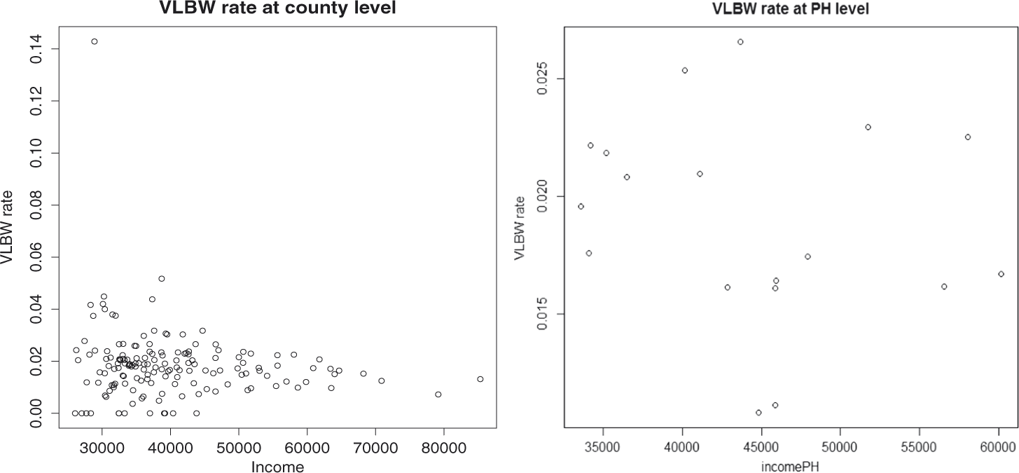Since % of poverty is highly correlated with income ( $\overset{\land}{ρ} = - 0.845$ and $\overset{\land}{ρ} = - 0.836$ at the county and PH levels, respectively), it can be used as an IV to estimate the ME variance.

The spatial pattern of the observed VLBW rate (incidence) and the median household income at both the county and PH levels is shown in Figure 1. We can see that there is an inverse relationship between income and VLBW incidence (Figure 2). There are high VLBW incidences at the central and southwest of the GA state, whereas the associated median household income is relatively low in those areas. Furthermore, the observed income has a spatial structure. We describe this spatial dependency of the error-contaminated income (W) through the PCAR structure (see Model 1; Section 3.1). In practice, the ME could be spatially dependent. For example, the error associated with household-reported income could be high for areas which have wealthy residents, whereas it could be low for areas which have poor residents. The analysis of this data set accounting for both ME and scale effect is deferred to Section 4.

Figure 1.

Observed very low birth weight (VLBW) incidence at the county and PH levels (top figure) and median household income at the county and PH levels (bottom figure). In this figure as well as in the subsequent figures, the second bracketed values are the number of regions in each risk category.

Figure 2.

The relationship between income and VLBW rate at the county and PH levels.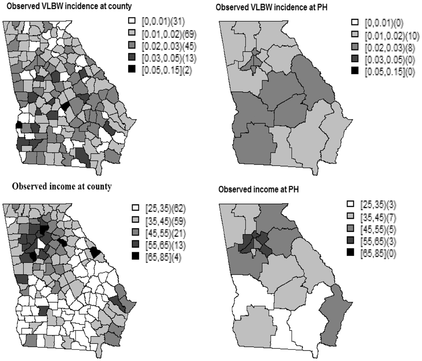

3 Multiscale ME models

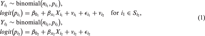
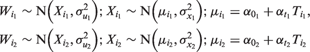
The goal of this paper is to model explicitly the spatially dependent predictor using ME in the multiscale modeling framework. Suppose $Y i k$ is the outcome random variable for the region $i; i k = 1, \dots, N k$ , at the scale level $k; k = 1, 2, \dots, K$ , N_k is the number of regions at the scale level k, and K is the total number of scale levels. Furthermore, assume $X i k$ is the unobserved variable of interest, and $W i k$ is the corresponding observed error-contaminated variable, and $Z_{i k}^{T}$ is the vector of p other covariates measured without error for geographical area i at the k^th scale level. Conditioning on the spatially structured random effect $v i k$ , we assume that the outcomes $Y i k$ are independent with densities $f (y i k | v i k, β x k, \underline{β} z k; μ i k)$ with $h (μ i k) = β 0 k + β x k X i k + Z_{i k}^{T} \underline{β} z k + v i k + ε i k$ for a known link function h, such as, identity, logit, and log link for continuous, binomial, and count data, respectively. The unstructured random effect $ε i k$ is $N (0, σ_{\in k}^{2})$ , and $v i k$ is assumed to have an ICAR structure. Since the predictor $X i k$ is unobserved, it can be estimated using functional and structural modeling. In the classical ME, $W i k$ and $X i k$ can be linked as $W i k = X i k + U i k$ , where the ME $U i k$ is $N (0, σ_{u k}^{2})$ and assumed to be independent of the unobserved true predictor $X i k$ . Alternatively, we can assume that the ME is spatially dependent and a PCAR structure can be used. To our knowledge, assuming a PCAR for the ME has never been explored before. Hence, in this paper, we focus to compare the performance of PCAR and normal distribution assumptions for the ME.

The ME variance can be estimated using replicate measurements or validation data. However, it is not always possible to get replication measurements or validation data. In such cases, an IV, T, can be used to estimate the regression model parameters.³ In this paper, we use an IV to estimate the parameters. Hence, the regression of $X i k$ on $(Z_{i k}^{T}, T i k)$ has mean $α 0 k + Z_{i k}^{T}$ $\underline{α} z k + α t k T i k$ . The true unobserved covariate $X i k$ , which is the mean of the error-contaminated covariate $W i k ~ N (X i k, σ_{u k}^{2})$ , is estimated using the observed variables $T i k$ and $Z_{i k}^{T}$ . If we estimate $X i k$ by borrowing information from $T i k$ and $Z_{i k}^{T}$ , intuitively, we can estimate the ME variance $σ_{u k}^{2}$ using the observed values of $W i k$ and the estimated values of $X i k$ . In other words, we need an IV to estimate $σ_{x k}^{2} = var (X i k)$ . Thereafter, the ME variance $σ_{u k}^{2}$ is estimated using $var (W i k)$ and $σ_{x k}^{2}$ . In general, all the parameters are identified because they are function of the moments of the observed variables.²⁴ Using the IV $T i k$ , Carroll et al.²⁴ have shown that the regression coefficients can be estimated as follows: $α t k = cov (Y i k, T i k) / cov (Y i k, W i k)$ and $α 0 k = E (T i k - α t k W i k)$ . In the next section, we present our models starting from the most complex method that accounts for the scaling effect and the ME simultaneously. Later, we present the naive multiscale model that ignores the ME as well as the scaling effect.

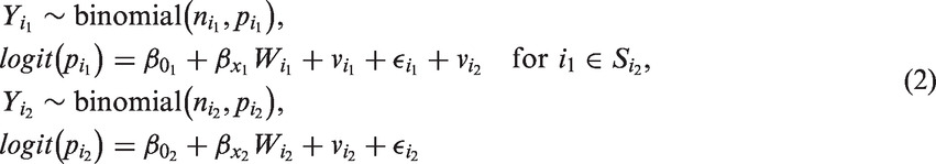
3.1 Model 1

We demonstrate here the spatial multiscale ME model for binomial data obtained from two scale levels, i.e., k = 1, 2. Let $Y i 1, Y i 2, n i 1$ , and $n i 2$ be the outcome random variables and the number of trials at the subunit (finer) and unit (coarser) levels, respectively. Furthermore, assume that $X i 1, X i 2, W i 1, W i 2, T i 1$ , and $T i 2$ are the true unobserved covariates, the observed error-contaminated covariates, and the IVs at the unit and subunit levels, respectively. In this paper, we only study the relationship between $Y i k$ and $X i k$ , where k = 1, 2. Our methods can be easily extended when there are error-free covariates, $Z_{i k}^{T}$ . The multiscale ME model that accounts for ME and scaling effect is given by

Y i 1 ~ binomial (n i 1, p i 1), logit (p i 1) = β 01 + β x 1 X i 1 + v i 1 + ε i 1 + v i 2 for i 1 \in S i 2, Y i 2 ~ binomial (n i 2, p i 2), logit (p i 2) = β 02 + β x 2 X i 2 + v i 2 + ε i 2

(1)

Here,

p i 1

and

p i 2

are the incidence of a disease at subunit (subregion)

i 1 = 1, 2, \dots, N 1

and unit (region)

i 2 = 1, 2, \dots, N 2

, where N₁ and N₂ are the number of subunit and unit levels, respectively. Furthermore,

S i 2

denotes the set of subunits at the finer level within the coarser level. Note that we link the two levels through a shared correlated random effect

v i 2

that allows to share common characteristics between the subunits within a unit level. The shared random effect handles the scaling effect. We assumed a normal distribution for the uncorrelated random effects

ε i k ~ N (0, σ ε k)

with k = 1, 2 and ICAR structure for the correlated random effects

v i k

, where k = 1, 2, given by

v i k | v - i k ~ N (\bar{v} δ i k, \frac{σ_{v k}^{2}}{n δ i k})

Here

\bar{v} δ i k = \frac{1}{n δ i k} \sum_{j ε δ i k} v j k

where

n δ i k

is the number of neighbors at subunit k = 1 and unit k = 2 levels and

δ i k

is the set of labels of the neighbors of unit i for scale level k. Note that we can have subunits be neighbors even if they have different parents (units). Neighbors are those regions that share a common boundary,¹ and in this paper, they are defined based on the adjacency-matrix.

We have seen that the shared correlated random effect handles the scaling effect. To accommodate for the ME, we used a PCAR structure. The PCAR formulation for the error-contaminated covariate $W i 1$ at the subunit (subregion) level is given by

[W i 1 | \dots] ~ N (X i 1, σ_{u 1}^{2} / n δ i 1); X i 1 ~ N (μ i 1, σ_{x 1}^{2}); μ i 1 = r i 1 + φ 1 \sum_{j \in δ i 1} (W j 1 - r j 1) / n δ i 1

Similarly, PCAR for the ME at the unit level is expressed as

[W i 2 | \dots] ~ N (X i 2, σ_{u 2}^{2} / n δ i 2); X i 2 ~ N (μ i 2, σ_{x 2}^{2}); μ i 2 = r i 2 + φ 2 \sum_{j \in δ i 2} (W j 2 - r j 2) / n δ i 2

where

φ i 1

and

φ i 2

are the correlation parameters, while

r i 1

and

r i 2

are the trends at the subregion and region levels written as

r i 1 = α 01 + α t 1 T i 1

and

r i 2 = α 02 + α t 2 T i 2

, respectively. Note that

σ_{x 1}^{2}, σ_{x 2}^{2}, σ_{u 1}^{2}

, and

σ_{u 2}^{2}

represent the variances of

X i k

with k = 1, 2 and the ME variances at the subunit and unit levels, respectively. Finally, we assumed non-informative normal priors for the regression coefficients and uniform priors, U(0, 100), for the standard deviations.²⁵

3.2 Model 2

Model 1 assumes a spatially dependent ME. In the literature, the ME is often assumed to be normally distributed.²⁶ This assumption could be used when the ME does not have a spatial structure. Hence, in this model, we assumed the ME follows a normal distribution. The model formulation for aggregated data at the unit and subunit levels is similar with Model 1 in equation (1) except now $W i 1$ and $W i 2$ are given by

W i 1 ~ N (X i 1, σ_{u 1}^{2}); X i 1 ~ N (μ i 1, σ_{x 1}^{2}); μ i 1 = α 01 + α t 1 T i 1, W i 2 ~ N (X i 2, σ_{u 2}^{2}); X i 2 ~ N (μ i 2, σ_{x 2}^{2}); μ i 2 = α 02 + α t 2 T i 2

We assumed similar prior distributions for the model parameters as in Model 1.

3.3 Model 3

Models 1 and 2 address both the scaling effect and the ME simultaneously. In this section, our interest is to address only the scaling effect. This approach could help us to investigate the effect of ignoring ME in the framework of multiscale modeling. The multiscale model that accounts for the scaling effect alone but not for the ME is defined as

Y i 1 ~ binomial (n i 1, p i 1), logit (p i 1) = β 01 + β x 1 W i 1 + v i 1 + ε i 1 + v i 2 for i 1 \in S i 2, Y i 2 ~ binomial (n i 2, p i 2), logit (p i 2) = β 02 + β x 2 W i 2 + v i 2 + ε i 2

(2)

Here also, we assumed similar prior distributions for the model parameters as in Model 1.

3.4 Model 4

In the previous section, we have seen models (Models 1 and 2) that address both the scaling effect and the ME. Also, we described a model (Model 3) that accommodates the scaling effect but not the ME. To assess the impact of ignoring both the scale effect and the ME, we describe here the simple naive approach. The model is of the form

Y i 1 ~ binomial (n i 1, p i 1), logit (p i 1) = β 01 + β x 1 W i 1 + v i 1 + ε i 1, Y i 2 ~ binomial (n i 2, p i 2), logit (p i 2) = β 02 + β x 2 W i 2 + v i 2 + ε i 2

(3)

Note that there is no random effect that introduces linkage between the two levels, and hence it ignores the scale effect. Furthermore, we are using the error-contaminated covariate $W i k$ in the model without adjusting for the ME. Hence, Model 4 neither accounts for scaling effect nor for ME.

3.5 Model assessment and selection

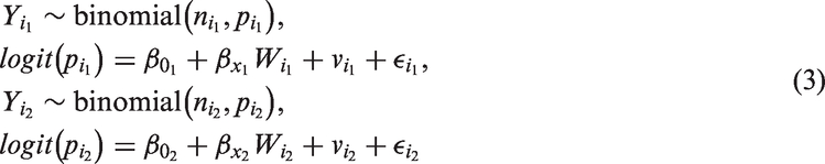
We compared the performance of the models using different criteria and prediction accuracy measurements. For the model selection, we employed a deviance information criterion²⁷ (DIC) and a Watanabe–Akaike information criterion (WAIC).²⁸ The DIC is a combination of the deviance and the effective number of parameters (PD) that penalizes for model complexity, while the WAIC is an approximation to cross-validation. In addition, the DIC is not a fully Bayesian method as it is based on a point estimate,^29,30 whereas the WAIC is a fully Bayesian technique and uses a posterior distribution. To measure the predictive ability of the models, we implemented the mean square prediction error (MSPE) and mean absolute prediction error (MAPE) given by

MSPE = \frac{1}{N k \times G} \sum_{j = 1}^{G} \sum_{i = 1}^{N k} (y i k - y_{i k, j}^{pred})^{2} MAPE = \frac{1}{N k \times G} \sum_{j = 1}^{G} \sum_{i = 1}^{N k} | y i k - y_{i k, j}^{pred} |

where

y_{i k, j}^{pred}

and N_k are the predicted values of the outcome for region i and the number of spatial units at scale level k, respectively. Note that G denotes the posterior sample size.

The models were applied in real and simulated data (see Sections 4 and 5) using the mix of Gibbs and Metropolis–Hastings algorithms of Markov chain Monte Carlo (MCMC) via R2WinBUGS package (see online Supplementary Appendix).

4 Simulation study

The aim of the simulation study is the following: (1) to investigate the impact of ignoring ME and scaling effect for multiscale spatial data, (2) to study the benefit of accounting for ME and scaling effect, and (3) to compare the performance of using a normal distribution and a PCAR for spatially dependent ME. We considered two scenarios: (1) we assumed an independent ME and (2) a spatially structured ME. We describe each scenario in the next section.

4.1 Scenario 1: An independent ME

Many studies assume independent ME in predictors. This is less reasonable for spatial data. In such cases, we can still use Model 1 that assumes a spatially dependent ME because $φ l 1$ described in Section 3 will be zero, and Model 1 is simplified to Model 2 which assumes an independent ME. Our interest here is to assess the impact of using a spatially dependent ME for data simulated from an independent ME. We expect the spatially dependent ME will provide similar results as the model that assumes an independent ME. Hence, we simulated data within the Georgia state map assuming an independent normal distribution, $U l 1 ~ N (0, σ_{u 1}^{2})$ , from the following model

y l 1 ~ binomial (n l 1, p l 1), logit (p l 1) = β 01 + β x 1 X l 1 + v l 1 + ε l 1

(4)

where

l 1 = 1, \dots, 159, n l 1

is the sample size in each county, and it is generated from a multinomial distribution,

n l 1 ~ Multinomial (n, N l 1 / N)

for which

N l 1

is the population size in each county and N is the total population size in the state of Georgia in 2007. We assumed n to be fixed and equal to 50,000. The true covariate

X l 1

is assumed to represent the median household income (in thousands) in the US. We simulated a spatial structure

X l 1

using a Matérn correlation function (see online Supplementary Appendix). Since we simulated

X l 1

and

U l 1

, it is a straightforward now to generate the error-contaminated covariate

W l 1

as follows:

W l 1 = X l 1 + U l 1

. Similar in Carroll et al.,³ we simulated the IV as

T l 1 ~ N (α 01 + α 11 X l 1, σ_{t 1}^{2})

. The simulated values for

X l 1, W l 1, T l 1

, and

U l 1

at the county level are shown in Figure 3.

Figure 3.

Generated true covariate (X), error-prone covariate (W), instrumental variable (T), and measurement error (U) for the counties of Georgia (scenario 1).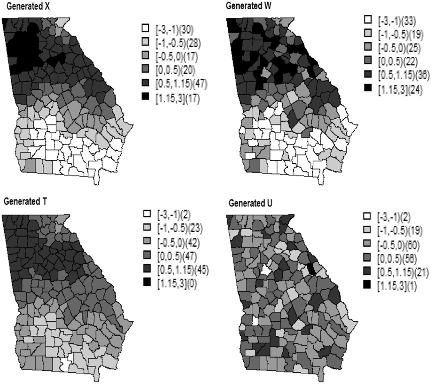

To obtain $X i 2, W i 2$ , and $T i 2$ at the PH level, we averaged the simulation values of the counties within the given PH district, i.e., $X i 2 = \sum_{l 1 \in S i 2} X l 1 / n S i 2, W i 2 = \sum_{l 1 \in S i 2} W l 1 / n S i 2$ and $T i 2 = \sum_{l 1 \in S i 2} T l 1 / n S i 2$ , where $i 2 = 1, \dots, 18$ , and $n S i 2$ is the number of counties within a PH district. Similarly, the outcome $y i 2$ and the number of trials at each PH district $(n i 2)$ were obtained by summing up the outcome and the number of trials of the counties within the given PH district, i.e., $y i 2 = \sum_{l 1 \in S i 2} y l 1$ and $n i 2 = \sum_{l 1 \in S i 2} n l 1$ . Finally, we considered the ICAR-distribution to generate the spatially structured random effect $v l 1$ and a normal distribution with mean 0, and variance $σ_{ε 1}^{2}$ was used to obtain the noise term $ε l 1$ .

4.2 Scenario 2: A spatially structured ME

Since we are interested in modeling ME for spatial data, it is more reasonable to assume a spatial dependent ME. Here, we investigate the misspecification of the ME, i.e., the impact of assuming an independent ME for data simulated using a spatially structured ME. Hence, we simulated the ME $U l 1$ as well as $X l 1$ using the Matérn correlation function (see online Supplementary Appendix). We simulated $W l 1$ as $W l 1 = X l 1 + U l 1$ and $T l 1$ as $T l 1 ~ N (α 01 + α 11 X l 1, σ_{t 1}^{2})$ . The covariates $X i 2, W i 2$ , and $T i 2$ at the PH level were computed as we mentioned in scenario 1. The simulated values for the covariates at the county level are shown in Figure 4. Comparing Figures 3 and 4, the error-prone covariate $W l 1$ and the ME $U l 1$ obtained from scenario 2 are more spatially structured than those obtained from scenario 1. In both scenarios 1 and 2, we simulated 200 data sets, and we fitted the Models 1–4 discussed in Section 3.

Figure 4.

Generated true covariate (X), error-prone covariate (W), instrumental variable (T), and measurement error (U) for the counties of Georgia (scenario 2).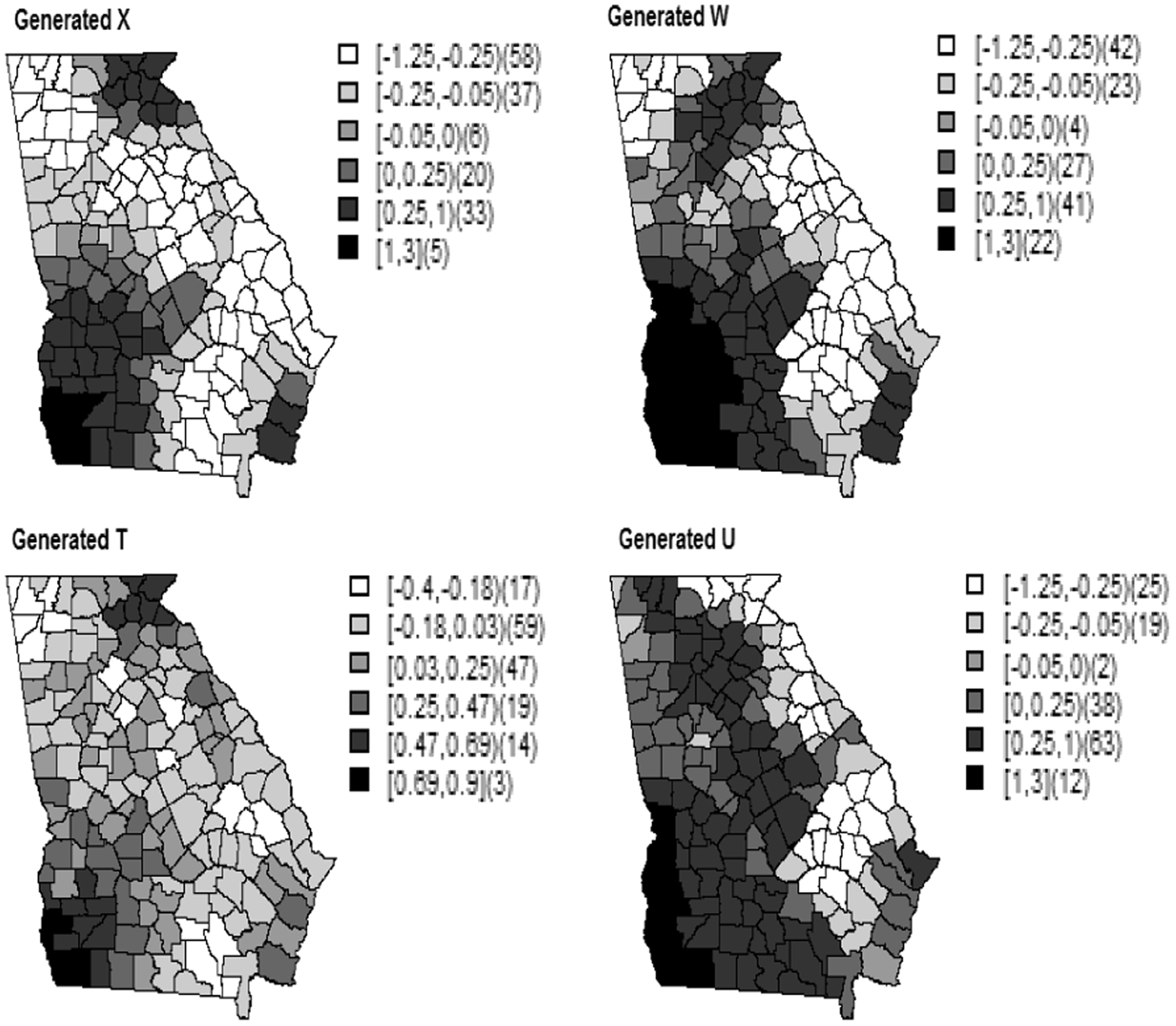

4.3 Simulation results

4.3.1 Scenario 1: An independent ME

The results of the model fit with and without accounting for the ME and the scale effect are displayed in Table 1, indicating that Model 1 fits as good as Model 2. Furthermore, both Models 1 and 2 fit better than Models 3 and 4 at the county level as measured by DIC. Also, Models 1 and 2 have the smallest effective number of parameters (PD). This shows that the models that allow an ME describe the risk variation better than the models that ignore the ME. The prediction accuracy from all the models is similar. To investigate the impact of ignoring the ME, we calculated the parameter estimates as shown in Table 2 and the coverage of the 95% credible interval (CI) as displayed in Table 3. As expected, the naive models that ignore the ME (Models 3 and 4) underestimate the slope parameter

β x 1

of the true unobserved predictor. On the other hand, the models that take into account both the ME and the scale effect result in an unbiased estimate for

β x 1

. Also, the naive models yield an inflated estimate for the variance of the spatially structured component

(σ_{v 1}^{2})

. These results are similar with the results obtained for spatial univariate data in Li et al.²⁶ Note that θ₁ in Tables 1 and 4 denotes the relative risk at county level. The bias and mean square error (MSE) of this relative risk were obtained by averaging over the 200 simulated data sets and 159 counties.

Table 1.

Simulation results for data generated within the Georgia state map.

	PD_dic		DIC		PD_waic		WAIC		MAPE		MSPE		θ ₁
Models	County	PH district	County	PH district	County	PH district	County	PH district	County	PH district	County	PH district	Bias	MSE
Model 1	62.89	13.48	1073.27	181.4	45.75	8.96	1071.31	178.13	7.74	27.96	144.39	1291.16	−0.58	0.338
Model 2	61.42	15.63	1072.74	181.36	47.16	8.93	1071.12	178.08	7.75	27.94	144.46	1290.82	−0.58	0.338
Model 3	81.62	16.54	1082.57	181.25	53.95	8.98	1071.31	178.14	7.67	27.94	144.43	1290.28	−0.58	0.339
Model 4	80.98	16.32	1083.16	181.98	54.21	8.94	1072.84	178.05	7.68	27.94	144.67	1290.35	−0.58	0.339

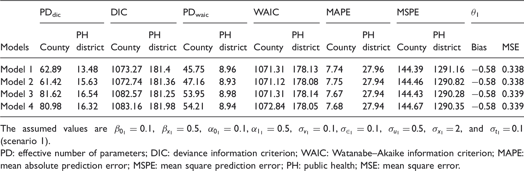
The assumed values are $β 01 = 0.1$ , $β x 1 = 0.5$ , $α 01 = 0.1, α 11 = 0.5$ , $σ v 1 = 0.1, σ \in 1 = 0.1$ , $σ u 1$ = 0.5, $σ x 1$ = 2, and $σ t 1$ = 0.1 (scenario 1).

PD: effective number of parameters; DIC: deviance information criterion; WAIC: Watanabe–Akaike information criterion; MAPE: mean absolute prediction error; MSPE: mean square prediction error; PH: public health; MSE: mean square error.

Table 2.

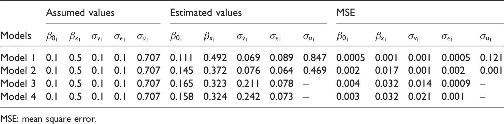
Summary of the estimated values and MSE of the parameters for the data generated within the Georgia state map (scenario 1).

	Assumed values					Estimated values					MSE
Models	$β 01$	$β x 1$	$σ v 1$	$σ \in 1$	$σ u 1$	$β 01$	$β x 1$	$σ v 1$	$σ \in 1$	$σ u 1$	$β 01$	$β x 1$	$σ v 1$	$σ \in 1$	$σ u 1$
Model 1	0.1	0.5	0.1	0.1	0.5	0.114	0.489	0.071	0.083	0.447	0.0003	0.0006	0.001	0.0007	0.003
Model 2	0.1	0.5	0.1	0.1	0.5	0.114	0.488	0.067	0.065	0.421	0.0003	0.0006	0.001	0.002	0.006
Model 3	0.1	0.5	0.1	0.1	0.5	0.116	0.150	0.343	0.051	–	0.0005	0.123	0.059	0.003	–
Model 4	0.1	0.5	0.1	0.1	0.5	0.1037	0.153	0.357	0.051	–	0.0002	0.121	0.067	0.003	–

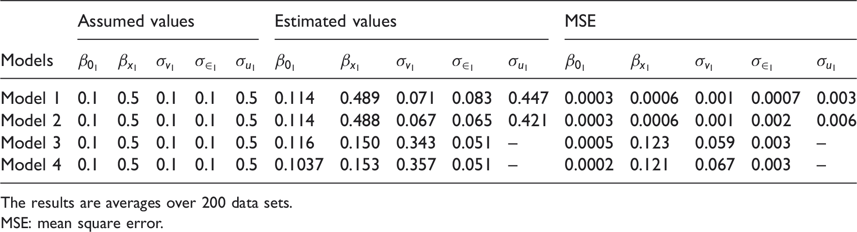
The results are averages over 200 data sets.

MSE: mean square error.

Table 3.

Simulation study.

	Assumed values					Coverage (%)
Models	$β 01$	$β x 1$	$σ v 1$	$σ ε 1$	$σ u 1$	$β 01$	$β x 1$	$σ v 1$	$σ ε 1$	$σ u 1$
Model 1	0.1	0.5	0.1	0.1	0.5	100	100	100	97.5	45.5
Model 2	0.1	0.5	0.1	0.1	0.5	98.5	100	97.5	97	41.0
Model 3	0.1	0.5	0.1	0.1	0.5	91.5	0.0	0.0	94.0	–
Model 4	0.1	0.5	0.1	0.1	0.5	97.0	0.0	0.0	91.0	–

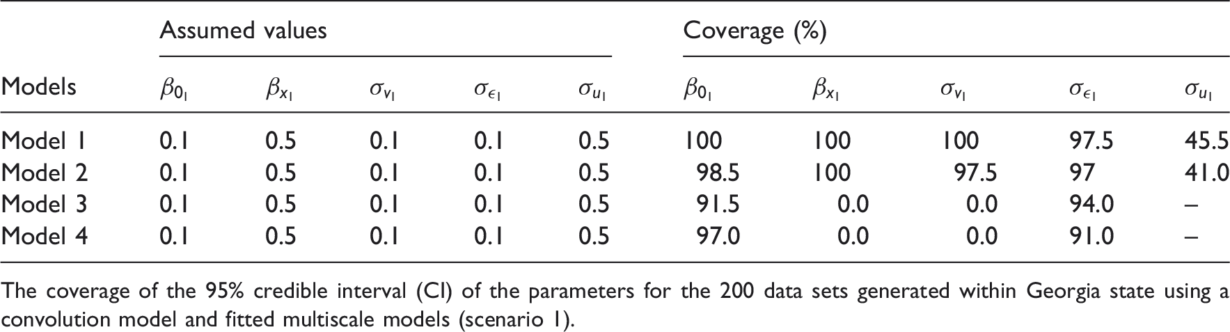
The coverage of the 95% credible interval (CI) of the parameters for the 200 data sets generated within Georgia state using a convolution model and fitted multiscale models (scenario 1).

Table 4.

Simulation results for data generated within the Georgia state map.

	PD_dic		DIC		PD_waic		WAIC		MAPE		MSPE		θ ₁
Models	County	PH district	County	PH district	County	PH district	County	PH district	County	PH district	County	PH district	Bias	MSE
Model 1	57.24	13.08	1074.30	179.16	45.71	8.30	1074.75	177.43	7.95	28.39	152.42	1330.24	−0.55	0.304
Model 2	58.81	14.68	1076.45	180.57	47.16	8.43	1075.85	178.79	7.92	28.45	152.08	1335.82	−0.55	0.304
Model 3	68.79	14.74	1081.48	180.96	50.89	8.52	1078.05	177.93	7.91	28.51	152.31	1347.39	−0.55	0.304
Model 4	70.01	15.63	1080.15	182.12	50.46	8.88	1075.07	178.74	7.88	28.59	152.18	1355.38	−0.55	0.304

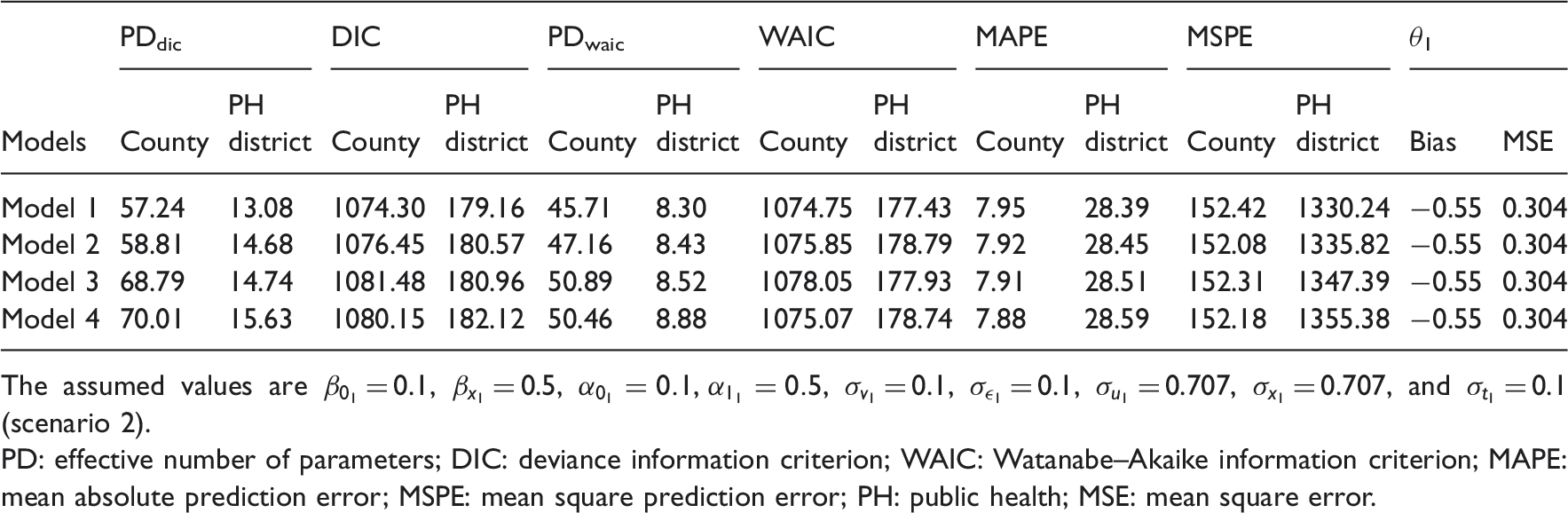
The assumed values are $β 01$ = 0.1, $β x 1$ = 0.5, $α 01 = 0.1, α 11 = 0.5$ , $σ v 1$ = 0.1, $σ ε 1$ = 0.1, $σ u 1$ = 0.707, $σ x 1$ = 0.707, and $σ t 1$ = 0.1 (scenario 2).

Table 5.

Summary of the estimated values and MSE of the parameters for the data generated within the Georgia state map (scenario 2).

	Assumed values					Estimated values					MSE
Models	$β 01$	$β x 1$	$σ v 1$	$σ ε 1$	$σ u 1$	$β 01$	$β x 1$	$σ v 1$	$σ ε 1$	$σ u 1$	$β 01$	$β x 1$	$σ v 1$	$σ ε 1$	$σ u 1$
Model 1	0.1	0.5	0.1	0.1	0.707	0.111	0.492	0.069	0.089	0.847	0.0005	0.001	0.001	0.0005	0.121
Model 2	0.1	0.5	0.1	0.1	0.707	0.145	0.372	0.076	0.064	0.469	0.002	0.017	0.001	0.002	0.001
Model 3	0.1	0.5	0.1	0.1	0.707	0.165	0.323	0.211	0.078	–	0.004	0.032	0.014	0.0009	–
Model 4	0.1	0.5	0.1	0.1	0.707	0.158	0.324	0.242	0.073	–	0.003	0.032	0.021	0.001	–

MSE: mean square error.

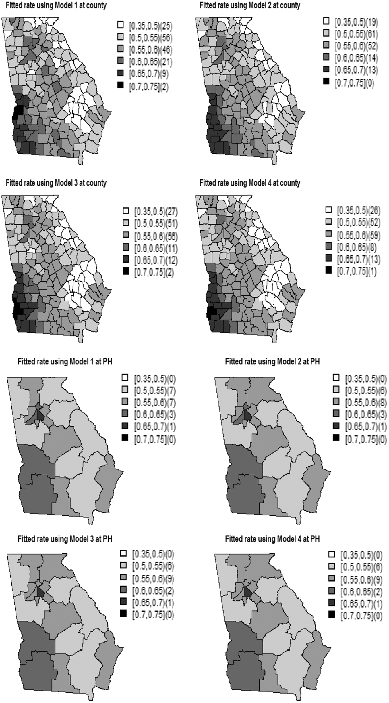
Furthermore, the coverage of the 95% CI for regression coefficient $β x 1$ and the spatially structured variance component $σ_{v 1}^{2}$ obtained from the naive models (Models 3 and 4) is zero. This is not surprising because the naive models provide highly bias and unprecise estimates for these parameters as shown in Table 2. On the other hand, the model that assumes a spatially structured ME provides 100% coverage for these parameters. However, the 95% coverage probability for the ME variance $σ_{u 1}^{2}$ is below 50% for the models that account for the ME as well as the scale effect (Models 1 and 2). Yet, the estimate of the ME variance is not highly biased; the assumed value for the ME variance was 0.5, and the estimated variance from Models 1 and 2 is approximately 0.45 and 0.42, respectively.

To investigate how well the models recover the risk variation, we compared the generated risks and the risks obtained from the models as shown in Figures 5 and 6, respectively. We can see that all the models recover well the generated risk variation. There is a slight difference between the models in terms of recovering the risk variation.

Figure 5.

Simulation study. Generated risks at each county ( $p l 1 = expit (β 01 + β 11 \times X l 1 + v l 1 + ε l 1)$ ; left panel) and average of generated risks of the counties within the given public health (PH) district (right panel) (scenario 1).

Figure 6.

Simulation study. Average of the risks obtained from the models fitted to the 200 data sets generated within the Georgia state (scenario 1).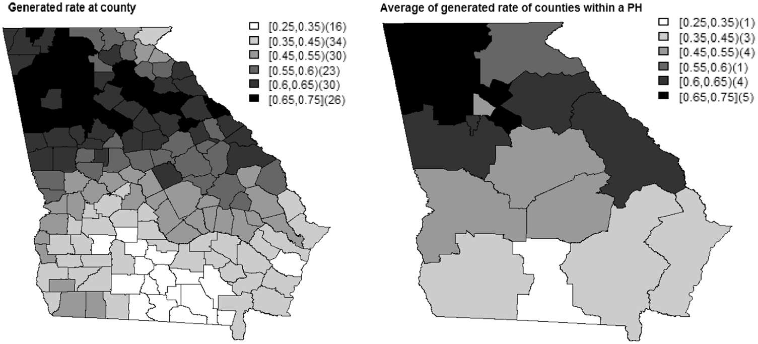

4.3.2 Scenario 2: A spatial structured ME

The results obtained from Models 1–4 fitted to the simulated data sets assuming a spatially structured ME are shown in Tables 4 to 6. Using the DIC and WAIC, Model 1 slightly outperforms the other models at both the county and PH levels. Also, Model 1 produces a better prediction accuracy and the smallest number of effective parameters as compared to the other models at the PH level. The parameter estimates and the coverage of the 95% CI obtained from Model 1 indicate that Model 1 provides more unbiased and precise estimates for all the model parameters as compared to the other models. However, using an independent ME for the data simulated assuming a spatially dependent ME results in a biased estimate of the regression coefficient associated with the true covariate

X l 1

(β x 1)

as well as the ME variance

σ_{u 1}^{2}

. As in scenario 1, ignoring the ME underestimates

β x 1

and inflates the variance of the spatially structured random effect

σ_{v 1}^{2}

. In contrast to scenario 1, ignoring the ME here results in a bias and a bad coverage of the 95% CI for the intercept parameter

β 01

Table 6.

Simulation study.

	Assumed values					Coverage (%)
Models	$β 01$	$β x 1$	$σ v 1$	$σ ε 1$	$σ u 1$	$β 01$	$β x 1$	$σ v 1$	$σ ε 1$	$σ u 1$
Model 1	0.1	0.5	0.1	0.1	0.707	100	100	100	97.5	95.0
Model 2	0.1	0.5	0.1	0.1	0.707	46.5	18.5	100	89.0	56.5
Model 3	0.1	0.5	0.1	0.1	0.707	0	0	98	92.5	–
Model 4	0.1	0.5	0.1	0.1	0.707	0	0	45.5	82.0	–

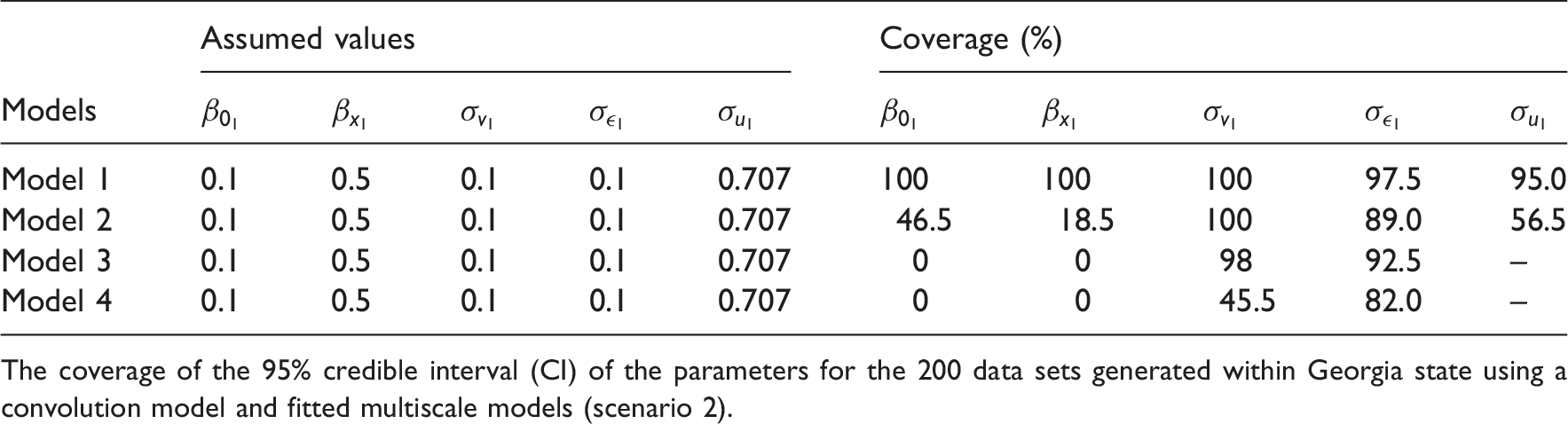
The coverage of the 95% credible interval (CI) of the parameters for the 200 data sets generated within Georgia state using a convolution model and fitted multiscale models (scenario 2).

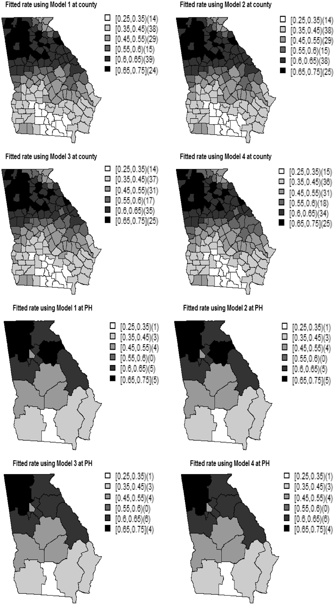
Figures 7 and 8 show the simulated risk, and the estimated risks are obtained from Models 1–4, respectively. We can see that Model 1 recovers the risk variation at the county and PH levels slightly better than the other models. For example, both the simulated and the estimated risks obtained from Model 1 are relatively low to the northeast of Georgia at the PH district, whereas the other models provide a relatively higher risk in those areas.

Figure 7.

Figure 8.

Simulation study. Average of the risks obtained from the models fitted to the 200 data sets generated within the Georgia state (scenario 2).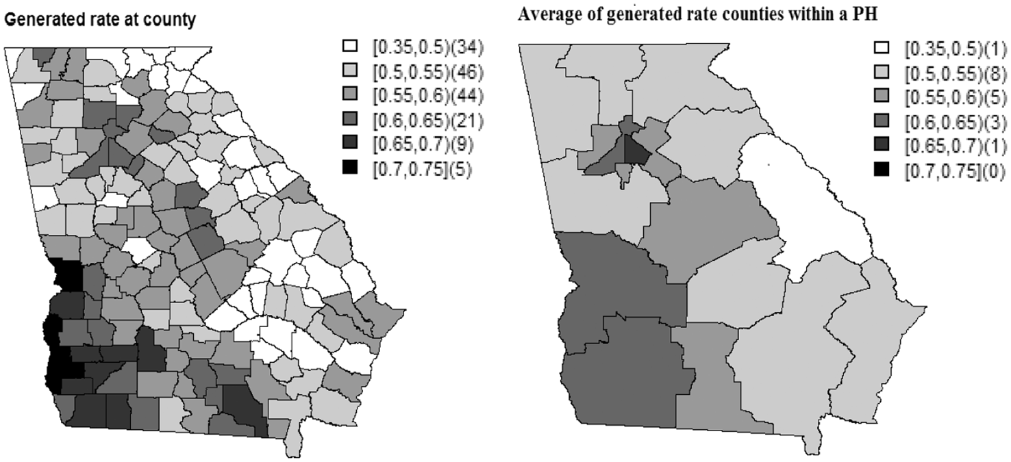

5 Application to Georgia VLBW incidence

We fitted the models using MCMC. To improve convergence, the covariates income and poverty were standardized. The scale reduction factor (

\overset{\land}{R}

was equal to one for all the parameters) and trace plots suggest that convergence has achieved for all the model parameters. The results using Models 1–4 are shown in Tables 7 and 8. We can see that accounting for both ME and scale effect (Models 1 and 2) simultaneously improves the model fit at the county level as compared to Model 3 that accounts for the scaling effect alone and Model 4, which ignores both the ME and scaling effect, at both the county and PH levels. Although it is not significant, assuming a spatially dependent ME (Model 1) slightly improves the model fit and prediction accuracy as compared to the model that assumes an independent ME (Model 2). Furthermore, the penalty value (PD) obtained from Model 1 is the smallest one as compared to the other models. Hence, Model 1 provides a better description of the disease risk variation as compared to the other models. The predictive accuracy is similar for Models 1–3, whereas Model 4 has the worst predictive accuracy at the PH level. The shared multiscale model with ME results in a better model fit than without the ME. On the other hand, sharing the correlated component alone (Model 3) improves the model fit and prediction accuracy as compared to the independent multiscale model (Model 4).

Table 7.

Model fit and predictive accuracy results for Georgia VLBW data.

	PD_dic		DIC		PD_waic		WAIC		MAPE		MSPE
Models	County	PH district	County	PH district	County	PH district	County	PH district	County	PH district	County	PH district
Model 1	18.96	10.83	765.71	145.98	15.39	4.84	764.39	141.06	3.56	12.64	33.04	266.3
Model 2	20.09	11.18	766.56	146.12	16.39	4.76	765.16	141.41	3.56	12.61	33.07	267.0
Model 3	20.22	11.23	773.49	146.17	17.95	4.72	774.45	142.23	3.61	12.6	33.8	265.8
Model 4	46.13	16.10	782.62	155.58	33.53	8.83	778.02	151.63	3.54	13.5	34.36	301.5

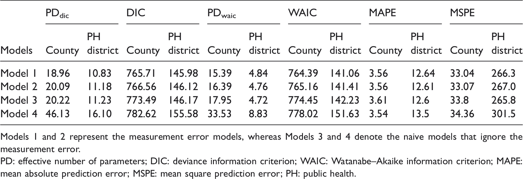
Models 1 and 2 represent the measurement error models, whereas Models 3 and 4 denote the naive models that ignore the measurement error.

Table 8.

Georgia VLBW incidence data.

	Mean												SD
Models	$β 01$	$β 02$	$β x 1$	$α t 1$	$β x 2$	$α t 2$	$σ v 1$	$σ ε 1$	$σ u 1$	$σ v 2$	$σ ε 2$	$σ u 2$	$β 01$	$β 02$	$β x 1$	$α t 1$	$β x 2$	$α t 2$	$σ v 1$	$σ ε 1$	$σ u 1$	$σ v 2$	$σ ε 2$	$σ u 2$
Model 1	−3.97	−3.971	−0.164^a	−0.851^a	−0.123^a	−0.852^a	0.262	0.127	1.1	0.341	0.132	1.136	0.033	0.045	0.047	0.041	0.065	0.158	0.089	0.057	0.075	0.155	0.083	0.431
Model 2	−3.919	−3.974	−0.174^a	−0.845^a	−0.129^a	−0.829^a	0.076	0.054	0.503	0.399	0.035	0.537	0.029	0.030	0.043	0.042	0.063	0.152	0.051	0.038	0.059	0.399	0.027	0.177
Model 3	−3.923	−3.975	−0.092^a	−	−0.061	–	0.067	0.063	–	0.445	0.032	–	0.029	0.023	0.029	–	0.038	–	0.052	0.042	–	0.096	0.027	–
Model 4	−3.979	−3.975	−0.097^a	–	0.005	–	0.283	0.141	–	0.371	0.119	–	0.033	0.039	0.034	–	0.076	–	0.084	0.052	–	0.145	0.085	–

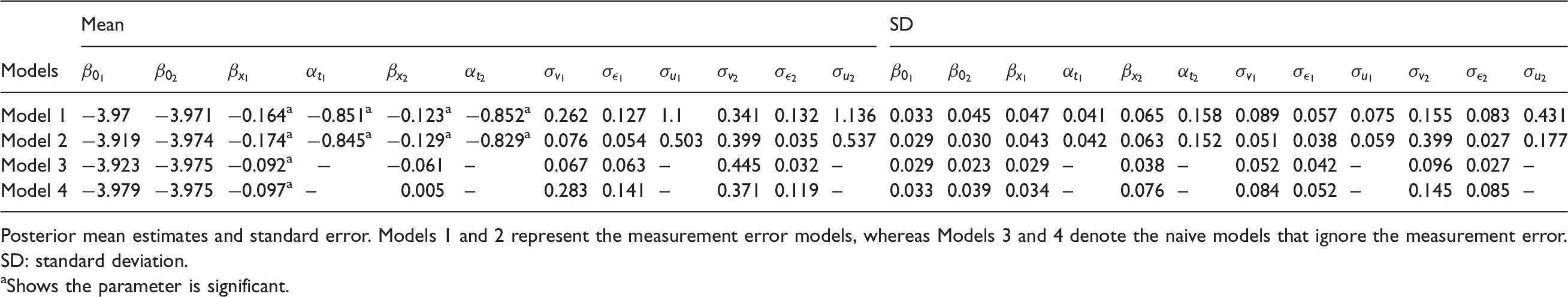
Posterior mean estimates and standard error. Models 1 and 2 represent the measurement error models, whereas Models 3 and 4 denote the naive models that ignore the measurement error.

SD: standard deviation.

Shows the parameter is significant.

If we consider the absolute value of the estimate of the regression coefficient $(| β x 1 |)$ , the naive estimates obtained from Models 3 and 4 are attenuated. Obviously, there is a bias–variance trade off because the standard errors from the ME models for $| β x 1 |$ are slightly higher than that of the naive estimates (Table 8). Another interesting result from the models is that the negative relationship between income and VLBW rate obtained from Models 3 and 4 at the county level $(β x 1)$ did not hold true at the PH level $(β x 2)$ because in the later case the 95% CI covers a zero value. However, when we allow the model to adjust for both the ME and the scale effect simultaneously (Models 1 and 2), we obtained a negative relationship between income and VLBW at both the county and PH levels.

One way to assess whether a given covariate can be used as an IV (T) to the true unobserved covariate (X) is that T and X should be significantly related.³ Since the % of poverty is significantly associated with income $(α t 1 and α t 2)$ , it is an appropriate to use it as an IV to estimate the ME variance. Furthermore, as we mentioned in Section 1, the IV must be an independent of Y − E(Y|X). To investigate this condition, we plotted the residual versus the IV poverty as shown in Figure 9, indicating that the IV is independent of Y − E(Y|X).

Figure 9.

Pearson residuals versus the standardized instrumental variable poverty at the county and PH levels for Model 1 (top figure) and Model 2 (bottom figure).

To compare the models in terms of explaining the disease risk variation, we computed the VLBW incidence as shown in Figure 10. We can see that there is a higher risk of VLBW incidence to the central and southwest GA as compared to the other regions.

Figure 10.

Probability of VLBW outcome obtained from Models 1–4 at the county level (top figure) and at the public health (PH) district level (bottom figure).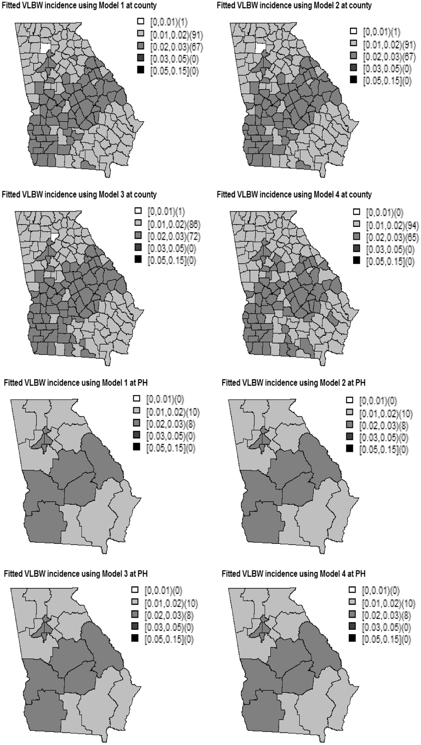

6 Discussion and conclusion

In this paper, our goal was to account for both ME and scale effect in our model-building for hierarchical multiscale spatial data, and we achieved this goal using multiscale classical ME models. We compared four models: the first two models (Models 1 and 2) accommodate the ME and the scale effect simultaneously. The third model (Model 3) only handles the scale effect. The fourth model (Model 4) ignores both the scale effect and the ME. The difference between the first two models (Models 1 and 2) is that Model 1 assumes a spatially dependent ME, whereas Model 2 assumes an independent ME. We evaluated the performance of the models in real and simulated data and found that accounting for both the ME and the scale effect improves the model fit as well as the prediction accuracy as compared to the model that ignores the ME and the scale effect (Model 4). Furthermore, the models that adjust for both the ME and the scale effect explain the risk variation better than the model that ignores both the ME and the scale effect. As it is the case for univariate data, we found that ignoring the ME for multiple scale data also underestimates the regression coefficient of the true unobserved covariate $(β x 1)$ . Evidently, we noticed from the simulation study that ignoring the ME inflates the spatially structured variance component $(σ v 1)$ , which is in line with the theoretical approximation and the simulation results obtained in Li et al.²⁶

When the outcome Y and the true unobserved covariate X share the same spatial variance components, it has been shown that ignoring the ME results in attenuated estimate of the regression coefficient and an inflated estimate of the spatial variance component. However, when the variance component of Y and X differ, no analytical expressions are available.²⁶ Note that our approach is different from the approach in Li et al.²⁶ because we assumed a PCAR for W, which is the proxy of X, whereas they²⁶ assumed the same variance component as in Y, i.e., $X i k = a 0 k + v i k + ε i k$ , where $v i k$ and $ε i k$ are the same as in Section 3.

Although we did not see a significant improvement in model fit and prediction accuracy for the VLBW incidence in Georgia, we found that the model that assumes a spatially dependent ME (Model 1) is slightly better than the model that assumes a spatially unstructured ME (Model 2). We also conducted a focused simulation study and obtained that Model 1 provides slightly better model fit and prediction accuracy than Model 2. Furthermore, Model 1 explains the risk variation slightly better than Models 2–4. Moreover, Model 1 provides more unbiased and precise estimates for the regression coefficient $(β x 1)$ as compared to Model 2. When we applied Model 2 for data simulated assuming a spatially dependent ME, we obtained biased estimates of $β x 1$ and $σ u 1$ (the ME variance).

There are several advantages of jointly modeling the risk variation at different geographical levels using a shared multiscale model after adjusting for ME. It results in a consistent negative effect of income on VLBW at both the county and PH levels. Accounting for the scale effect alone or ignoring both the ME and the scale effect, however, leads to inconsistent effect of income on VLBW incidence at the county and PH levels: While there is a significant negative effect of income on VLBW at the county level, we found insignificant income effect on VLBW at the PH level. Using Model 4, we obtained a negative effect of income on VLBW at the county level, whereas we obtained an insignificant positive effect of income on VLBW at the PH level. On the other hand, accounting for ME and scale effect provides unbiased estimate of the regression coefficient.

The models presented here only focus on the association between a response and an error-contaminated covariate. However, in the case of error-free covariates, our method could be extended as described in Section 3. Furthermore, we used a shared correlated random effect to jointly model the risk variation at different scale levels. Instead of sharing the correlated component, it is also possible to share the uncorrelated component or both the correlated and the uncorrelated random effects. In addition, we did not quantify the scale effect, and it can be done by assuming a multivariate PCAR or a multivariate normal distribution when the uncorrelated component is shared between the scale levels. In this paper, we conducted a focused simulation study to compare the models. An extensive simulation study that shows the importance of using a spatially structured ME remains our further research.

In summary, accounting for ME and scale effect due to data aggregation leads to a better description of disease risk variation than ignoring them. Moreover, the model fit and prediction accuracy obtained from the models that account for these two issues simultaneously are better than the parsimonious models. Ignoring the ME for multiscale data results in attenuation of bias and inconsistent estimate of the covariate effect at different scale levels. The methods proposed here are useful in health application and can be easily applied by health practitioners in standard software such as WinBUGS. Finally, we conclude that jointly modeling the disease risks at different geographical levels as well incorporating the ME for spatially aggregated data provides an accurate risk estimate that can be used for planning purpose.

Footnotes

Acknowledgements

The authors would like to acknowledge support from the National Institutes of Health via grant R01CA172805. The third author also acknowledges support from the IAP Research Network P7/06 of the Belgian State (Belgian Science Policy).

Declaration of conflicting interests

The author(s) declared no potential conflicts of interest with respect to the research, authorship, and/or publication of this article.

Funding

The author(s) received no financial support for the research, authorship, and/or publication of this article.

References

Besag

York

Mollié

. Bayesian image restoration with applications in spatial statistics (with discussion). Ann Inst Stat Math 1991; 43: 1–59.

Kolaczyk

Huang

. Multiscale statistical models for hierarchical spatial aggregation. Geogr Anal 2001; 33: 95–118.

Carroll

Ruppert

Stefanski

. Measurement error in nonlinear models: a modern perspective, 2nd ed. New York: Chapman and Hall/CRC, 2006.

Pierce

Kellerer

. Adjusting for covariate errors with nonparametric assessment of the true covariate distribution. Biometrica 2004; 91: 863–876.

Cook

Stefanski

. Simulation-extrapolation estimation in parametric measurement error models. J Am Stat Assoc 1994; 89: 1314–1328.

Carroll

Freedman

Hartman

. The use of semiquantitative food frequency questionnaires to estimate the distribution of usual intake. Am J Epidemiol 1996; 143: 392–404.

Devanarayan

Stefanski

. Empirical simulation extrapolation for measurement error models with replicate measurements. Stat Probab Lett 2002; 59: 219–225.

Vidakovic

. Statistical modeling by wavelets, New York: John Wiley, 1999.

Huang

Cressie

Gabrosek

. Fast, resolution-consistent spatial prediction of global processes from satellite data. J Comput Graph Stat 2002; 11: 63–88.

10.

Zhu

Yue

. A multiresolution tree-structured spatial linear model. J Comput Graph Stat 2004; 14: 168–184.

11.

Louie

Kolaczyk

. On the covariance properties of certain multiscale spatial processes. Stat Probab Lett 2004; 66: 407–416.

12.

Louie

Kolaczyk

. A multiscale method for disease mapping in spatial epidemiology. Stat Med 2006; 25: 1287–1306.

13.

Aregay

Lawson

Faes

. Bayesian multiscale modeling for aggregated disease mapping data. Stat Meth Med Res 2015. DOI: 10.1177/0962280215607546.

14.

Aregay

Lawson

Faes

. Impact of income on small area low birth weight incidence using multiscale models. AIMS Publ Health 2015; 2: 667–680.

15.

Molitor

Jerrett

Chang

. Assessing uncertainty in spatial exposure models for air pollution health effects assessments. Environ Health Perspect 2007; 115: 1147–1153.

16.

Zeger

Thomas

Dominici

. Exposure measurement error in time-series studies of air pollution: concepts and consequences. Environ Health Perspect 2000; 108: 419–426.

17.

Gryparis

Coull

Schwartz

. Semiparametric latent variable regression models for spatio-temporal modeling of mobile source particles in the greater Boston area. J Roy Stat Soc C 2009; 56: 183–209.

18.

Peng

Bell

. Spatial misalignment in time series studies of air pollution and health data. Biostatistics 2010; 11: 720–740.

19.

Gray

Gelfand

Miranda

. Hierarchical spatial modeling of uncertainty in air pollution and birth weight study. Stat Med 2011; 30: 2187–2198.

20.

Krieger

Chen

Waterman

. Choosing area based socioeconomic measures to monitor social inequalities in low birth weight and childhood lead poisoning: The Public Health Disparities Geocoding Project (US). J Epidemiol Community Health 2003; 57: 186–199.

21.

O’Campo

Xue

Wang

. Neighborhood risk factors for low birthweight in Baltimore: a multilevel analysis. Am J Public Health 1997; 87: 1113–1118.

22.

Roberts

. Neighborhood social environments and the distribution of low birthweight in Chicago. Am J Publ Health 1997; 87: 597–603.

23.

Parker

Schoendorf

Kiely

. Associations between measures of socioeconomic status and low birth weight, small for gestational age, and premature delivery in the United States. Ann Epidemiol 1994; 4: 271–278.

24.

Carroll

Ruppert

Crainiceanu

. Nonlinear and nonparametric regression and instrumental variables. J Am Stat Assoc 2004; 99: 736–750.

25.

Gelman

. Prior distribution for variance parameters in hierarchical models. Bayesian Anal 2006; 3: 515–533.

26.

Tang

Lin

. Spatial linear mixed models with covariate measurement errors. Statistica Sinica 2009; 19: 1077–1093.

27.

Spiegelhalter

Best

Carlin

. Bayesian measures of model complexity and fit (withdiscussion). J Roy Stat Soc B 2002; 64: 583–616.

28.

Watanabe

. Asymptotic equivalence of Bayes cross validation and widely applicable information criterion in singular learning theory. J Mach Learn Res 2010; 11: 3571–3594.

29.

van der Linde

. DIC in variable selection. Statistica Neerlandica 2005; 1: 45–56.

30.

Plummer

. Penalized loss functions for Bayesian model comparison. Biostatistics 2008; 9: 523–539.