Confidence and coverage for Bland–Altman limits of agreement and their approximate confidence intervals

Abstract

Bland and Altman described approximate methods in 1986 and 1999 for calculating confidence limits for their 95% limits of agreement, approximations which assume large subject numbers. In this paper, these approximations are compared with exact confidence intervals calculated using two-sided tolerance intervals for a normal distribution. The approximations are compared in terms of the tolerance factors themselves but also in terms of the exact confidence limits and the exact limits of agreement coverage corresponding to the approximate confidence interval methods. Using similar methods the 50th percentile of the tolerance interval are compared with the k values of 1.96 and 2, which Bland and Altman used to define limits of agreements (i.e. $\bar{d}$ +/− 1.96S_d and $\bar{d}$ +/− 2S_d). For limits of agreement outer confidence intervals, Bland and Altman’s approximations are too permissive for sample sizes <40 (1999 approximation) and <76 (1986 approximation). For inner confidence limits the approximations are poorer, being permissive for sample sizes of <490 (1986 approximation) and all practical sample sizes (1999 approximation). Exact confidence intervals for 95% limits of agreements, based on two-sided tolerance factors, can be calculated easily based on tables and should be used in preference to the approximate methods, especially for small sample sizes.

Keywords

Bland–Altman analysis two-sided tolerance factors limits of agreement confidence limits coverage

1 Introduction

Bland–Altman Analysis is a group of descriptive statistical techniques, used for analysing the repeatability of measurements, or for comparing different measurement methods of the same clinical variable. The method was first formally elaborated by Altman and Bland in 1983,¹ but it was Bland and Altman’s paper in 1986² which is probably the most widely influential on the topic, with over 26,000 citations.³ Their subsequent 1999 paper describes more advanced aspects of Bland–Altman analysis and, with over 3000 citations, is the most widely cited paper in Statistical Methods in Medical Research.³

This paper investigates some of the statistical properties of 95% limits of agreement (95% LoAs) as used in Bland–Altman analysis. In particular, this paper assesses the confidence intervals for the LoAs, with emphasis on how robust the underlying assumptions are for small sample sizes. Bland and Altman defined 95% LoAs as $\bar{d} \pm$ 2S_d (in 1986)² and $\bar{d} \pm$ 1.96 S_d (in 1999),⁴ where $\bar{d}$ is the mean of differences for a sample and S_d is the sample’s standard deviation of differences. This will be addressed in more detail below, but briefly 95% LoAs are meant to be estimates of the range in the population over which 95% of the differences between two measurements lie. Because the estimates of LoAs are based on sample statistics they will be associated with some uncertainty, and thus should be accompanied by an estimate of confidence intervals, as would be appropriate for other sample statistics (e.g. means and proportions).⁵ This was recommended by one of the earliest papers on the technique (Bland and Altman, 1986),² using an approximate method based on the assumption that the data were normally distributed, and that sample size was not small. This technique was later slightly refined by Bland and Altman⁴ still based on the same assumptions.

Thus, the 1986 and 1999 approximations for LoA confidence intervals may not be appropriate for small sample sizes. This is unfortunate, because such confidence intervals will be largest for the smallest sample sizes and are more likely to be of practical importance. The motivation for this paper is to examine this issue. If we define a 95% LoA as a symmetrical interval around the sample mean that contains 95% of the population, it is possible to precisely estimate confidence intervals for LoAs, based solely on the assumption that data are normally distributed, using two-sided tolerance factors for a normal distribution.^6–11 Two-sided tolerance intervals address the question: for data drawn from a normally distributed population, given a sample with a mean $\bar{x}$ and a standard deviation S, what value k would fill the criterion that a given proportion P of the population lies between $\bar{x} \pm$ k S with a confidence γ. If one applies this approach to Bland–Altman 95% LoAs then P would be equal to 0.95 (corresponding to 95% LoAs) and γ can be set at the appropriate value (e.g. γ = 0.025 for an inner 95% confidence limit and γ = 0.975 for an outer 95% confidence limit) to give a value of k for that confidence limit.

Although it hasn’t previously been described by others, the equations used for calculating two-sided tolerance factors can also be used to calculate exact γ and P values corresponding to Bland and Altman’s approximate confidence limits. In this paper, we use each of these measures to assess how well Bland and Altman’s approximate confidence limits for 95% LoAs match the exact confidence intervals calculated using two-sided tolerance intervals. We use similar techniques to investigate how well the definitions for LoAs ( $\bar{d} \pm$ 1.96 S_d and $\bar{d} \pm$ 2 S_d) match the median (50th percentile) of the two-sided tolerance intervals.

This may then provide researchers with guidelines as to how acceptable different approximations for confidence intervals are, and at what sample size the approximations would approach acceptable levels.

2 Background on Bland–Altman analysis

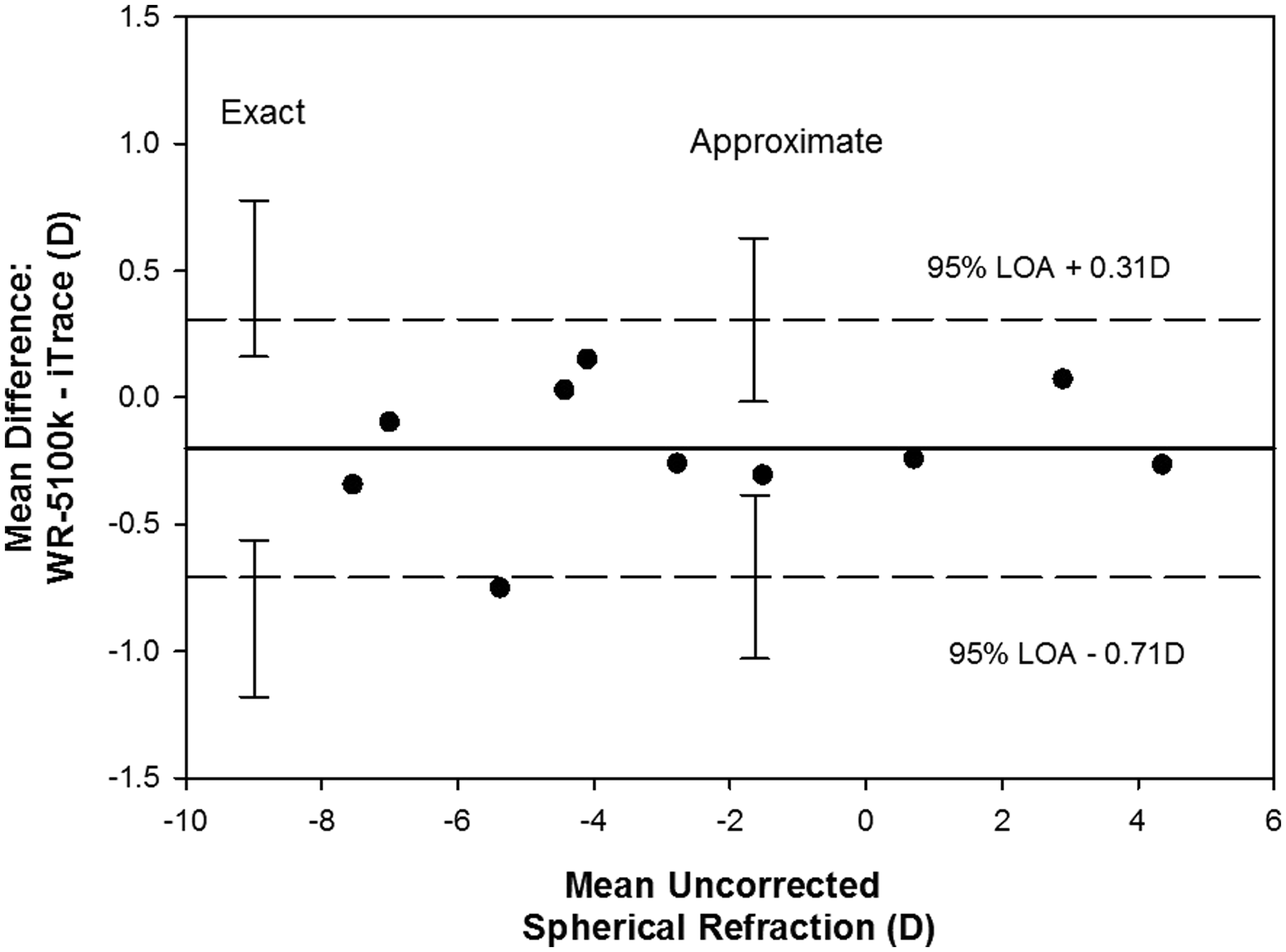
Figure 1 illustrates a Bland–Altman plot for method comparison data taken from a study of refractive error in eyes.¹² The data are from 10 participants (n = 10) and show measurements of spherical equivalent refraction in Dioptres (D) made using two automated instruments: WR 5100K and ITrace. A typical Bland–Altman analysis has the differences d between the two instruments (in this case WR 5100K-ITrace) plotted on the y-axis and the mean x_ave of the two measurements plotted on the x-axis. The mean of differences $\bar{d}$ (in this case −0.20 D) is shown as a horizontal reference line. The standard deviation of the differences, S_d, was 0.26 D.

Figure 1.

Bland–Altman plot comparing two methods of measuring ocular refractive error, data taken from 10 subjects.¹² Error bars represent 95% confidence limits for LOAs calculated using exact two-sided tolerance factors¹⁰ (asymmetric limits) and by Bland and Altman’s 1999 approximation (symmetrical limits).⁴

Bland–Altman analysis typically involves the calculation of upper and lower 95% LoA. Bland and Altman’s 1986 paper gave the LoA as

LoAs = \bar{d} \pm 2 S_{d}

(1)

Bland and Altman in 1986 acknowledged that the coefficient 2 was an approximation for 1.96, and most authors would use the slightly different definitions for LoA given by Bland and Altman (1999)⁴

LoAs = \bar{d} \pm 1.96 S_{d}

(2)

In Figure 1, equation (2) has been used to calculate the upper and lower LoAs. The upper LoA is −0.20 D +1.96×0.26 D = +0.31 D and the lower LoA is −0.20 D −1.96 × 0.26 D = −0.71 D.

The 95% LoAs are meant to represent the limits between which one would expect 95% of the inter-method differences to lie.^2,13 It is likely that many researchers think of 95% LoAs in this fashion, but it is actually a simplification. LoAs are calculated using sample statistics $\bar{d}$ and S_d: sample statistics which are only estimates of the population parameters. These sample statistics may have relatively large confidence intervals especially when sample sizes are small. Thus, there may be uncertainty about how well the LoAs calculated from the sample reflect the range over which 95% of the values would lie in the population.

This issue is important because researchers and readers will use LoAs to assess whether two techniques (or repeated measures) match well enough to give the same measurement from a functional point of view. Some authors argue that researchers using Bland–Altman analysis should explicitly establish acceptable bounds for LoAs before conducting the experiment.^14,15 But even if such a priori bounds are not established, readers are likely to interpret LoAs with their own, often unstated, opinions on what constitutes acceptable agreement. Such a judgement is difficult to make without an estimate of the potential uncertainty in LoA measurements.

As a means of addressing this issue, various authors have recommended calculating confidence intervals for LoAs.^{2,4,6,10,14–18} In this regard they are treating LoAs as most descriptive statistics should be treated (e.g. sample means, sample proportions, sample standard deviations).^15,19

This was discussed in one of the very early Bland and Altman papers² which described an approach whereby confidence intervals for LoAs (95% CL_LoA) are approximated by a t distribution

95 % {CL}_{LoA} ≅ {LoA \pm t}_{0.975, n - 1} \sqrt{3} \frac{s_{diff}}{\sqrt{n}}

(3)

Given Bland and Altman’s 1986 definition for LoAs (equations (1) and (2)) this could be rewritten as

95 % {CL}_{LoA} ≅ \bar{d} \pm 2 {S_{diff} \pm t}_{0.975, n - 1} \sqrt{3} \frac{s_{diff}}{\sqrt{n}}

(4)

Bland and Altman (1999) derived a slightly different coefficient for this approximation

95 % {{CL}_{LoA} ≅ LoA \pm t}_{0.975, n - 1} \sqrt{2.92} \frac{s_{diff}}{\sqrt{n}}

(5)

which, using their more precise definition for LoAs⁴ (equations (3) and (4)) could be rewritten as

95 % {CL}_{LoA} ≅ \bar{d} \pm 1.96 {S_{diff} \pm t}_{0.975, n - 1} \sqrt{2.92} \frac{s_{diff}}{\sqrt{n}}

(6)

Using equation (6), for the data in Figure 1, Bland and Altman’s approximate confidence limits would be −0.01 and +0.63 D for the upper LoA, and −0.39 and −1.03 D for the lower LoA. These approximate confidence intervals are shown in Figure 1. They lie symmetrically around the LoAs.

Bland and Altman (1999), in deriving this approximate method for LoA confidence limits, acknowledged that the approach assumes that n is not small. Likewise there have been other approximate methods for estimating LoA confidence limits^17,20 which also rely on the same assumption. This is unfortunate because it is for small samples that confidence intervals are likely to be the largest.

But there is an approach suggested by some authors^{6,9–11,21,22} which can work for any sample size, provided the inter-method differences can be assumed to be drawn from a normally distributed population. This approach to calculating confidence limits for LoAs involves using two-sided tolerance factors for a normal distribution. In the case of Bland–Altman analysis the problem can be expressed as: given a sample mean (for Bland–Altman analysis, $\bar{d}$ ) and a sample estimate of the standard deviation (for Bland–Altman analysis, S_d) what value of k fills the criterion that a minimum proportion, P (for 95% LoAs, P = 0.95) of the population lies between $\bar{d} \pm$ k S_d with confidence γ.²³ If one was interested in calculating a 95% confidence interval, then for the confidence limits that are closest to $\bar{d}$ , (the inner confidence limits), γ = 0.025 and for those confidence limits furthest from the mean (the outer confidence limits), γ = 0.975.

Ludbrook⁶ was the first to recommend this technique for outer confidence limits, using partial tables of two-sided tolerance factors derived from a very close approximation by Wald and Wolfowitz.⁷ Other authors have also used approximate two-sided tolerance intervals as descriptors of Bland–Altman LoAs.¹¹ Carkeet¹⁰ provided a more precise approach using an iterative method and the exact equations for two-sided tolerance factors^24,25

\frac{2 \sqrt{n}}{\sqrt{2 π}} \int_{0}^{\infty} P (γ, k | \bar{x}) e^{- 1 / 122 n {\bar{x}}^{2}} d \bar{x} = γ

(7)

where

P (γ, k | \bar{x}) = \Pr {χ^{2} > ν r^{2} / ν r^{2} k^{2} k^{2}}

(8)

and r is the root of the equation

P = \int_{\bar{x} - r}^{\bar{x} + r} φ (t) dt

(9)

and where φ(t) is the standard normal probability density function.

Carkeet¹⁰ provided tables of k values for γ values of 0.025, 0.05, 0.50, 0.95, 0.975. Although previous tolerance factor tables^8,24–26 have been published for γ values of 0.50, 0.95, 0.975, Carkeet’s tables¹⁰ for γ values of 0.025, 0.05 would appear to be unique in the literature, and they are necessary for calculating the inner confidence limits for LoAs.

By way of example, for the data in Figure 1 for n = 10 from Carkeet’s Table 2,¹⁰ for γ = 0.025, the k value for n = 10 (i.e. ν = n−1 = 9) is 1.3915.

So the inner confidence bounds for LoAs can be calculated as

{CL}_{LOA} = \bar{d} \pm {kS}_{d}

(10)

This would be −0.20 D + 1.3915 × 0.26 D = +0.16 D and −0.20 D − 1.3915 × 0.26 D = −0.56 D, and these bounds are shown in Figure 1.

Outer confidence limits can also be calculated from Carkeet’s Table 2,¹⁰ in which the appropriate k value for γ = 0.975 is 3.7706.

Using equation (10) the limits would be −0.20 D + 3.7706 × 0.26 D = +0.78 D and −0.20 D −3.7706 × 0.26 D =−1.18 D. These bounds are also shown in Figure 1.

To better compare the exact confidence limits found using two-sided tolerance factors with the Bland and Altman approximate confidence intervals, equations (4) and (6) and (10) can be used to calculate k values corresponding to Bland–Altman’s approximate confidence limits. For inner confidence limits they are

k_{approx} = 2 - t_{0.975, n - 1} \frac{\sqrt{3}}{\sqrt{n}} BlandandAltman (1986)^{2}

(11)

k_{approx} = 1.96 - t_{0.975, n - 1} \frac{\sqrt{2.92}}{\sqrt{n}} BlandandAltman (1999)^{4}

(12)

And for outer confidence limits

k_{approx} = 2 + t_{0.975, n - 1} \frac{\sqrt{3}}{\sqrt{n}} {BlandandAltman (1986)}^{2}

(13)

k_{approx} = 1.96 + t_{0.975, n - 1} \frac{\sqrt{2.92}}{\sqrt{n}} BlandandAltman (1999)^{4}

(14)

These values for k_approx can be compared with corresponding exact values of k to assess the closeness of Bland and Altman’s approximations. Alternatively, equations (7) to (9) can be used to calculate confidence values γ corresponding to Bland and Altman’s approximations from equations (11) to (14) (with P fixed at 0.95 for 95% LoA), and these confidence values can be compared with the ideal confidence values of 0.025 and 0.975, to assess the closeness of Bland and Altman’s approximation. As a further alternative, equations (7) to (9) can be used to calculate P values for Bland and Altman’s approximations from equations (11) to (14) (with γ fixed at the confidence values of 0.025 and 0.975), and P can be compared with 0.95 (for 95% LoAs), again to assess the closeness of Bland and Altman’s approximation. In the sections below, we adopt all three of these approaches to investigate Bland and Altman’s approximations. Our calculations were performed using MATLAB and iterative methods adjusting P or k until criterion gamma was calculated. P, k and γ were calculated to within eight decimal places, with the final precision being made finer by linear interpolation.

In addition, one can use two-sided tolerance intervals to evaluate Bland and Altman’s definitions of LoAs themselves. From Bland and Altman’s definitions 95% LoAs are $\bar{d} \pm$ 2S_d² and $\bar{d} \pm$ 1.96 S_d.⁴ Their reasoning for these limits was as follows:

‘If the differences are normally distributed, we would expect 95% of differences to lie between $\bar{d}$ − 1.96 S_d and $\bar{d}$ + 1.96 S_d (we can use the approximation $\bar{d} \pm$ 2 S_d with minimal loss of accuracy)’.⁴

This would only be true if the sample statistics $\bar{d}$ and S_d were equal to their respective population parameters μ_d and σ_d. This is true when sample sizes are infinite. For finite samples, $\bar{d}$ and S_d will have some uncertainty and one would expect LoAs to have uncertainty. Moreover, S_d is a biased estimate of σ_d, so one would expect $\bar{d} \pm$ 1.96 S_d to be biased estimates of the LoAs.

How large this bias is can be assessed using two-sided tolerance intervals. The problem might be considered by setting k = 1.96 (or k = 2) and asking the question: With what confidence, γ, can we state that at least that 95% (P) of the population lies between the limits $\bar{d} \pm$ k S_d? This can be calculated using equations (7) to (9). For small sample sizes this confidence is less than 50%, e.g. from equations (7) to (9), for n = 4 one can only state with a confidence of 0.314 (31.4%) that at least 95% of the population lies between $\bar{d} \pm$ 1.96 S_d (or the chance of at least 95% of the population not lying between $\bar{d} \pm$ 1.96 S_d is 68.6%).

Alternatively, one could use equations (7) to (9) to address the question, what value of k meets the criterion that at least 95% (P) of the population lies between the limits $\bar{d} \pm$ k S_d, with a confidence , γ, of 50%. That k value would give a ‘central’ estimate of LoAs in which there is a 50% probability that 95% of the population do not lie within these limits and a 50% probability that 95% of the population lie within these limits. In fact, such tables for k already exist^8,10 and show, for example, that when n = 4, one can state with confidence γ of 50%, that at least 95% of the population will lie between the limits of $\bar{d} \pm$ 2.4157 S_d (i.e. that k = 2.4157). These limits, for this small sample size, are considerably wider than k values of 1.96 or 2.

Yet another way of assessing this problem is (again using equations (7) to (9)) by setting k = 1.96 or (k = 2) and asking what proportion P of the population can be expected to lie between the limits $\bar{d} \pm$ k S_d with a confidence γ of 50%? For example, if n = 4, confidence γ = 0.50 and k = 1.96, then P = 0.886, i.e. an 88.6% LoA, not a 95% LoA.

All three of these measures are used below to evaluate the definitions of LoAs.

3 Calculations

3.1 Approximations for the outer confidence limits

Figure 2 shows, at different scales for clarity, how the k values for Bland and Altman’s approximate LoA outer confidence limits and the exact k values for two-sided tolerance factors (γ = 0.975) vary with sample size n, using equations (13) and (14). They also show k values calculated using exact two-sided tolerance factors based on equations (7) to (9). For low values of n the approximate method of Bland and Altman underestimate k, i.e. confidence limits actually lie further from $\bar{d}$ than would be indicated by Bland and Altman’s approximate limits. For the 1986 Bland and Altman approximation this occurs for sample sizes less than 40, and for the 1999, Bland and Altman approximation this occurs for sample sizes less than 76. For these smaller values of n the Bland and Altman approximate confidence limits will be too permissive, the difference being quite large for very small sample sizes. For n < 12 for the 1999 approximation and n < 11 for the 1986 approximation, this difference in k values will be greater than 0.5. For larger values of n (n >= 40 for the 1986 approximation and n >= 76 for the 1999 approximation), the Bland and Altman approximation will be slightly more conservative than the exact method, but will be a reasonable approximation, with k matching to within 0.02 for the 1999 approximation and to within 0.06 for the 1986 approximation.

Figure 2.

k values for outer LoA confidence limits calculated by exact two-sided tolerance limits (P = 0.95, γ = 0.975) (solid line) and corresponding to the 1986 approximation (equation (13)) (dashed line) and the 1999 approximation (equation (14)) (dotted line). A and B are the same curves presented at different scales to highlight different aspects of the data.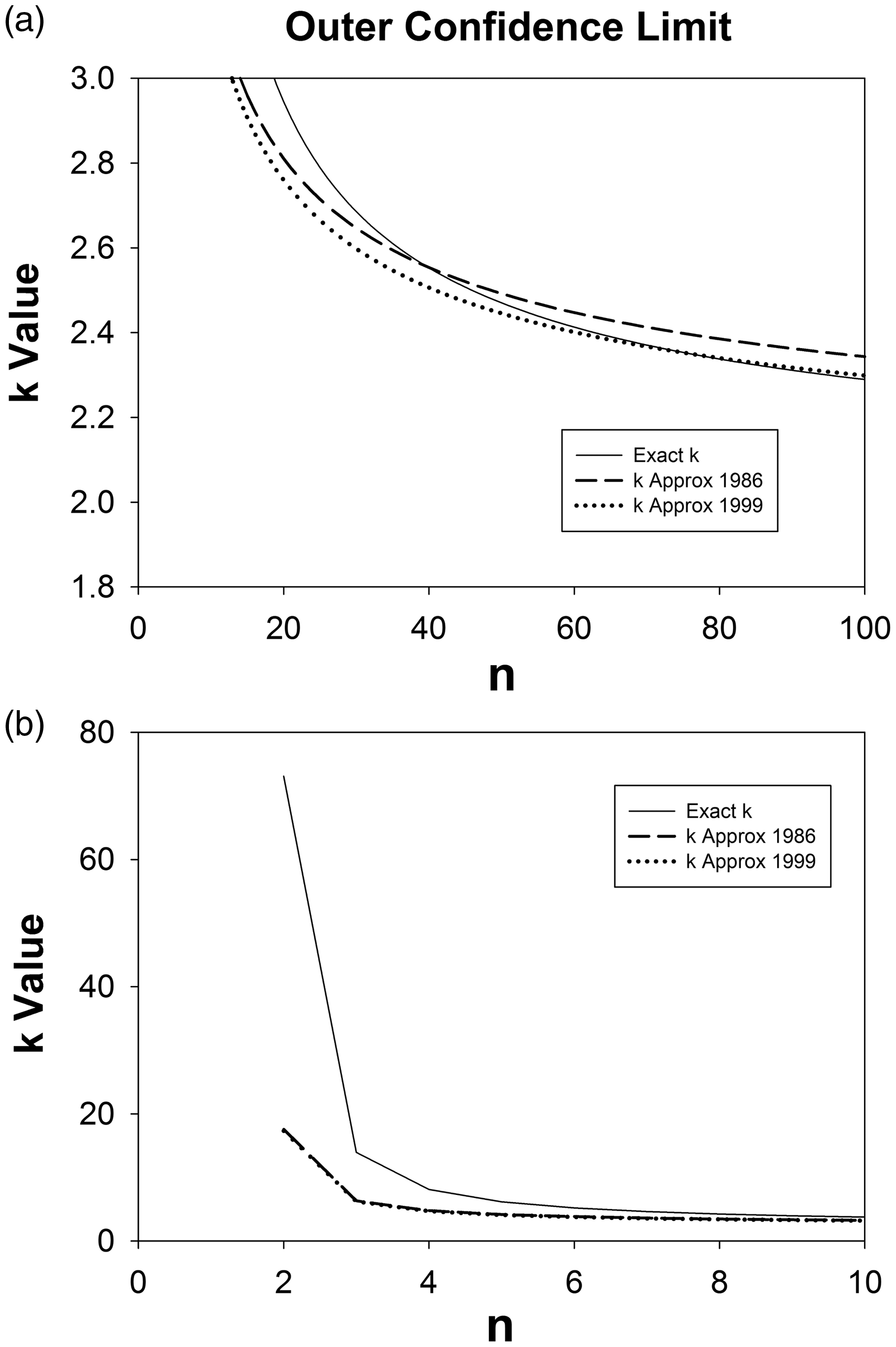

Using equations (9) to (11), it is possible to calculate actual confidence values for the 1986 and 1999 approximate outer confidence limits shown in Figure 2. This is shown at different scales in Figure 3, for different values of n. The actual confidence for these limits should be γ = 0.975. For low values of n the confidence limits are too permissive, but even for n = 2 the actual confidence limits described by Bland–Altman approximations are γ = 0.895 (1999 approximation), and γ = 0.896 (1986 approximation). The confidence limits will again become too conservative (i.e. > 0.975) when n >= 40 for the 1986 approximation and n >= 76 for the 1999 approximation and will approach γ = 1 as n approaches infinity.

Figure 3.

Confidence levels for the approximate outer confidence limit for 95% LoAs. The dotted line is for the 1986 approximation (k calculated using equation (13)) and the dashed line is for the 1999 approximation (k calculated using equation (14)). The solid line shows the goal confidence level of 0.975. A and B show the same curves to different scales.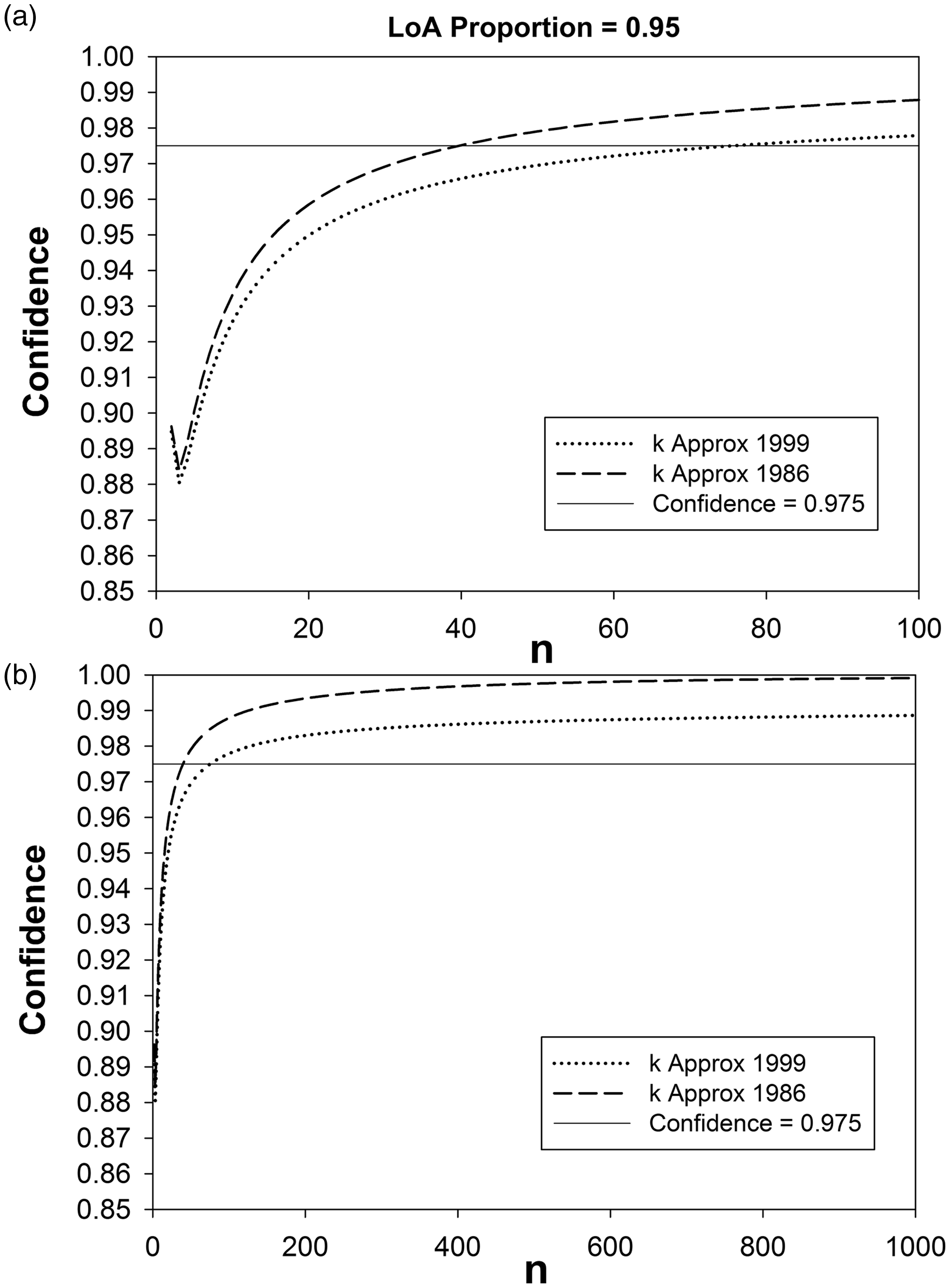

Finally, we have calculated what probability coverage for LoA would correspond to the Bland–Altman approximations for outer confidence limits if γ = 0.975. This can be done using equations (9) to (11). The results are shown at different scales in Figure 4. For n = 2, the Bland–Altman approximations for 97.5% confidence limits apply for 32.6% LoAs (1986 approximation) and 32.2% LoAs (1999 approximation) but approximate LoAs exceed 90% coverage at n = 10 with 90.7% LoAs (1986 approximation) and 90.1% LoAs (1999 approximation). For γ =0.975, LoAs will be conservative (covering greater than 95% of the population) for n >= 40 (1986 approximation) and n >= 76 (1999 approximation). Maximum probability coverage is 95.21% for the 1999 approximation (n = 306) decreasing to 95.0004% as n approaches infinity. For the 1986 approximation, maximum probability coverage is 95.63% for the 1986 approximation (n = 326) decreasing to 95.45% as n approaches infinity.

Figure 4.

LoA proportions covered for the outer (γ = 0.975) confidence limit for the 1986 approximation (dotted line) (k calculated using equation (13)) and for the 1999 approximation (dashed line) (k calculated using equation (14)). The solid line shows the goal LoA of 0.95 (i.e. 95% LoAs). A and B show the same curves to different scales.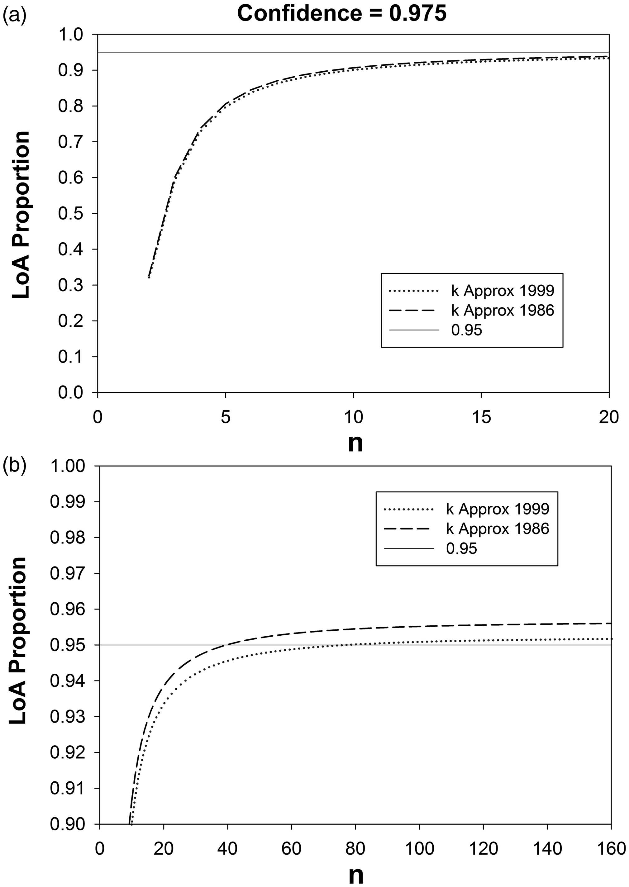

3.2 Discussion: Outer confidence limit approximations for LoAs

The Bland and Altman approximations for 95% LoA outer confidence limits are reasonable for larger values of n, becoming slightly conservative for values of n >= 40 for the 1986 approximation and n >= 76 for the 1999 approximation. For smaller values than this, the approximations will be permissive, but whether the approximation is reasonable will be a matter of judgement for researchers and readers. As a guideline if n >= 22 for the 1986 approximation and if n >= 27 for the 1986 approximation, then the Bland–Altman estimates of outer confidence limits for LoAs would be conservative for 94% LoAs, and this may be an acceptable approximation for researchers. For n values less than approximately 10, then the Bland and Altman approximations for outer confidence limits for LoAs will be poor, and exact methods of estimating confidence intervals for LoAs may be preferable.

3.3 Approximations for the inner confidence limits

Bland and Altman’s approximations for the inner confidence intervals (γ = 0.025) for 95% LoAs have some unusual properties. For low values of n (<= 5) the approximations for k can be negative, but exact two-sided tolerance factors can never be negative, by definition. This is shown in Figure 5.

Figure 5.

k values for inner LoA confidence limits calculated by exact two-sided tolerance limits (P = 0.95, γ = 0.0.25) (solid line) and for the 1986 approximation (equation (11)) (dashed line) and the 1999 approximation (equation (12)) (dotted line). A and B are the same curves presented at different scales.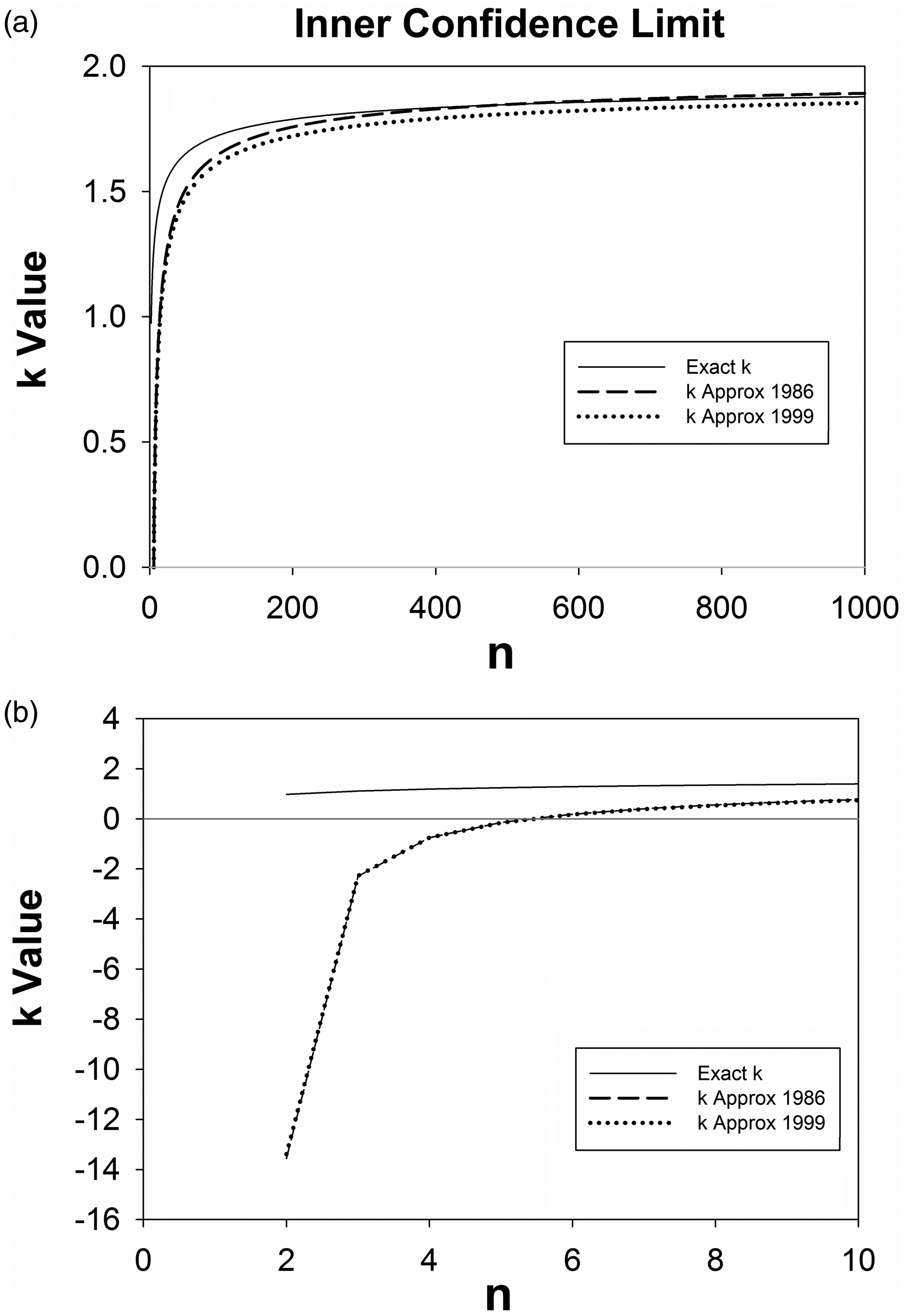

This would give the result that the approximate inner confidence limit for the upper LoA would lie below $\bar{d}$ and the inner confidence limit for the lower LoA would lie above $\bar{d}$ , and 95% confidence intervals for the upper and lower LoAs would overlap.

For sample sizes > 5, the approximate confidence limits will be too permissive (i.e. the confidence limits will be too close to $\bar{d}$ ) for all n values (except very extreme sample sizes) for the 1999 approximation and for the 1986 approximation for n values less than 489. For n values of 489 or greater the 1986 approximation gives k values that are slightly too conservative (by <=0.04).

Even at moderate values for n there is a reasonable difference between k values obtained by approximate methods and exact methods. For example, when n = 30 for a 95% LoA with γ = 0.025, the exact value for k is 1.508, but the equivalent values for the Bland and Altman approximations are 1.3532 (1986 approximation) and 1.3219 (1999 approximation).

The actual confidence values for Bland and Altman’s approximate inner confidence intervals for 95% LoAs are shown in Figure 6 for values of n up to 1000. For n values of 5 or less, the actual confidence is zero (i.e. such LoAs can never occur in the population, because k < 0). Over the range shown (n =<1000), the confidence level increases but is much too permissive, for the 1999 approximation (e.g. γ = 0.0051, for n = 1000), while for the 1986 approximation confidence increases more rapidly with n so that at n = 489, confidence becomes greater than 0.025. Both approximations (1986 and 1999) will have a confidence (γ) which will approach unity as sample size approaches infinity.

Figure 6.

Confidence levels for the approximate inner confidence limit for 95% LoAs. The dotted line is for the 1986 approximation (k calculated using equation (11)) and the dashed line is for the 1999 approximation (k calculated using equation (12)). The solid line shows the goal confidence level of 0.025. A and B show the same curves to different scales.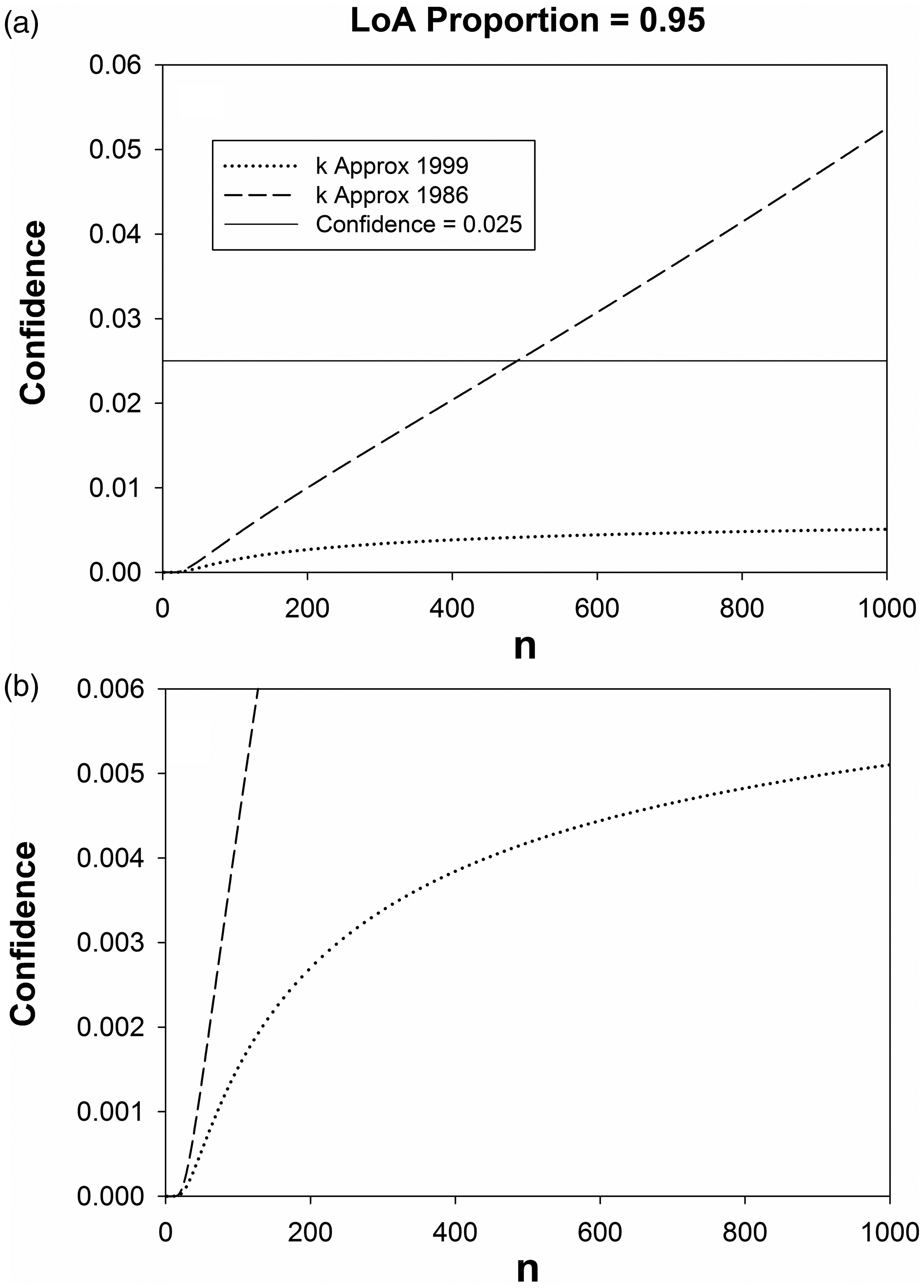

If one assesses the probability coverage for the LoA at γ = 0.025 for the Bland–Altman approximations (Figure 7), then for sample sizes <=5 coverage probabilities would have impossible values <0% (i.e. <0% LoAs) and are not plotted. At n = 6 for γ = 0.025 then the approximate inner confidence limits from Bland and Altman would correspond to 20% LoAs for the 1999 approximation and 21.9% LoAs for the 1986 approximations. For moderate sample sizes the coverage will still be too permissive, e.g. for n = 30 the Bland–Altman approximate inner bounds would correspond to γ = 0.025 for 89.9% LoAs (1999 approximation) and 90.7% LoAs (1986 approximation).

Figure 7.

LoA proportions covered for the inner (γ = 0.025) confidence limit for the 1986 approximation (dotted line) (k calculated using equation (11)) and for the 1999 approximation (dashed line) (k calculated using equation (12)). The solid line shows the goal LoA of 0.95 (i.e. 95% LoAs). A and B show the same curves at different scales.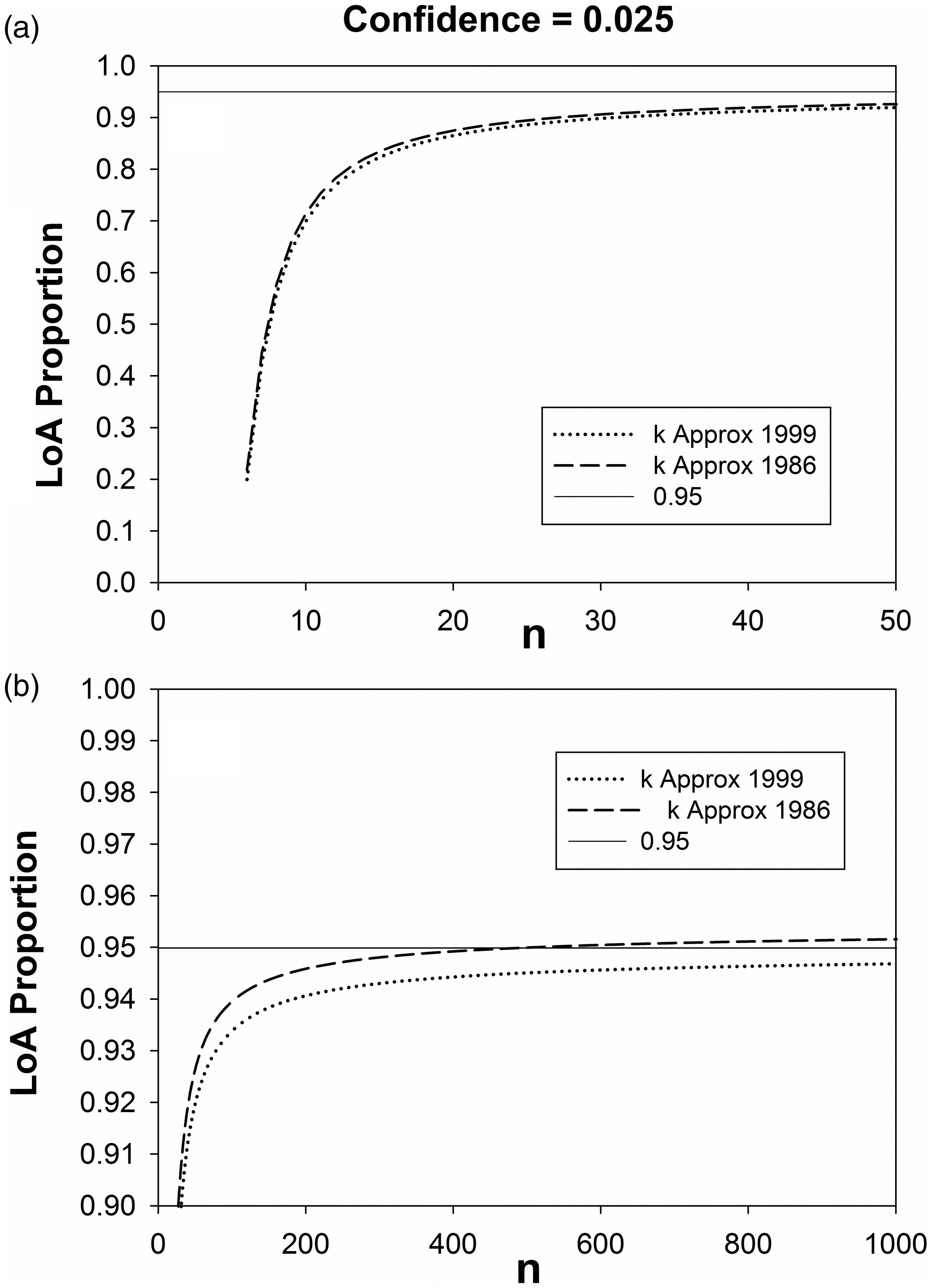

Eventually, as n increases, the approximate confidence limits for LoAs will become conservative (>95%) so that as n approaches infinity the Bland–Altman approximate inner bounds would correspond to γ = 0.025 for 95.0004% LoAs (1999 approximation) and 95.45% LoAs (1986 approximation).

3.4 Discussion: Inner confidence limit approximations for LoAs

Compared with outer confidence limits, Bland and Altman’s approximations for LoA inner confidence limits are a poorer approximation for the exact inner confidence limit based on two-sided tolerance intervals. This reflects the asymmetry of two-sided tolerance intervals, especially for low values of k. Its probability density function will be positively skewed with a long tail for high values of k. But low values of k are limited to values larger than zero, and this section of the probability density function is compressed. Bland and Altman’s approximations give negative k values for sample sizes <=5, which are difficult to find a meaningful interpretation for.

But even for larger sample sizes the approximations might not be adequate. As a guide, Bland and Altman’s inner confidence intervals would be appropriate (γ = 0.025) for 94% LoAs when n =>103 for the 1986 approximation and when n=>181 for the 1999 approximation. The 1986 Bland and Altman approximations for inner confidence intervals will be permissive for values of n < 490. For all practical sample sizes, the 1999 Bland and Altman approximation for inner confidence intervals will be too permissive, but for very large sample sizes (not shown in Figures 5 to 7) the 1999 approximation for inner confidence intervals will be conservative. This occurs because the 1.96 coefficient is not an exact approximation (slightly large) for the 97.5 percentile of the normal distribution. The exact transition sample size, where the 1999 approximation becomes conservative, is so large that it is difficult to calculate exactly with our software, but it is larger than 308,000,000 and smaller than 310,000,000.

Given that the Bland and Altman approximations for inner confidence intervals for 95% LoAs are permissive for sample sizes that are large in a practical sense, researchers may prefer the approach of using the exact two-sided tolerance factors to calculate the inner confidence limits.

3.4.1 LoA as estimates

Figure 8 shows k values (for P = 0.95 and γ = 0.50) for different sample sizes (Carkeet’s¹⁰ Table 2). For small sample sizes these k values are significantly larger than the LoA coefficients of 1.96 and 2 used in the Bland–Altman approximations.^2,4 By way of example for n = 2, the smallest sample size, k = 3.3756; while for n = 10, k = 2.1239. The k values decrease as n increases, becoming less than the Bland–Altman approximation of 2 for sample sizes greater than 40, and becoming less than the Bland–Altman approximation of 1.96 for sample sizes of greater than 45,349.

Figure 8.

k values for the median of the LoA confidence interval calculated by exact two-sided tolerance limits (P = 0.95, γ = 0.50) (solid line) and for the 1986 LoA (k = 2) (dashed line) and the 1999 LoA (k = 1.96) (dotted line).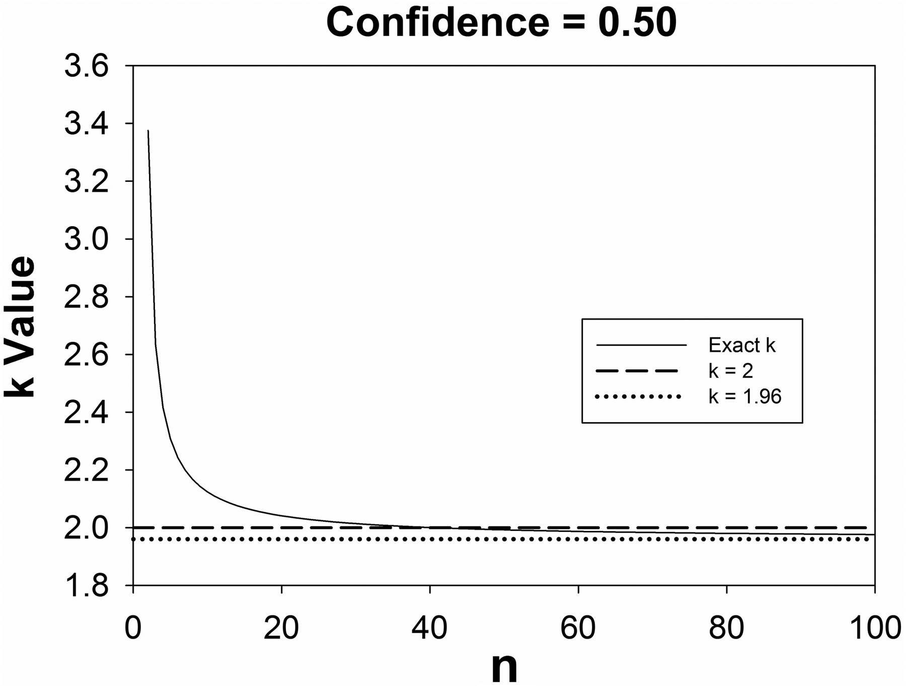

If k values are fixed at 2 or 1.96, and P = 0.95 (for 95% LoAs), then confidence levels γ can be calculated for different values of n, using equations (7) to (9). These γ values are shown, plotted against n, in Figure 9. For the k value of 2, confidence values are less than 0.50 for n values of less than 40, i.e. too permissive. But for the more commonly used approximation of k = 1.96 confidence values are too permissive for sample sizes that might not be considered small from a practical point of view. For example, confidence is less than 0.45 for n values less than 85; when n = 1000 confidence is 0.4855. For k = 1.96 confidence levels finally become greater than 0.5 when n > 45,349.

Figure 9.

Confidence levels for the Bland–Altman 95% LoAs. The dotted line is for the 1986 approximation (k = 2) and the dashed line is for the 1999 approximation (k = 1.96). The solid line shows the 0.5 confidence level. A and B show the same curves to different scales.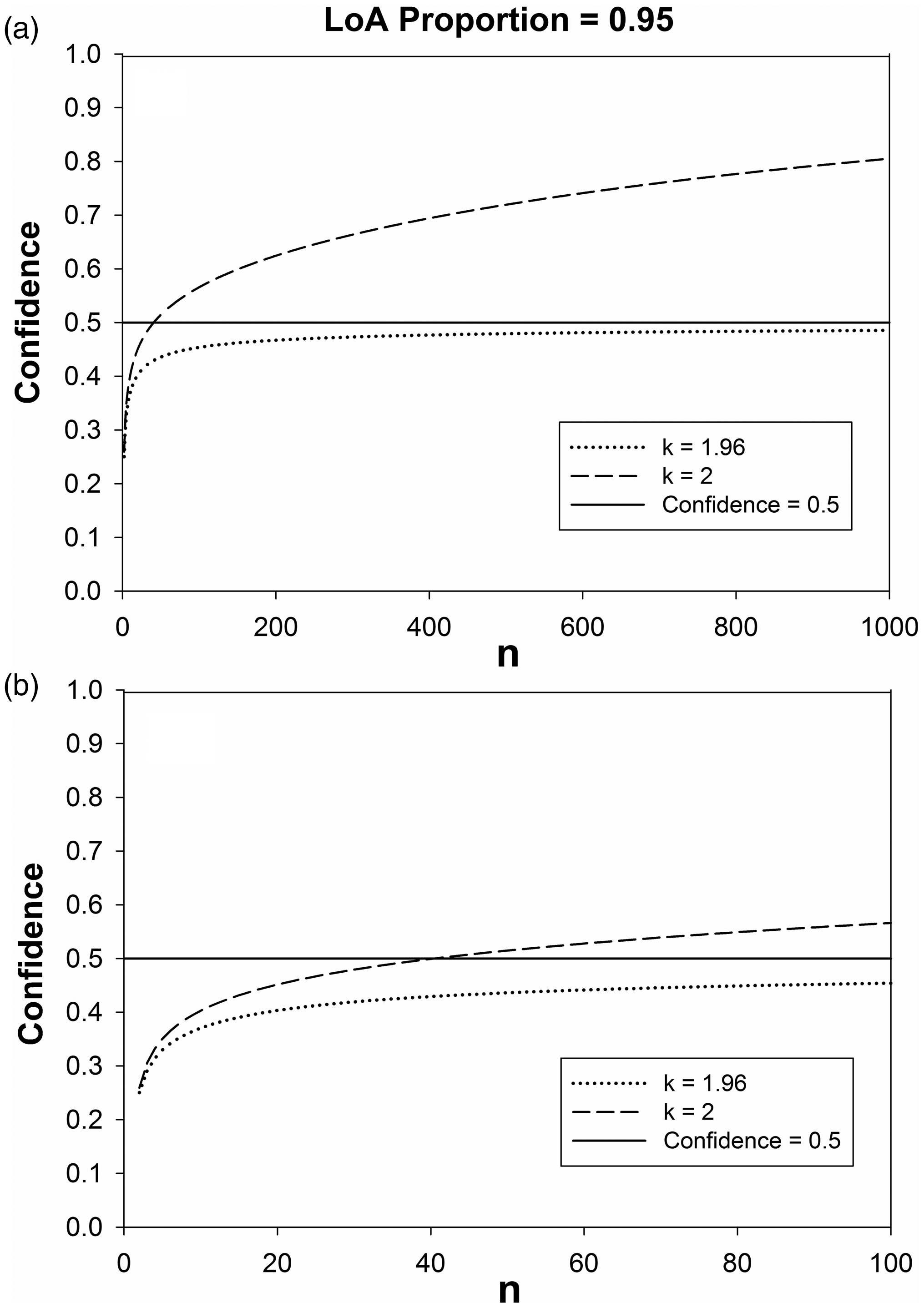

If, confidence levels are set at γ = 0.50, and k values are fixed at 2 or 1.96 then P values can be calculated for different values of n, using equations (7) to (9). These P values are shown, plotted against n, in Figure 10. Such P values are permissive for small sample sizes but P coverage may be acceptable for some researchers. For example for n = 2, P = 0.7358 (i.e. 73.58% LoAs) for k = 2 and P = 0.7255 (i.e. 72.55% LoAs) for k = 1.96. For n = 5, P becomes greater than 0.9 (e.g. wider than 90% LoAs) for k = 2 and for k = 1.96, and P becomes greater than 0.94 (i.e. wider than 94% LoAs) for n >= 14 for k = 2, and for n >= 20 for k = 1.96.

Figure 10.

LoA proportions covered for the median of the confidence interval (γ = 0.5) for the 1986 approximation (dotted line) (k = 2) and for the 1999 approximation (dashed line) (k = 1.96). The solid line shows the goal LoA of 0.95 (i.e. 95% LoAs). A and B show the same curves at different scales.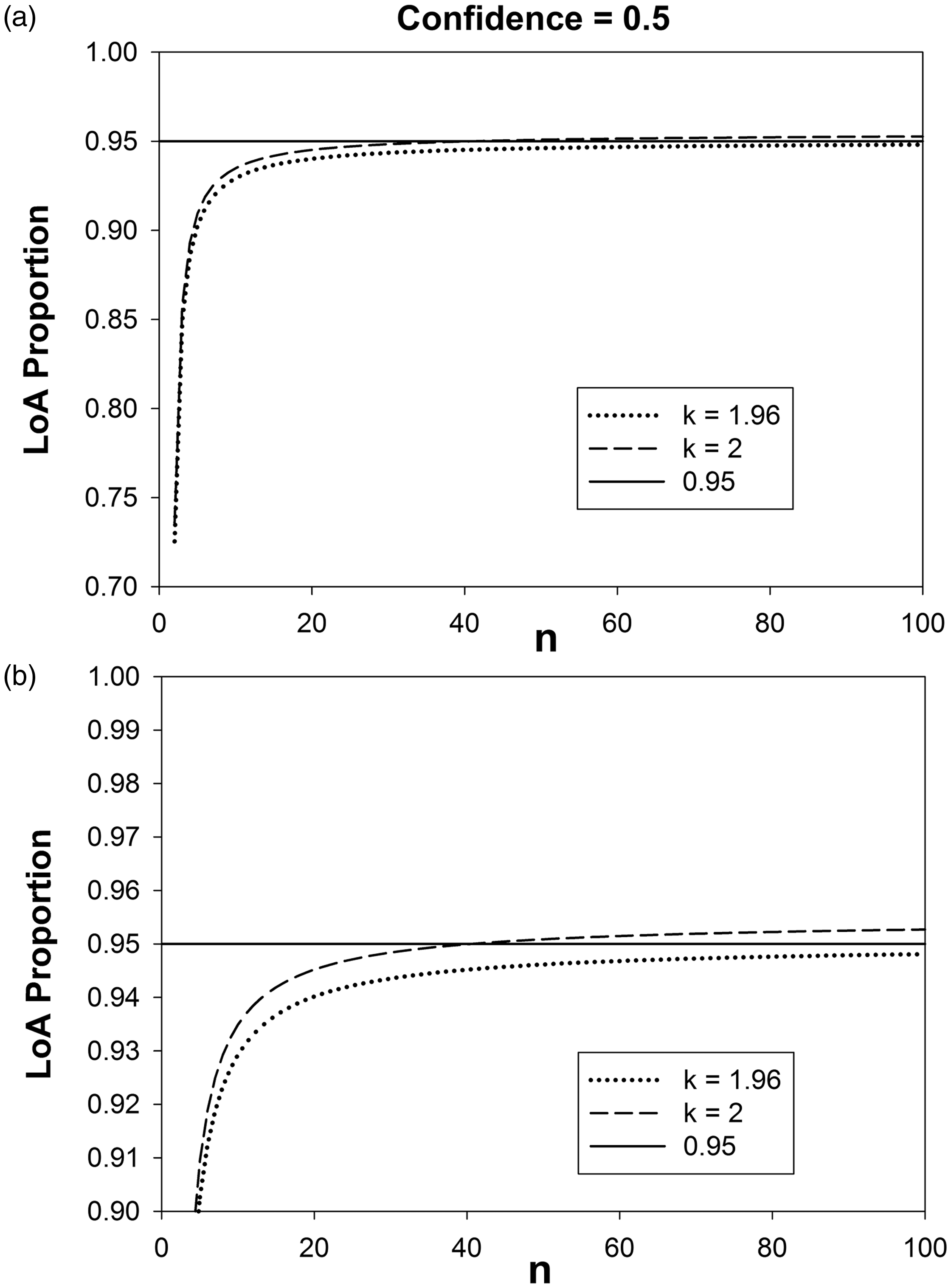

3.5 Discussion on LoA approximations

LoAs as defined by Bland and Altman cannot exactly summarize the possible range that contains 95% of the differences in the population. One can however describe a confidence interval for k values such that $\bar{d} \pm$ k S_d contains 95% of the population. We have chosen the 50th percentile in that confidence interval to give a k value which is representative of an LoA. If such a criterion is adopted we can say there is a 50% chance that at least 95% of the population will be contained within $\bar{d} \pm$ k S_d and a 50% chance that it will not. We think this is a reasonable approach, but we note that this median value is not the only possible measure of central tendency in the confidence interval. We could have, for example, adopted a mean value of the probability density function describing the confidence interval, but we note that, especially for small sample sizes, the probability density function is highly positively skewed (e.g. see Carkeet¹⁰ Figure 2) and such mean values have the potential to be very large. Moreover, their computation would require integration from zero to infinity, and thus the computational approach used in this paper cannot easily be applied.

Adopting a confidence of 50% as our criterion, Bland and Altman’s definitions of 95% LoAs as $\bar{d} \pm$ 2S_d and $\bar{d} \pm$ 1.96 S_d are reasonable approximations for many applications. The approximations would describe 94% LoAs when sample sizes are greater than or equal to 14 (for k = 2) and greater than or equal to 20 (for k = 1.96). This is likely to be an adequate approximation for most researchers, the difference being small compared with differences that might arise from other practical problems, e.g. possible violations of normality. For smaller sample sizes, it may be better to use the k values for two-sided tolerance factors with γ = 0.50. These will give slightly wider, more appropriately conservative bounds.

4 General discussion

The theoretical framework behind two-sided tolerance factors is well established and appears to be appropriate for considering Bland–Altman 95% LoAs. The basic data available are a sample mean $\bar{d}$ and a sample deviation S_d and it is possible to compute values of k that so that 95% of a population would be expected to lie between $\bar{d} \pm$ k S_d with a given confidence. This appears to nicely describe the underlying framework for LoAs and is a relatively practical approach.

Why then have approximate methods of describing confidence intervals for LoAs been predominantly used and described in the existing literature? One reason may be the availability of tables of two-sided tolerance factors. Approximate tables based on Wald and Wolfowitz method have been available since just after the Second World War^7,27 but it wasn’t until the early 1980s that extensive tables became widely available^8,26 based on exact computational methods.^24,25 It was not until 2015 that tables were published for two-sided tolerance factors for γ = 0.025 (and γ = 0.05)¹⁰ which are useful for determining inner confidence limits for LoAs. Thus, Bland and Altman were using the tools which were available to address the problem at that time.^2,4

A second issue may be one of the conceptual framework on which confidence intervals are based. Two-sided tolerance factors are used for addressing what portion of a population lies between $\bar{d} \pm$ k S_d with a given confidence. But previous methods of addressing the issue have adopted, either deliberately or unconsciously, an approach which estimates one-sided tolerance limits. One-sided tolerance factors address a slightly different issue. Expressed in Bland–Altman terms: one-sided tolerance factors assess the question: for a sample mean $\bar{d}$ and a sample standard deviation S_d what value of k₁ fills the criterion that a given proportion P (in this case 97.5%) of the population is less than $\bar{d}$ + k₁ S_d with a confidence γ. Such an approach is explicitly stated by Donner and Zou and by Zou as underlying their ‘MOVER’ approximation.^17,20 It is also likely to underlie (although not explicitly stated) Bland and Altman’s approximation approach⁴ to determining confidence intervals for LoAs, which gives Var( $\bar{d}$ ) + 1.96² Var(S_d) as the variance of the 95% LoAs: a step which approximates the variance in $\bar{d}$ + 1.96 S_d. We think the fundamental Bland–Altman question on LoAs is one that, based on the sample mean and a sample standard deviation, describes symmetrical limits on either side of the sample mean that contain 95% of the values in a population. This is a different problem from that addressed by one-sided tolerance factors. We note that if researchers have applications which are better addressed by one-sided tolerance factors, exact tables for these are also available¹⁰ and may be preferred to approximate confidence intervals.

A third issue may be that confidence intervals for LoAs are almost never reported in the literature. This is despite the fact that Bland and Altman first described how to calculate approximate confidence limits as early as 1986.² In a review of papers in one journal, such confidence limits had been reported in only 0.7% of papers using Bland–Altman analysis.¹⁰ Another literature review of laboratory research papers reporting Bland–Altman Analysis published later than 2012 found that 6% of these reported confidence intervals on their LoAs.¹⁵ Thus, researchers may not be used to thinking about LoA confidence intervals, exact or approximate, and there may be little incentive to develop different methods of calculating the confidence intervals.

Although it is not currently common practice, we think that reporting confidence intervals for LoAs should be a standard component of Bland–Altman analysis. It is important because the LoAs are used for comparison with clinical acceptable criteria for acceptance. It is good practice to establish such criteria and state them a priori, and a recent review found this done in 74% of papers assessed.¹⁵ But even if such criteria are not made explicit by authors, readers are likely to have their own reference criteria for acceptability. Researchers and readers should make this comparison with an understanding of the intrinsic uncertainty of LoAs, and confidence limits are a way of doing this. Providing such confidence intervals is considered good practice for many other statistics, such as sample means, odds ratios and risk ratios^5,19,28 and it is reasonable to treat LoAs in the same way. We note that other authors have also suggested that researchers should include a calculation of confidence limits for LoAs.^{2,6,14–16,18,29–31} These authors have usually recommended the approximate methods of Bland and Altman^2,4 (but not all⁶). Our results show that even for relatively large sample sizes the approximate method will not be sufficiently accurate.

This will be especially true for inner confidence limits, in which the approximation will give confidence limits on the wrong side of $\bar{d}$ for n <= 5 and will still give relatively permissive estimates for values of n = 30. It may be better that researchers use exact methods for calculating confidence limits for LoAs, especially for small sample sizes.

We note that, based on similar reasoning, one might also question the usual definition of LoAs as $\bar{d} \pm$ 2 S_d or $\bar{d} \pm$ 1.96 S_d, and replace the coefficient with the two-sided tolerance factor k for γ = 0.50. For small sample sizes (n< approximately 14–20) these definitions are clearly permissive, 95% LoAs are more likely than not to lie outside the bounds of $\bar{d} \pm$ 2 S_d or $\bar{d} \pm$ 1.96 S_d, although the approximation will be close enough for most practical purposes at larger sample sizes. However, researchers have been using the standard definitions for more than three decades,^1,2 and it is difficult to argue with the weight of tradition and more than 26,000 citations.³ Readers and researchers should be aware of the risk of bias for small sample sizes when defining LoAs as $\bar{d} \pm$ 2 S_d or d± 1.96 S_d and should consider augmenting the definition of LoAs with a calculation based on two-sided tolerance factors for γ = 0.50. Even if the standard definitions for LoAs are used, one way of indicating this bias is to include the exact confidence limits for LoAs which show the asymmetry of the confidence interval.

Finally, it is important to acknowledge that the calculation of Bland–Altman LoAs has an underlying assumption that data are drawn from a population with a normal distribution. This assumption also underlies the two-sided tolerance factors used above. If this assumption is incorrect for a data set then it is unlikely that 95% of a population will be contained between the LoAs (or described by the tolerance factors with a given confidence). Unfortunately, for small sample sizes it is difficult to assess those assumptions and so, like a lot of parametric statistics,⁵ the LoAs should be viewed with some caution. Unfortunately, non-parametric estimates of 95% LoAs require larger sample sizes to achieve a reasonable level of confidence.

This may be less of a problem for Bland–Altman analysis because it assesses differences between methods, which will tend to be distributed in approximately normal distributions.^2,4 However, researchers should be sensitive to theoretical issues in their data (e.g. sampling artefacts, or floor and ceiling effects) which may lead to the differences not being normally distributed. The robustness of Wald and Wolfowitz’s approximate two-sided tolerance limits⁷ has been assessed by Canavos and Koutrouvelis,³² using gamma and t-distributions as the parent populations for Monte Carlo studies. They found two-sided tolerance factors were robust for P values of 0.90 unless distributions are very skewed or kurtotic, but this robustness failed for P = 0.95 (the P values which would apply for 95% LoAs). Canavos and Koutrouvelis did not test robustness for confidence levels of γ = 0.025 and γ = 0.975, or γ = 0.50, and to be directly applicable to Bland–Altman LoAs it is worth doing a more complete robustness study using these confidence limits and the exact two-sided tolerance factors for P = 0.95.

5 Conclusions

If researchers are content that their data are normally distributed then Bland–Altman LoAs should be accompanied by confidence limits and in our view, especially for smaller samples, the more conservative exact two-sided tolerance factors should be used for their calculation, rather than Bland and Altman’s approximate method.

Footnotes

Acknowledgements

The first author thanks Kevin Hanley for his helpful instruction on the integration techniques used in computing values from equations (7) to ().

Declaration of conflicting interests

The author(s) declared no potential conflicts of interest with respect to the research, authorship, and/or publication of this article.

Funding

The author(s) received no financial support for the research, authorship, and/or publication of this article.

References

Altman

Bland

. Measurement in medicine: the analysis of method comparison studies. Statistician 1983; 32: 307–317.

Bland

Altman

. Statistical methods for assessing agreement between two methods of clinical measurement. Lancet 1986; 327: 307–310.

Web of Science 2016.

Bland

Altman

. Measuring agreement in method comparison studies. Stat Methods Med Res 1999; 8: 135–160.

Altman

Machin

Bryant

, et al. Statistics with confidence: confidence intervals and statistical guidelines, 2nd ed. London: Wiley, 2013.

Ludbrook

. Confidence in Altman–Bland plots: a critical review of the method of differences. Clin Exp Pharmacol Physiol 2010; 37: 143–149.

Wald

Wolfowitz

. Tolerance limits for a normal distribution. Ann Math Stat 1946; 17: 208–215.

ISO. 16269-6. Statistical interpretation of data—part 6: determination of statistical tolerance intervals, 2014.

Carkeet

. Comment on: statistical methods for conducting agreement (comparison of clinical tests) and precision (repeatability or reproducibility) studies in optometry and ophthalmology. Ophthal Physiol Opt 2015; 35: 345–346.

10.

Carkeet

. Exact parametric confidence intervals for Bland–Altman limits of agreement. Optom Vis Sci 2015; 92: e71–e80.

11.

Francq

Govaerts

. How to regress and predict in a Bland–Altman plot? Review and contribution based on tolerance intervals and correlated-errors-in-variables models. Stat Med 2016; 35: 2328–2358.

12.

Win-Hall

Glasser

. Objective accommodation measurements in pseudophakic subjects using an autorefractor and an aberrometer. J Cataract Refract Surg 2009; 35: 282–290.

13.

Armstrong

Davies

Dunne

MCM

, et al. Statistical guidelines for clinical studies of human vision. Ophthal Physiol Opt 2011; 31: 123–136.

14.

Mantha

Roizen

Fleisher

, et al. Comparing methods of clinical measurement: reporting standards for Bland and Altman analysis. Anesth Analg 2000; 90: 593–602.

15.

Chhapola

Kanwal

Brar

. Reporting standards for Bland–Altman agreement analysis in laboratory research: a cross-sectional survey of current practice. Ann Clin Biochem 2015; 52: 382–386.

16.

Hamilton

Stamey

. Using Bland–Altman to assess agreement between two medical devices – don’t forget the confidence intervals!. J Clin Monitor Comp 2007; 21: 331–333.

17.

Donner

Zou

. Closed-form confidence intervals for functions of the normal mean and standard deviation. Stat Methods Med Res 2010; 21: 347–359.

18.

McAlinden

Khadka

Pesudovs

. Statistical methods for conducting agreement (comparison of clinical tests) and precision (repeatability or reproducibility) studies in optometry and ophthalmology. Ophthal Physiol Opt 2011; 31: 330–338.

19.

Gardner

Altman

. Estimating with confidence. Br Med J 1988; 296: 1210–1211.

20.

Zou

. Confidence interval estimation for the Bland–Altman limits of agreement with multiple observations per individual. Stat Methods Med Res 2013; 22: 630–642.

21.

Downie

. Automated tear film surface quality breakup time as a novel clinical marker for tear hyperosmolarity in dry eye disease. Invest Ophthalmol Vis Sci 2015; 56: 7260–7268.

22.

Downie

Keller

Vingrys

. Assessing ocular bulbar redness: a comparison of methods. Ophthal Physiol Opt 2016; 36: 132–139.

23.

Owen

. Handbook of statistical tables, Reading, MA: Addison-Wesley, 1962.

24.

Odeh

. Tables of two-sided tolerance factors for a normal distribution. Commun Stat Simulat 1978; 7: 183–201.

25.

Eberhardt

Mee

Reeve

. Computing factors for exact two-sided tolerance limits for a normal distribution. Commun Stat Simulat 1989; 18: 397–413.

26.

Odeh

Owen

. Tables for normal tolerance limits, sampling plans, and screening, New York: Marcel Dekker, Inc, 1980.

27.

Bowker

Tolerance limits for normal distributions. In: Eisenhart

Hastay

Wallis

(eds). Selected techniques of statistical analysis for scientific and industrial research production and management engineering, New York: McGraw-Hill Book Company, 1947, pp. 97–110.

28.

Altman

Bland

. Confidence intervals illuminate absence of evidence. BMJ 2004; 328: 1016–1017.

29.

Giavarina

. Understanding Bland Altman analysis. Biochem Med (Zagreb) 2015; 25: 141–151.

30.

McAlinden

Khadka

Pesudovs

. Agreement studies: clarification. Ophthal Physiol Opt 2012; 32: 439–440.

31.

Stöckl

Rodriguez Cabaleiro

Van Uytfanghe

, et al. Interpreting method comparison studies by use of the Bland–Altman plot: reflecting the importance of sample size by incorporating confidence limits and predefined error limits in the graphic. Clin Chem 2004; 50: 2216–2218.

32.

Canavos

Koutrouvelis

. The robustness of two-sided tolerance limits for normal distributions. J Qual Technol 1984; 16: 144–149.