A Bayesian approach to the g-formula

Abstract

Epidemiologists often wish to estimate quantities that are easy to communicate and correspond to the results of realistic public health interventions. Methods from causal inference can answer these questions. We adopt the language of potential outcomes under Rubin’s original Bayesian framework and show that the parametric g-formula is easily amenable to a Bayesian approach. We show that the frequentist properties of the Bayesian g-formula suggest it improves the accuracy of estimates of causal effects in small samples or when data are sparse. We demonstrate an approach to estimate the effect of environmental tobacco smoke on body mass index among children aged 4–9 years who were enrolled in a longitudinal birth cohort in New York, USA. We provide an algorithm and supply SAS and Stan code that can be adopted to implement this computational approach more generally.

Keywords

Bayesian causal inference g-computation semiparametric

1 Introduction

Epidemiologists often wish to estimate quantities that are easy to communicate and correspond to the results of realistic public health interventions, such as changes to treatment guidelines or policy. Recent developments in the field of causal inference have shown that, under stated assumptions, observational data can be used to estimate such quantities.¹ Robins’ generalized computation algorithm formula (the g-formula) is one example of an approach from that field.² Using a parametric version of the g-formula, we can easily compare risks or rates of a health outcome in a population of interest under different exposure distributions.³

One assumption of the parametric g-formula is that we have accurately modeled the association between the outcome of interest and both the exposures of interest and potential confounders. For example, if the rate for a particular outcome varies in a linear–quadratic function with exposure, then our model could capture that by including both a linear and a quadratic term for exposure. This assumption can be approximately satisfied by modeling the association using flexible models that incorporate nonlinear functions and interaction terms. In particular settings, such as the study of complex exposure mixtures, complex longitudinal data, or small data sets, this may result in the model smoothing over strata in which we have little or no data, resulting in highly unstable estimates.

Numerous statistical approaches have arisen for stabilizing model estimates in such scenarios. Of note, Bayesian approaches have shown promise for dealing with sparsely identified models through the use of parameter prior distributions to stabilize estimates that would be highly variable in an unpenalized maximum likelihood procedure.^4,5 Further, even a set of default shrinkage priors can improve parameter estimation in multivariable regression models. For example in Stein’s paradox (see, for example, Efron and Morris’s description⁶), the maximum likelihood estimator of a set of regression parameters will always be inferior to a well-chosen shrinkage estimator whenever the number of parameters exceeds two. The parametric g-formula is computationally intensive and requires modeling a large joint parameter space that includes the outcome of interest, confounders, and possibly exposure. When exposure and confounders are time varying, the modeling requirements increase. When models are specified (approximately) correctly, the parametric g-formula is a powerful inferential tool with applications in many fields of knowledge generation such as public health, environmental health, and medicine. A significant drawback of the parametric g-formula in the frequentist construction is that it relies on inadmissible estimators (i.e. we can always find a better estimator⁷) of a large number of model parameters, the maximum likelihood estimates.

The primary objective of the current manuscript is to outline a foundational framework for Bayesian causal inference in epidemiologic studies that can be adapted for situations in which frequentist estimators may not be ideal. Such situations arise in cases of sparse data due to small sample size, when the number of parameters approaches sample size, when meaningful prior information is available, when covariates are highly correlated,⁴ or when accounting for measurement error.⁸ In particular, we focus on the case of small samples when the nuisance parameters of the parametric g-formula may be highly unstable, leading to poor finite-sample characteristics of the parameters of interest. We hypothesize that, in the vein of Stein’s paradox, a Bayesian approach with default shrinkage priors can result in estimates of marginal, population parameters that can improve on our predictions of the outcome of public health actions or interventions. This work extends current work in Bayesian, causal inference^9–13 by taking a more general approach to the Bayesian g-formula.

Our work also builds on non-Bayesian approaches to estimating parameters of the g-formula, such as those given by Taubman et al,¹⁴ Ahern et al.,¹⁵ Westreich et al.,¹⁶ and Keil et al.³ In particular, the algorithm given in Section 3 is a Bayesian analog of the algorithm given by Taubman et al.,¹⁴ whereby we estimate the distribution of potential outcomes under exposure using the empirical distribution of predicted outcomes under hypothetical interventions on exposures. We show, using simulations, that finite sample characteristics of the g-formula can be improved by adopting a Bayesian framework. Thus, provided that causal assumptions are met, our Bayesian approach may provide more accurate predictions of potential public health interventions than other approaches. For example, in a recent example of the non-Bayesian g-formula, Keil and Richardson¹⁷ estimated the potential impact of interventions on arsenic exposure in a cohort of copper smelters. In that example, the authors addressed the effects of airborne arsenic exposure on lung cancer and heart disease mortality. The latter effect estimate was estimated imprecisely, in part due to the highly variable baseline risk of heart disease mortality. Our approach could be applied directly to improve such an analysis by providing shrinkage priors or by leveraging the numerous studies done of nonairborne arsenic exposure and heart disease, which could, for example, provide a reasonable prior range for the estimate of association between arsenic and heart disease mortality. We also show here that the Bayesian Lasso is a viable approach to variance reduction. We are not aware of alternative approaches that can directly leverage prior information or shrinkage estimators while still providing impact estimates for hypothetical exposures. Such estimates are essential in deriving exposures standards in occupational and environmental settings, where precise estimates of risk are necessary to address the cost–benefit between exposure control measures and population health.

The novelty of this work is based on four points: (1) we derive a Bayesian g-formula approach in the potential outcomes framework, (2) we show that the Bayesian g-formula is possible using off-the-shelf MCMC software, (3) we provide an example showing that the approach is naturally “modular” and can be used to incorporate existing Bayesian solutions to problematic data, and (4) we demonstrate that the Bayesian g-formula has desirable frequentist properties under some choices of default shrinkage priors. This last point indicates that the Bayesian g-formula may have useful practical applications in scenarios when the frequentist g-formula may typically be used.

In Section 2, we define notation and demonstrate the Bayesian g-formula in time-fixed data, and we discuss some potential settings of interest. We outline an algorithm in Section 3 that can be used to develop software for this approach in a general Markov chain Monte Carlo estimation framework. This algorithm builds on non-Bayesian approaches to estimating parameters of the g-formula, such as those given by Taubman et al.,¹⁴ Ahern et al.,¹⁵ Westreich et al.,¹⁶ and Keil et al.³ In particular, we focus on the use of Bayesian methodology to improve on the finite sample performance of the g-formula.

In Section 4, we assess the ability to improve parameter estimation using default shrinkage priors by simulation. In Section 5, we demonstrate our approach using a longitudinal study of environmental tobacco smoke exposure and childhood body mass index (BMI) and extend our approach to nonnormal shrinkage priors using a version of the Bayesian least absolute shrinkage and selection operator (LASSO).¹⁸ We close in Section 6 with a discussion of the assumptions underlying our approach and speculate about future extensions. In Appendix 1, we derive our approach for both the time-fixed and longitudinal settings and we supply code in Section 8 to implement our approach for SAS and Stan programming languages.

2 The Bayesian g-formula

2.1 The parametric g-formula

To simplify our presentation, in this section we nest our example in the context of an observed set of time-fixed variables, $O = (Y, X, L)$ , where Y is some utility function, in our example a binary endpoint such as all-cause mortality, X is a binary exposure of interest, such as the level (high or low) of criteria air pollutants, $(CO, {NO}_{x}, O_{3}, {SO}_{2}, Pb)$ , and L is a vector of potential confounders such as residence in an urban (versus rural) setting and annual income (above or below $80,000, say). A more general setting is given in Appendix 1.

In this setting, we are interested in the marginal distribution of the potential outcome $Y^{g} \in {0, 1}$ , where g refers to some intervention value (or distribution) for the exposures of interest. For example, we may be interested in the risk (i.e. cumulative incidence) of lung cancer in the population in which g represents low concentrations of the pollutants. In other words, our intervention is to “set” each of the pollutants to “low.” We assume that this hypothetical scenario corresponds to a well-defined intervention or set of interventions to reduce the pollutants to our specified level, such as mandating manufacturing changes to decrease vehicle exhaust emissions or restricting traffic on certain days. The risk under this intervention is given as $Pr (Y^{g} = 1)$ .¹⁹ For example, for binary L the g-formula estimate of the risk under intervention can be expressed using the law of total probability as

Pr (Y^{g} = 1) = \sum_{ℓ \in {0, 1}} Pr (Y^{g} = 1, L = ℓ) = \sum_{ℓ \in {0, 1}} Pr (Y^{g} = 1 | L = ℓ) Pr (L = ℓ)

To facilitate the expression of these quantities in a Bayesian framework, we adopt a more general notation and instead express the distribution of the potential outcome as

p (y^{g}) = \int_{ℓ} p (y^{g} | ℓ) p (ℓ) d ℓ

(1)

where the summation symbol has been replaced by an integral, and the discrete probability notation has been replaced by the generic probability function p. For a random variable A, if A is discrete then we let p(a) denote

Pr (A = a)

, the mass of A at realization a. Likewise, if A is continuous then we let p(a) denote f(a), the density of A at realization a. We also let

p (\cdot | a)

denote

p (\cdot | A = a)

. To simplify notation we allow that the integral expression

\int g (a) da

for a function g(a) of a will be used to denote integration if A is continuous under Lebesgue measure, i.e.

\int g (a) da

, and summation if A is discrete under counting measure, i.e.

\sum_{{a}} g (a)

. The formula given in equation (1) yields the population distribution of the outcome under the intervention g, where the “population” referred to here is the set of individuals with the distribution of L given by

p (ℓ)

The parametric g-formula extends the g-formula given in equation (1) by characterizing the conditional components $p (y^{g} | ℓ)$ and $p (ℓ)$ using parametric models. Thus, the parametric g-formula representation of the potential outcome distribution under intervention g is given as

p (y^{g}; β, η) = \int_{ℓ} p (y^{g} | ℓ; β) p (ℓ; η) d ℓ = \int_{ℓ} p (y | g, ℓ; β) p (ℓ; η) d ℓ

(2)

where the parameter vector β corresponds to the conditional change in the probability of Y for unit changes in X and L, and η corresponds to the parameters of the probability of L. The rightmost side of equation (2) is derived under counterfactual consistency²⁰ and relies on the assumptions of positivity, conditional exchangeability, and correct specification of models. Summary effect measures, such as the causal risk difference for a unit increase in X can be estimated using Monte Carlo methods.³

The utility of the g-formula becomes apparent when one considers that the functional form of the relationship between X and Y may be a complicated nonlinear function in nonbinary data, possibly with high-order interaction terms. Note that, under such a scenario, the counterfactual distribution $p ({\tilde{y}}^{g})$ is easily interpreted as the outcome distribution we would expect if we could have intervened to set X to g. Similarly, if L is high dimensional or X (and possibly L) is time varying, simple interpretations are still possible and can correspond to realistic settings. Thus, the approach provides results that are easy to communicate to nonspecialist stakeholders and have immediate public health utility. As a further consideration, the g-formula can be used to estimate unbiased net effects of exposure when X and L may affect each other over time, whereas regression model estimates will generally be biased for such parameters.²¹

The parameters β or η may not be stably estimated when L or X is of high dimension relative to the sample size, when estimating effects in small samples, or when there is high correlation between elements of the data (i.e. due to variance inflation or finite sample bias). In such settings, common approaches are to create a more parsimonious model, apply some penalization term/regularizing, or adopt a Bayesian framework to stabilize estimates using prior knowledge. We adopt an approach that recasts the parametric g-formula within a Bayesian framework as a way to embrace the interpretability of the g-formula approach while employing the variance reduction properties of Bayesian inference. We focus on shrinkage estimation, in which we allow the possible introduction of some bias in exchange for higher precision and an overall reduction in mean-squared error (MSE).

2.2 A Bayesian approach

Following Rubin²² and Saarela et al.,¹² we consider a Bayesian version of the potential outcome distribution, the posterior predictive distribution $p ({\tilde{y}}^{g} | o)$ . The posterior predictive distribution of the potential outcomes given by the Bayesian approach differs from the estimated distribution of potential outcomes using the standard g-formula in that it marginalizes over the posterior distributions of the parameters (β and η).

Our quantity of interest is the posterior predictive distribution of the potential outcome under the intervention g, which is defined as $p ({\tilde{y}}^{g} | o) \equiv \int p ({\tilde{y}}^{g} | θ) p (θ | o) d θ$ , where $p (θ | o)$ is the posterior distribution of the parameters θ (which describe the models of the relationships between Y, X, and L).

The posterior predictive distribution of the potential outcome under intervention g is given in our example as

p ({\tilde{y}}^{g} | o) = \int_{\tilde{ℓ}} p (\tilde{y} | g, \tilde{ℓ}, o) p (\tilde{ℓ} | o) d \tilde{ℓ} = \int_{\tilde{ℓ}} \int_{θ} p (\tilde{y} | g, \tilde{ℓ}, θ) p (\tilde{ℓ} | θ) p (θ | o) d θ d \tilde{ℓ}

Under counterfactual consistency and the assumptions of conditional exchangeability, positivity, and parameter variation independence (detailed in Appendix 1), $p ({\tilde{y}}^{g} | o)$ is a function only of the observed data, the target population distribution of L, the intervention value set by the analyst, and prior parameter distributions. We make these assumptions for the remainder of this section.

p ({\tilde{y}}^{g} | o) \propto \int_{\tilde{ℓ}} \int_{η} \int_{β} p (\tilde{y} | g, \tilde{ℓ}, β) p (\tilde{ℓ} | η) L (β | y, x, ℓ) L (η | ℓ) π (β) π (η) d β d η d \tilde{ℓ}

(3)

To conceptualize the computation, ${\tilde{Y}}^{g}$ acts like a missing variable that can be imputed after setting exposure to some value g.²³ In general, equation (3) and its extension to longitudinal data given in Appendix 1 will not be given in closed form, which necessitates MCMC approaches. MCMC software that can accommodate imputation of missing data may be used for the Bayesian g-formula.

3 Bayesian g-formula algorithm

Here we present an algorithm for estimation using the Bayesian g-formula to numerically approximate equation (3), as well as quantities derived from a comparison of ${\tilde{Y}}^{g}$ under two interventions, such as the 30-year risk difference comparing the study population under two different exposures, one version of the average causal effect. To generalize the outline given in Section 2 to longitudinal settings, we describe an algorithm for estimating parameters of the Bayesian g-formula when exposure and covariates may be time varying (the Bayesian g-formula in the time-fixed setting is just a special case of this longitudinal approach). For simplicity, we limit this approach to static, deterministic interventions such as “always treat” or “never treat.”

Generalizing our approach to the longitudinal setting requires choosing some time scale, such as time on study, calendar time, or age, and we denote specific points on that time scale as t, which we assume to be fine, yet discrete. We denote the value of the exposure at time t as X(t) and let the history of exposure up to and including time t be $\bar{X} (t) \equiv (X (0), \dots, X (t))$ . Time-varying covariate vectors $\bar{L} (t)$ and outcomes $\bar{Y} (t)$ are denoted similarly. In our notation $\bar{X} (t), \bar{L} (t)$ , and $\bar{Y} (t)$ are multivariate vectors with elements at times $0, \dots, t$ . In practice, these usually correspond to functional summaries over time that include only relevant aspects, such as the cumulative exposure through time t. The vector $(L (0), X (0), Y (0))$ contains the values of the covariates, exposure, and outcome we observe at the origin of the time scale of interest. Generally, L(0) includes time-fixed quantities such as race, sex at birth, or income at baseline.

We let ${\tilde{Y}}^{g} (t)$ and $\tilde{L} (t, g)$ represent values of the posterior predictive distributions of the potential outcome $Y^{g} (t)$ and the covariate vector L(t) under intervention g. These variable vectors are denoted in different ways to emphasize that we may be able to estimate the posterior distribution of the potential outcomes (a causal interpretation) under intervention g without making the additional assumptions necessary to estimate the distribution of the other postexposure covariates. We assume that L(t) occurs temporally before X(t), which both occur before Y(t), implying that $\tilde{L} (0, g) = \tilde{L} (0)$ . This allows us to nonparametrically sample $\tilde{L} (0)$ from the population empirical distribution $p_{N} (l (0))$ . Because we let $p_{N} (l (0)) = p (l (0) | η)$ and we let $\tilde{ℓ} (0) = ℓ (0)$ , our algorithm is more accurately described to estimate parameters of a semi-Bayesian, semiparametric g-formula.

After we have selected an appropriate target population (defined by $p (\tilde{ℓ} (0))$ and intervention of interest (defined by g), the Bayesian g-formula algorithm can be summarized in the following steps:

Specify the model for the joint likelihood Specify a joint model in the source population for ${L (t), X (t), Y (t)}$ . For static regimes, this corresponds to the following:

Specify a model for each component of $L (t)$ . One could conceivably fit a separate model at each t, which, for multivariate $L \equiv (L_{1}, \dots, L_{p})$ and $t = (0, \dots, K)$ equals p × K models. In practice, the elements L(t) are modeled using time-averaged (pooled) models that average coefficient values across time. If $L (t)$ consists of a single dichotomous variable this could be given as

logit {L (t) = 1 | \bar{x} (t - 1), \bar{l} (t - 1), \bar{Y} (t - 1) = \bar{0}; η} = η_{0} + η_{1} t + η_{2} \sum_{j = 0}^{t - 1} x (j) + η_{3} \sum_{j = 0}^{t - 1} ℓ (j)

Specify a time-averaged model (or set of time-specific models) for $Y (t) .$ Assuming that Y(t) is an indicator of death by time t, this model could be

logit {Y_{1} (t) = 1 | \bar{x} (t), \bar{l} (t), \bar{Y} (t - 1) = \bar{0}; β} = β_{0} + β_{1} t + β_{2} \sum_{j = 0}^{t} x (j) + β_{3} \sum_{j = 0}^{t} ℓ (j)

Both of these relatively simple models should be considered for illustrative purposes only because they are likely oversimplifications for realistic settings.

Specify the prior distributions For a static intervention, we need only define prior distributions $π (β)$ and $π (η)$ because modeling exposure is unnecessary. In most scenarios, investigators may be able to derive meaningful and relatively precise prior information for β because this model often corresponds to regression models used in the literature. Parameters for η may be more challenging because covariate model parameters are rarely reported. In many scenarios, the analyst will be unable to specify informative, nonnull distributions for some (or possibly all) parameters. One may, instead, specify reasonable generic information, such that the conditional log-odds ratios are likely to be within some interval. In epidemiologic practice, it is rare to see (for example) odds ratios outside of the range 1/10 to 10.²⁴ Therefore, weakly informative default priors result in shrinkage estimators that may improve predictive accuracy, which is a common justification for using Bayesian inference.²⁵

Sample from the target population Define and sample from a target population defined by $p (\tilde{L} (0))$ . This is often identical to the population by the observed sample, and the L(0) can be sampled by taking the empirical distribution of the baseline covariates in the data. The target population will be considered to be under observation for some fixed time k, such that $t \equiv {1, . ., k}$ .

Set the intervention values Define a static intervention $\bar{g} (m)$ such as “always exposed,” e.g. $g (t) = g = 1$ for all t. Set the exposures at all time points to this static intervention, i.e. $\tilde{X} (t) = g$ for all t. A parameter of interest could be the posterior predictive causal risk difference comparing “always exposed” to “never exposed.”

Draw from the posterior parameter distribution From our simple models in step 1, draws from the posterior distribution of the model parameters given in step 1 ( ${\hat{η}}_{0}, \dots, {\hat{η}}_{3}, {\hat{β}}_{0}, \dots, {\hat{β}}_{3}$ ) are interpreted as posterior, conditional log-odds ratios. These quantities are not of particular interest for our purposes but are used in the next step to generate posterior predictive values. This is the point where typical epidemiologic Bayesian analyses stop, because the posterior log-odds ratio is the parameter of interest in many settings.

Draw from the posterior predictive distribution Draw new values of $\tilde{L} (t)$ and $\tilde{Y} (t)$ in the target population by iteratively sampling values from the models in step 1 under intervention g(t). In our example, one could impute values of ${\tilde{L}}_{i} (1)$ by simulating random values from a Bernoulli distribution with a mean equal to ${logit}^{- 1} ({\hat{η}}_{0} + {\hat{η}}_{1} t + {\hat{η}}_{2} g + {\hat{η}}_{3} ℓ (0))$ . Similarly, $\tilde{Y} (1)$ would be imputed as a draw from a Bernoulli distribution with a mean of ${logit}^{- 1} ({\hat{β}}_{0} + {\hat{β}}_{1} t + {\hat{β}}_{2} g + {\hat{β}}_{3} (\tilde{ℓ} (1, g) + ℓ (0)))$ . One would then similarly draw values of $\tilde{L} (2)$ using ${logit}^{- 1} ({\hat{η}}_{0} + {\hat{η}}_{1} t + 2 {\hat{η}}_{2} g + {\hat{η}}_{3} (ℓ (0) + \tilde{ℓ} (1))$ among those with $\tilde{y} (1) = 0 .$ This process of sampling from conditional posterior distributions would continue iteratively for times $t = 2, \dots, k$ . Note that the posterior distributions of $\tilde{L} (t)$ and $\tilde{Y} (t)$ depend on the histories of the posterior draws up to time t

Estimate the parameter of interest For the survival outcome Y(t), we are interested in causal contrasts of the posterior potential outcome distribution $p (\bar{\sim} y^{g} | o)$ . For example, we can estimate the posterior potential risk difference at the end of follow-up, time m, defined as: ${rd}^{(1, 0)} (m) \equiv E ({\tilde{Y}}^{1} (m)) - E ({\tilde{Y}}^{0} (m))$ , by taking the difference of the sample posterior means of the imputed ${\tilde{Y}}_{i}^{g} (m)$ values

{\hat{rd}}^{(1, 0)} (m) = n^{- 1} (\sum_{i = 1}^{N} {\tilde{Y}}_{i}^{1} (m) - \sum_{i = 1}^{N} {\tilde{Y}}_{i}^{0} (k)) = n^{- 1} \sum_{i = 1}^{n} ({\tilde{Y}}_{i}^{1} (m) - {\tilde{Y}}_{i}^{0} (m))

The 95% posterior intervals could then be calculated by taking the 2.5th and 97.5th percentile of the posterior distribution of the risk difference or using an approximation such as taking ±1.96 times the standard deviation of the posterior distribution (a plug-in estimator of the standard error). This step could be modified by considering only the expected values of

{L (t, g), Y^{g} (t)}

at each time rather than simulating discrete values, as in Taubman et al.’s¹⁴ notable application of the frequentist g-formula.

4 Simulation study

We examine the impact of null-shrinkage priors in a Bayesian g-formula approach using two simple simulation studies in scenarios in which shrinkage parameters might typically be used. Our first simulation is in a time-fixed setting in which we have measured an exposure and a confounder that are highly correlated. Such settings are common in environmental epidemiology, such as in the air pollution literature where the effects of one pollutant might be difficult to estimate precisely due to high correlation with another pollutant from a similar source. Our second simulation deals with a simple, time-varying data scenario in small samples.

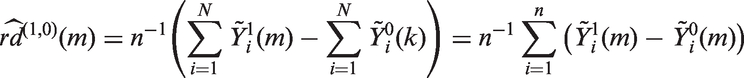
For both simulations, we are primarily interested in ${rd}^{(\bar{1}, \bar{0})}$ , the causal risk difference comparing “always exposed” and “never exposed” (referent). Thus, the hypothetical intervention g corresponds to exposing everyone or completely preventing exposure in a way that has no side effects (i.e. we assume the intervention is an instrument for exposure, much in the way that randomization is an instrument for treatment in a randomized clinical trial). The target population in both scenarios is the population implied by the observed sample. We estimate ${\hat{rd}}^{(\bar{1}, \bar{0})}$ using both the frequentist g-formula (“standard g-formula”) and the Bayesian g-formula. We calculate bias as ${rd}^{(\bar{1}, \bar{0})} - {\hat{rd}}^{(\bar{1}, \bar{0})}$ . For each simulation, we perform the analyses on M = 1000 simulated datasets and average the bias and MSE over samples.

For the standard g-formula, the risk difference and its standard error were estimated using a nonparametric bootstrap. For each of the M iterations, we created S = 1000 bootstrap samples of each of the M simulated datasets and calculated a risk difference using the Monte Carlo approach we described previously,³ which involves taking D draws from each bootstrap sample, where we set D = 2000. The risk difference for each of the M iterations was taken to be the mean risk difference across the S samples, and the standard error was calculated as the sample standard deviation for these S samples. Thus, for each analysis, the standard g-formula required simulation across $S \times M \times D = 2, 000, 000, 000$ units.

For the Bayesian g-formula, we analyzed each dataset using the MCMC procedure of SAS 9.4. Each analysis was performed using C = 10,000 iterations after a burn-in of B = 1000 iterations. We estimated ${\hat{rd}}^{(\bar{1}, \bar{0})}$ using the sample mean of the risk difference across all MCMC iterations, and we estimated the standard error of ${\hat{rd}}^{(\bar{1}, \bar{0})}$ by taking the sample standard deviation of the posterior draws of the risk difference. For each analysis using the Bayesian g-formula, we made $(C + B) \times M = 11, 000, 000$ posterior draws.

We calculated 95% confidence/credible intervals for each analysis by as the 2.5th and 97.5th percentiles of the bootstrap/MCMC estimates. Confidence/credible interval coverage was calculated as the proportion of all datasets for which the 95% confidence/credible intervals contained the true risk difference. We also compared the standard deviation of the bias across the M samples for each approach as a measure of precision. MSE, our primary metric of comparison, was calculated as the average across the M iterations of the squared bias plus the variance. We also calculated the mean-squared (in-sample) prediction error (MSPE) as the mean of the squared difference between individual predictions of ${rd}^{(\bar{1}, \bar{0})}$ and the true value. For most analyses MSE≈MSPE, so we only report MSE. We compared the MSE between the Bayesian g-formula and the standard g-formula using the ratio of the MSE for the Bayesian g-formula and the MSE for the standard g-formula. A value of the MSE ratio below 1 indicates that the Bayesian g-formula performs better than the standard g-formula in a bias–variance trade-off (with MSE as the loss function).

For computational considerations, all simulations are performed on samples of 100 or fewer units. Data-generating mechanisms were designed to maximize precision of the parameter of interest in such small data situations. We expect that the choice between the Bayesian g-formula and the standard g-formula will be driven by the sparsity of data, which occurs even in large samples as the number of parameters grows. We expect that general statements about bias–variance trade-off from our simulation results will apply to larger sample sizes in more realistic scenarios, though the (unknown) ideal amount of shrinkage that minimizes MSE will vary according to the data, the model, and the parameter of interest.

4.1 Time-fixed example

We simulate a simple dataset to represent a scenario in which two highly correlated measured variables may be independently associated with an outcome, and we are interested in the independent effect of a single exposure X. The simulated data consist of a binary outcome Y, a binary exposure X, and a binary covariate L, where X and L are correlated with coefficient ρ_XL.

The data are simulated as follows:

$U \sim uniform (0, 1)$ ;

Select $ν_{1} - ν_{4}$ that define the correlation coefficient $ρ_{XL} = \frac{(ν_{1} * ν_{4} - ν_{2} * ν_{3})}{\sqrt{(ν_{1} + ν_{3}) * (ν_{2} + ν_{4}) * (ν_{1} + ν_{2}) * (ν_{3} + ν_{4})}}$ subject to the constraint $(ν_{1} + ν_{2}) = (ν_{1} + ν_{3}) = 0.5$ ;

L = 1 if $U < ν_{1} + ν_{2}$ , 0 otherwise;

$X \sim Bernoulli (π)$ , where $π = {\begin{matrix} ν_{1} + ν_{4} & if L = 1 \\ ν_{2} + ν_{3} & if L = 0 \end{matrix}$ ;

$Y \sim Bernoulli (0.4 + U / 10 + X * {rd}^{(1, 0)})$ .

We repeated each of these simulations for values of the correlation coefficient equal to (0.4, 0.8, 0.9). Each analysis was repeated under a true risk difference of 0 and 0.2.

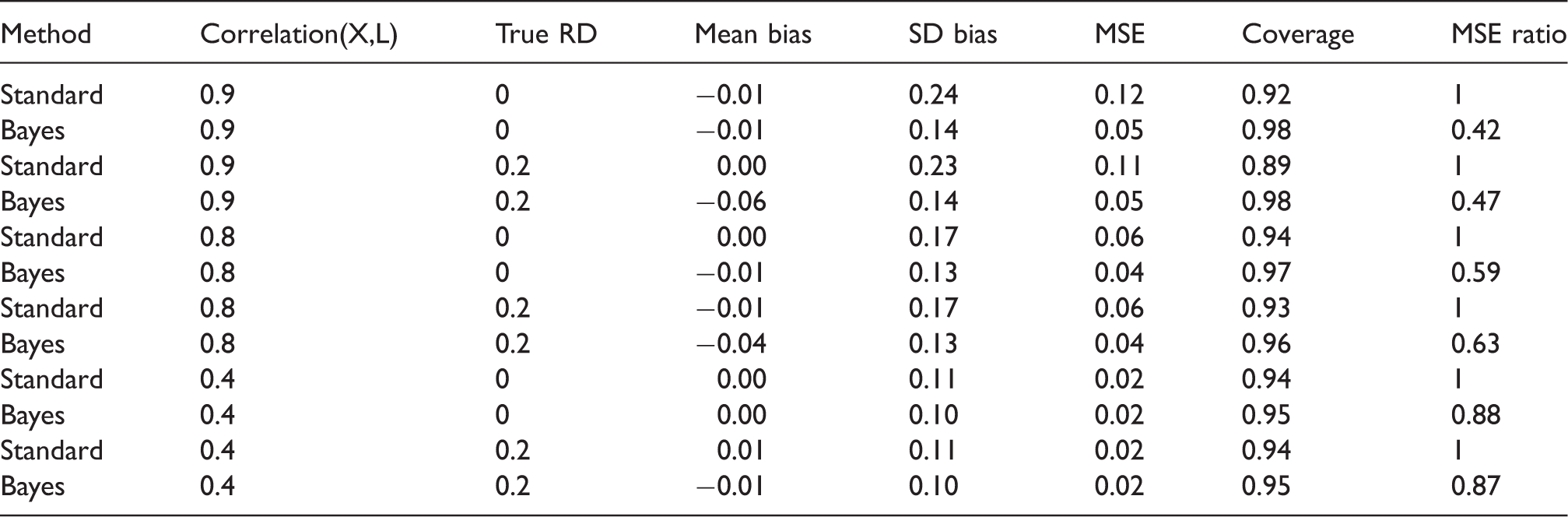
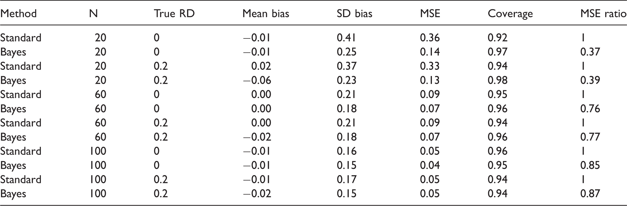
In a time-fixed setting, the standard g-formula requires only a single model to predict the outcome (if we take $p (ℓ | η)$ to be the empirical distribution of L). For both the standard and the Bayesian g-formula, we predict Y using a logistic model with terms for $X, and L$ , with coefficients β. For the model intercept, we used a vague prior with a normal distribution with a mean of log(0.5) and a variance of 1000 ( $N (log (0.5), 1000)$ ). Other coefficients were given identical prior distributions of $β \sim N (0, 3)$ (null, moderately informative priors). We also report MSE as a function of the prior variance on β, where we consider variances corresponding to upper 95% prior-odds ratios of 1.5, 3, 10, 30, 80, and 500.

As expected, the bias was larger for the Bayesian g-formula than for the standard g-formula (Table 1). The sample variance was higher for the standard g-formula estimator, however. With respect to MSE, the Bayesian g-formula under moderately informative priors outperformed the standard g-formula at correlation coefficients of 0.8 and 0.9, and 0.4. Credible interval coverage was, in general, conservative, while confidence interval coverage in the standard g-formula was anticonservative at higher values of the correlation coefficient. Overly precise, null-centered prior information can lead to overshrinkage when the true risk difference is nonnull, in which the MSE starts to increase as one posits increased precision (decreased variance) for the prior distributions of β for the Bayesian g-formula. For example, the minimum MSE for a risk difference of 0.2 occurred at a prior variance of 0.3. At prior variances larger than 0.3, the MSE increases due to larger posterior variance of the risk difference. At prior variances smaller than 0.3, the MSE increases due to larger bias in the posterior mean of the risk difference. When the true risk difference is null, decreasing prior variance leads to vanishing MSE because null values for individual coefficients in the Bayesian g-formula imply a null value for the posterior risk difference (Figure 1).

Figure 1.

Mean-squared error for the risk difference as a function of correlation between X and L and of the prior variance on regression coefficients (log-odds ratios) for simulation given in Section 4.1.

Table 1.

Simulation scenario 1: Two correlated exposures, one time-fixed confounder model intercept priors were vague ( $N (\ln (0.5), 1000)$ ) and other coefficients were null centered and moderately informative ( $N (0, 3)$ ).

Method	Correlation(X,L)	True RD	Mean bias	SD bias	MSE	Coverage	MSE ratio
Standard	0.9	0	−0.01	0.24	0.12	0.92	1
Bayes	0.9	0	−0.01	0.14	0.05	0.98	0.42
Standard	0.9	0.2	0.00	0.23	0.11	0.89	1
Bayes	0.9	0.2	−0.06	0.14	0.05	0.98	0.47
Standard	0.8	0	0.00	0.17	0.06	0.94	1
Bayes	0.8	0	−0.01	0.13	0.04	0.97	0.59
Standard	0.8	0.2	−0.01	0.17	0.06	0.93	1
Bayes	0.8	0.2	−0.04	0.13	0.04	0.96	0.63
Standard	0.4	0	0.00	0.11	0.02	0.94	1
Bayes	0.4	0	0.00	0.10	0.02	0.95	0.88
Standard	0.4	0.2	0.01	0.11	0.02	0.94	1
Bayes	0.4	0.2	−0.01	0.10	0.02	0.95	0.87

MSE: mean-squared error.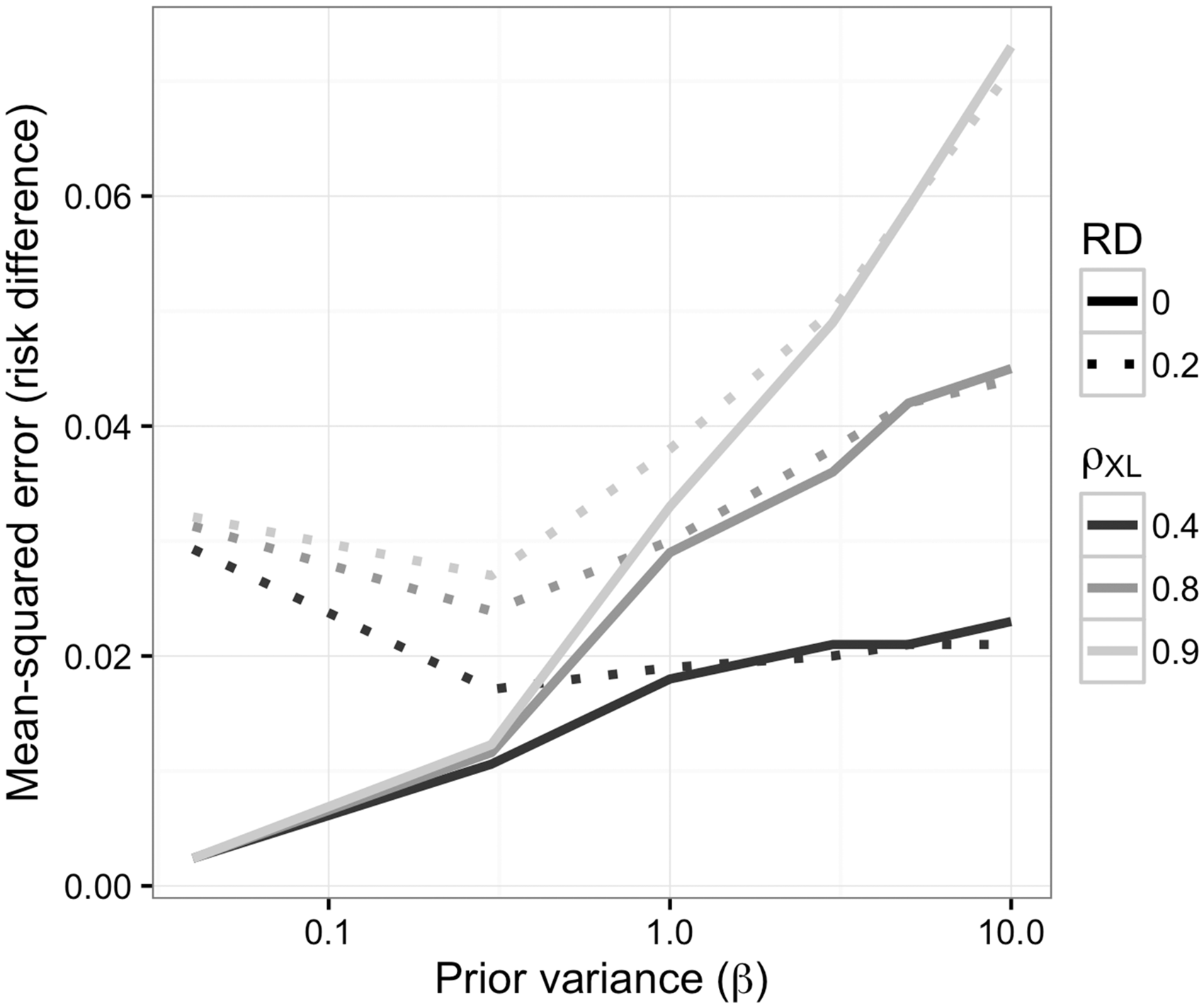

4.2 Time-varying example

We simulate a simple dataset with a time-varying exposure. The data, collected at two time points, $t = (0, 1)$ , include a binary outcome measured at the end of follow up Y(1), a binary exposure at two time points ${X (0), X (1)}$ , and a binary confounder of the exposure–outcome relationship that is also affected by prior exposure L(1). L(1) is related to the outcome by the common cause U, which we consider to be unmeasured. This particular simulation setup has been used previously to illustrate other causal inference methods.²⁶ It addresses a central feature of the Bayesian g-formula: control of confounding by covariates that may also be affected by exposure.

The data are simulated as follows:

$U \sim uniform (0.4, 0.5)$ ;

$X (0) \sim Bernoulli (0.5)$ ;

$L (1) \sim Bernoulli ({logit}^{- 1} (- 1 + X (0) + U))$ ;

$X (1) \sim Bernoulli ({logit}^{- 1} (- 1 + X (0) + L (1)))$ ;

$Y \sim Bernoulli (U + (X (0) + X (1)) / 2 * {rd}^{(\bar{1}, \bar{0})})$ .

In a time-varying setting, the parametric g-formula requires a model to predict L(1) and Y(1). For both the standard and the Bayesian g-formula, we use the correct model (i.e. the logistic model implied by the data-generating mechanism) to predict L(1) (with coefficients η) and we predict Y(1) using a logistic model with terms for $X (0), X (1), and L (1)$ , with coefficients β. All model coefficients were given normal priors ( $N (\ln (0.5), 1000)$ for intercepts and $β, η \sim N (0, 3)$ for all other coefficients). Each analysis was repeated under a true risk difference of 0 and 0.2. We also report MSE as a function of the prior variance on $(β, η)$ , where we consider variances corresponding to upper 95% prior-odds ratios of 1.5, 3, 10, 30, 80, and 500.

As in our time-fixed simulations, under moderately informative, null priors, the bias was larger and the sample variance was smaller for the Bayesian g-formula than for the standard g-formula. In the samples we examined, the Bayesian g-formula outperformed the standard g-formula with respect to MSE (Table 2). As in the previous example, at increasingly higher precision of prior information, the MSE for the Bayesian g-formula can increase as a result of overshrinkage (Figure 2). Unlike the simulation shown in Figure 1, there is no inflection point for which a decrease or increase in prior variance will lead to an increase in the MSE. This is likely due to the small number of values we used for the prior variance, and we speculate that MSE reaches a minimum at some prior variance between 0.04 and 0.3.

Figure 2.

Mean-squared error as a function of sample size and the prior variance on regression coefficients for simulation given in Section 4.2.

Table 2.

Simulation scenario 2: One exposure, one time-varying confounder that depends on exposure. Model intercept priors were vague ( $N (\ln (0.5), 1000)$ ) and other coefficients were null centered and moderately informative ( $N (0, 3)$ ).

Method	N	True RD	Mean bias	SD bias	MSE	Coverage	MSE ratio
Standard	20	0	−0.01	0.41	0.36	0.92	1
Bayes	20	0	−0.01	0.25	0.14	0.97	0.37
Standard	20	0.2	0.02	0.37	0.33	0.94	1
Bayes	20	0.2	−0.06	0.23	0.13	0.98	0.39
Standard	60	0	0.00	0.21	0.09	0.95	1
Bayes	60	0	0.00	0.18	0.07	0.96	0.76
Standard	60	0.2	0.00	0.21	0.09	0.94	1
Bayes	60	0.2	−0.02	0.18	0.07	0.96	0.77
Standard	100	0	−0.01	0.16	0.05	0.96	1
Bayes	100	0	−0.01	0.15	0.04	0.95	0.85
Standard	100	0.2	−0.01	0.17	0.05	0.94	1
Bayes	100	0.2	−0.02	0.15	0.05	0.94	0.87

MSE: mean-squared error; RD: marginal risk difference comparing ‘always exposed’; SD: standard deviation.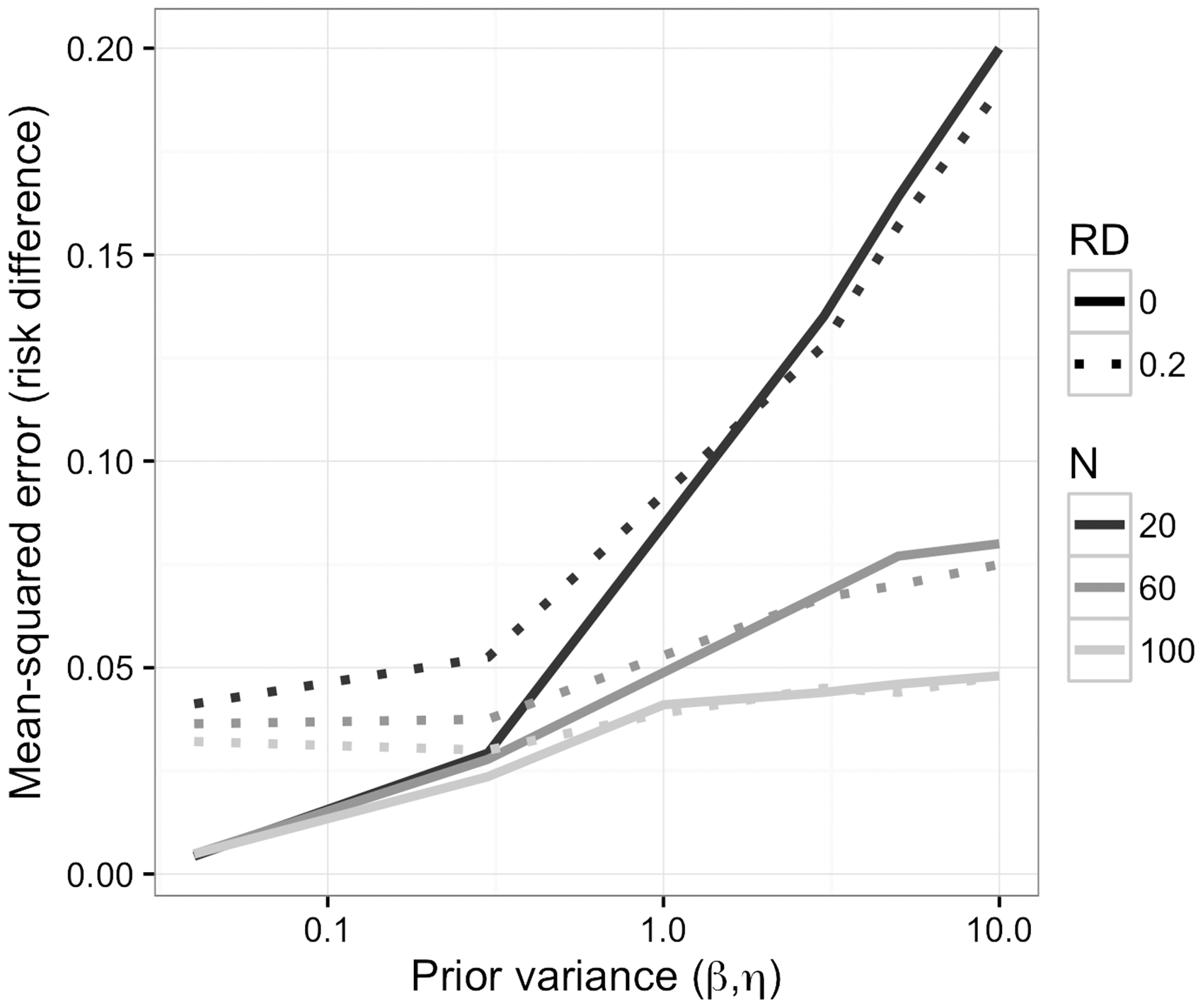

5 Application

We estimated the impact of interventions on environmental tobacco smoke (ETS) on childhood BMI z-scores in a prospective birth cohort. Here we propose to estimate the effects of an intervention that could affect smoking without otherwise influencing BMI (to reiterate, the intervention is assumed to be an instrument for environmental tobacco smoke exposure with respect to BMI). The Mount Sinai Children’s Environmental Health and Disease Prevention Research Center enrolled 479 primiparous women with singleton pregnancies in New York City between 1998 and 2002. The final cohort consists of 404 mother–infant pairs who met previously described inclusion criteria.²⁷ Children were invited to attend follow-up visits at approximately 4–5.5, 6–6.5, and 7–9 years of age (hereafter referred to as visits 1, 2, and 3, respectively) and 69 children attended all three visits. For simplicity, we assume that loss to follow-up is missing completely at random. Maternal baseline characteristics were ascertained via questionnaire at enrollment. At each follow-up visit, we calculated age- and sex-standardized BMI z-scores and classified children as physically active or inactive as described by Buckley et al.²⁸

We estimated posterior distributions for the BMI z-score using the Bayesian g-formula approach. Our specific approach involved a pooled-logistic model for physical activity and a pooled-linear model for the BMI z-score. The predictors in the physical activity model included all baseline covariates (maternal age (quadratic polynomial), maternal prepregnancy BMI (quadratic polynomial), maternal height (linear), smoking during pregnancy (yes, no), race (white, black, or other), education (some high school, high school grad, some college, college grad)) as well as time-varying covariates for cumulative number of visits at which physical activity was reported (lagged one visit, range 0–2), cumulative visits at which ETS was reported (lagged one visit, range 0–2), child’s age (months), and product terms for cumulative ETS and all other variables. The model for BMI z-score used identical predictors and additional terms for current ETS, cumulative years of ETS, and current PA.

For the physical activity model, we used moderately informative priors with 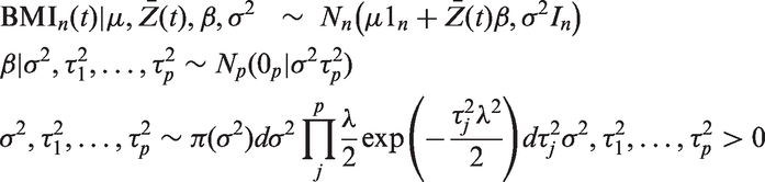$N (0, 3)$ distributions for all covariates, which represent a moderate skepticism that we captured any strong predictor of PA. For the BMI z-score model, we used a Bayesian LASSO approach similar to that of Park and Casella.¹⁸ Briefly, this approach utilizes a double exponential prior, assuming all regression coefficients are exchangeable. This approach differs from placing normally distributed priors on the coefficients in that it places much of the prior mass at the mean. We specified that the prior distribution for each parameter had a mean zero, again suggesting prior skepticism that any particular predictor of BMI z-score is strong. The motivation for using the Bayesian LASSO was both to demonstrate that hierarchical models may be used in the Bayesian g-formula approach as well as that the hierarchical LASSO approach allows the data to inform the amount of shrinkage that occurs (we allow that alternative prior structures may also have this property). The model for the BMI z-score at time t using the Bayesian LASSO has the following hierarchical representation (the justification of which is given in Section 5 of Park and Casella¹⁸)

\begin{matrix} {BMI}_{n} (t) | μ, \bar{Z} (t), β, σ^{2} \sim N_{n} (μ 1_{n} + \bar{Z} (t) β, σ^{2} I_{n}) \\ β | σ^{2}, τ_{1}^{2}, \dots, τ_{p}^{2} \sim N_{p} (0_{p} | σ^{2} τ_{p}^{2}) \\ σ^{2}, τ_{1}^{2}, \dots, τ_{p}^{2} \sim π (σ^{2}) d σ^{2} Π_{j}^{p} \frac{λ}{2} exp (- \frac{τ_{j}^{2} λ^{2}}{2}) d τ_{j}^{2} σ^{2}, τ_{1}^{2}, \dots, τ_{p}^{2} > 0 \end{matrix}

where

\bar{Z} (t)

denotes the n × p matrix of model covariates at time t and τ_p are the elements of a diagonal p × p matrix. We placed an inverse Gamma distribution prior IG(1, 10) on

σ^{2}

, a Gamma distribution prior G(1, 1) on

λ^{2}

, and μ was given an independent, flat prior. We note that the LASSO parameter

(λ)

is not fixed, which allows the data and model to inform the degree to which the β parameters are shrunk toward 0.

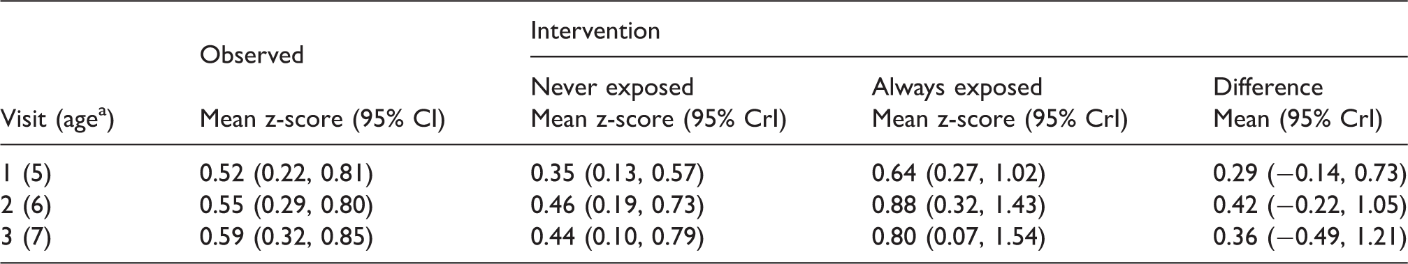
A linear model for the BMI z-score is standard in the literature. We assessed the fit of a linear model for the BMI z-score using the White test for heteroscedasticity,²⁹ which yielded an Lagrange multiplier statistic of 207 (p = 0.45). A plot of standardized residuals versus the predicted BMI z-score is given in Figure 3. For visits 1, 2, and 3, we estimated the median BMI z-score under the interventions “always exposed to ETS” and “never exposed to ETS,” as well as the difference in the mean BMI z-score under these interventions. We report the median of the posterior distribution of the population mean BMI z-score under each intervention (reported as “mean” or “mean z-score”). We report the 2.5th and 97.5th percentile of the posterior distributions as 95% credible intervals.

Figure 3.

Pearson residuals versus predicted BMI z-score from the linear model to predict BMI z-score in the example given in Section 5. Dashed line represents a LOESS line of fit to the data shown in the figure. BMI: body mass index; LOESS: LOcal regrESSion.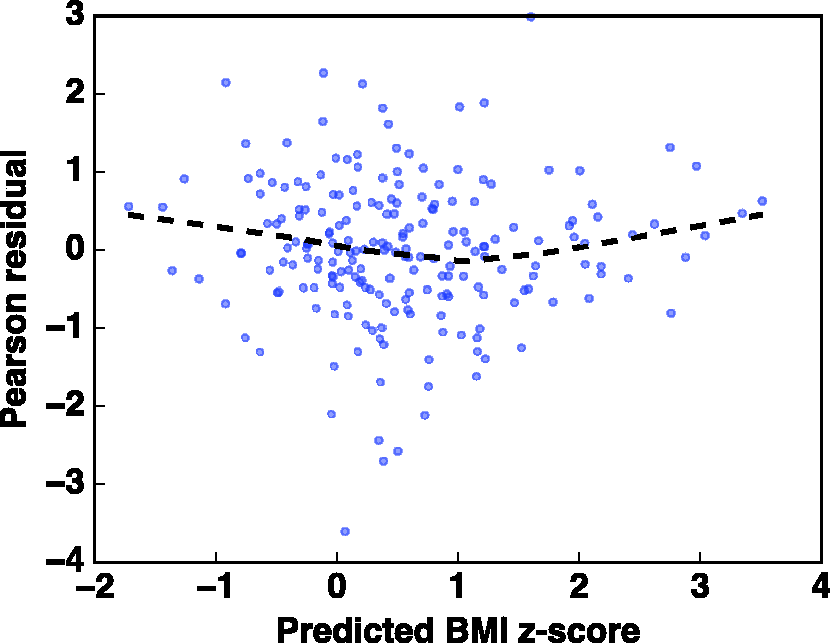

Approximately 25% of the children were exposed to ETS at visit 1, and this proportion increased to 35% at visits 2 and 3. The average BMI observed among the children in the study was slightly above the age-specific population norms, with mean z-scores between 0.5 and 0.6 at visits 1, 2, and 3 (Table 3). At all ages, we estimated that the BMI z-score was higher in the “always exposed” intervention group compared with the “never exposed” intervention group. Comparing the BMI z-score in the always exposed to never exposed (referent), the difference in the mean BMI z-score was largest at visit 2 (posterior median [95% CrI] = 0.42 [−0.22, 1.05]), though the credible intervals included the null at all ages. Our results suggest that environmental tobacco smoke is associated with higher BMI z-score throughout childhood, though the small study size precludes precise estimation in the study population.

Table 3.

Comparing childhood BMI z-scores after potential interventions on environmental tobacco smoke exposure in 69 children, New York, USA, 2004–2008.

	Observed	Intervention
		Never exposed	Always exposed	Difference
Visit (age^a)	Mean z-score (95% CI)	Mean z-score (95% CrI)	Mean z-score (95% CrI)	Mean (95% CrI)
1 (5)	0.52 (0.22, 0.81)	0.35 (0.13, 0.57)	0.64 (0.27, 1.02)	0.29 (−0.14, 0.73)
2 (6)	0.55 (0.29, 0.80)	0.46 (0.19, 0.73)	0.88 (0.32, 1.43)	0.42 (−0.22, 1.05)
3 (7)	0.59 (0.32, 0.85)	0.44 (0.10, 0.79)	0.80 (0.07, 1.54)	0.36 (−0.49, 1.21)

BMI: body mass index; CI: confidence interval; CrI: credible interval.

Mean age at visit.

Using a standard linear regression model adjusted for age and all baseline variables, we estimated that the BMI z-score at each visit was 0.15 higher among those actively exposed to ETS than among those not exposed (95% confidence intervals = −0.20, 0.49). After also adjusting for physical activity, this association increased to 0.22 (95% confidence intervals = −0.12, 0.57). The regression results do not correspond to potential interventions, as in the Bayesian g-formula and so the two results are difficult to compare directly. We note that the magnitude of association was smaller in the regression analysis. In the regression models, we can potentially capture an unbiased estimate of the association between BMI and the ETS behavior reported at the current visit. Thus, this regression model does not capture potential cumulative effects of ETS exposure at prior ages. We fit a model using cumulative ETS exposure, but this model may be subject to uncontrolled confounding by physical activity. After adjusting for physical activity, our estimate could be interpreted (under the assumptions outlined in Appendix 1) as a cumulative direct effect of ETS on BMI that does not operate through physical activity. Further, if there is effect measure modification by physical activity on the absolute scale, then the adjusted regression estimates will not have an easily defined interpretation with respect to informing interventions.

While our results should be seen as primarily illustrative, they show that the effects of interventions on childhood risk factors for obesity can be estimated using standard epidemiologic data, provided that the interventions act as instruments for exposure (a “no side effects” or “treatment-version irrelevance” assumption³⁰). Such inference is valuable in placing the results of observational studies in real-world contexts to prioritize public health actions. We could easily compare the benefits of interventions on smoking to the benefits of interventions on physical activity or diet, for example.¹⁴ Such comparisons are difficult with standard regression approaches, even under conditions in which estimators from regression models are unbiased.

One potential weakness of the Bayesian LASSO approach is that we assume that all model coefficients are exchangeable. It is likely that prior BMI is a much stronger predictor of current BMI than the other confounders considered, so future applications of the Bayesian g-formula could implement nonparametric Bayesian approaches that allow coefficients to shrink to different means. To assess whether our results might be sensitive to the shape of the LASSO prior, we estimated the risk difference using null-centered, normal variables ( $N (0, 3)$ ) in the model for the BMI z-score. The new priors resulted in changes to the risk difference at each visit of less than 0.03 (7%), and results were slightly more precise. Thus, even with the limitations of our illustrative approach, our results appear to be robust to a reasonable range of priors. We also examined the prior predictive distribution of the mean difference (which can be sampled from by removing the likelihood from the algorithm given in Section 3), which was diffuse and did not suggest a strong influence on the posterior.

6 Discussion

From a Bayesian perspective, the g-formula is a natural approach to causal inference. The frequentist version of the g-formula uses the basic rules of probability calculus, along with the language of counterfactuals and explicit identification assumptions, to make inference on the effects of treatment regimes or interventions. Other studies investigating postnatal exposure to environmental tobacco smoke in relation to child body size have also reported positive associations.^31–34 For example, in the Menorca subcohort of the Spanish INMA study, children living with one or two smoking parents at age four years had higher BMI z-scores at ages 4–14 years.³³ BMI z-scores were on average 0.21 (−0.05 to 0.48) or 0.27 (−0.07 to 0.61) units higher among children living with one or two smoking parents compared to nonsmoking parents, respectively.

The observed reduction of the MSE makes the Bayesian g-formula attractive for data analysis from a frequentist perspective. Our simulations suggest that, even in a limited longitudinal setting, default shrinkage priors on conditional model coefficients can result in improved frequentist results for marginal, population parameters (for whom the prior is a complex function of the model parameters and target population covariate distribution). Overshrinkage can result in an increase in the MSE, as well. Our example in Section 5 shows that the Bayesian g-formula is useful in the epidemiologic setting that originally motivated the g-formula: longitudinal data in which exposures, covariates, and outcomes vary over time.³ The approach is useful for making easily interpretable inference, even when data or the relationships between variables are highly complex. Thus, the results are easily communicated with stakeholders, public agencies, and nonstatisticians.

Our approach has much in common with recent examples of Bayesian causal inference and Bayesian predictive inference. Namely, Arjas and coauthors developed an approach analogous to the Bayesian g-formula under a causal framework that does not utilize potential outcomes (described in a general setting in Arjas and Parner⁹ and under a Bayesian framework in Chapter 7 of Berzuini et al.,³⁵ with a practical example given in Arjas and Saarela³⁶ and Saarela et al.³⁷). Robins and Greenland³⁸ refer to the approach that does not utilize the language of potential outcomes as an “agnostic” causal model. In contrast, our approach is derived under the original causal framework of Rubin,²² which bases causal inference on the concept of potential outcomes. The approach of Chib¹⁰ is identical to the g-formula in the time-fixed setting. A previous example by Wang et al.¹³ used the Bayesian g-formula to estimate the effect of a change in ventilation practices on survival in patients with acute lung injury. Notably, none of the examples mentioned focused on Bayesian inference as a way to improve the frequentist performance of causal inference methods. Using our general framework, we build on these applications by integrating the Bayesian Lasso, which demonstrates the potential utility of our approach to use other shrinkage or dimension reduction procedures to improve causal inference. The modularity of our approach allows for the straightforward incorporation of other Bayesian regression solutions to problems such as inference with highly correlated covariates⁴ or accounting for measurement error.⁸

As we show, Bayesian causal inference can be framed as a prediction problem. De Los Campos et al.³⁹ previously used a Bayesian LASSO approach to predict quantitative traits in wheat and mice based on genetic markers. In contrast to their approach, our work frames prediction in terms of causal inference, where the goal is not simply to predict observed outcomes, but to predict such outcomes had we been able to change an exposure or treatment. Interestingly, De Los Campos et al.³⁹ showed that the Bayesian LASSO can be used when the number of parameters exceeds the sample size, a canonical problem in high-dimensional data. Our approach could be used to extend these results to make causal contrasts in higher dimensional problems.

A characteristic feature of our approach is that we do not place priors directly on the quantity of interest. Thus, the bias–variance trade-off of the Bayesian g-formula is not targeted toward the causal estimand. Similar claims can be made about frequentist parametric g-formula. Recent likelihood-based approaches, such as targeted maximum likelihood (minimum loss) estimation (TMLE), remedy this feature of standard causal inference approaches by “targeting” the estimator at the parameter of interest, rather than the nuisance parameters that go into predicting the outcome or the treatment/exposure.⁴⁰ TMLE is typically combined with SuperLearner, which is an ensemble learning approach that averages predictions across many (possibly semiparametric or nonparametric) models.⁴¹ More generally, TMLE falls under the heading of “double-robust” methods, which are consistent if either the outcome model or the treatment/exposure model is correct. Such methods are typically based on restricted-moment models developed in the semiparametric literature,⁴² which do not imply a full likelihood and thus are not easily incorporated into a Bayesian framework. Graham et al.⁴³ used an approach on Bootstrap methods, which has approximate Bayesian inference for the posterior predictive distribution of causal effects. Because such an approach is outside of a formal Bayesian framework, it is difficult to ascertain whether it could easily incorporate other aspects of a formal Bayesian analysis that accounts for problems such as measurement error or missing data. However, it is more robust to model misspecification than our approach. We address this shortcoming by ensuring that the posterior is flexibly parameterized, which allows for a variety of model forms. Thus, the Bayesian g-formula can be cast as one alternative to double-robust estimation as a way to reduce model specification assumptions. Bayesian model averaging⁴⁴ may be an additional way to incorporate robustness to model misspecification in our framework.

In more general settings with higher dimensional data, the need for flexibility grows even further as approximating correct model specification is more difficult. Other causal approaches, such as the use of inverse probability weighting to estimate the parameters of a marginal structural model, can marginalize over some of these parameters. However, such an approach necessitates modeling the (possibly longitudinal) exposure mechanism and a marginal model for the outcome, and thus does not completely absolve one from the modeling task. In some settings, such as studies of occupational exposures where time-varying confounders may have deterministic relationships with the exposure of interest, such alternative approaches may not be possible.⁴⁵ Using multiple causal approaches with different modeling assumptions to answer the same question can help triangulate the effects of interventions. Further work is needed regarding how to select model forms for $p (ℓ (t) | \cdot)$ and $p (y (t) | \cdot)$ because the g-formula estimator is a function of both models. Our work suggests that some model selection choices can be avoided by introducing some flexibility and leveraging the shrinkage properties of Bayesian methods. This shows that previous knowledge about shrinkage estimation in standard regression models⁴⁶ may also apply to causal analysis where the estimator is a complex function of multiple parameters.

One potential concern in using the g-formula is the g-null paradox, in which model misspecification leads to hypothesis tests that inevitably reject the null hypothesis as sample size increases, even when the causal null hypothesis is true.⁴⁷ Part of this paradox is explained by considering that some choices of model form can rule out the null hypothesis a priori because no parameter values in the model parameter space are consistent with the causal null hypothesis—we say that such models are “incompatible.” Similar concerns may arise with prior specifications that rule out the null. Allowing for flexible models increases the parameter space but may necessitate the use of shrinkage priors, which may reduce concern over this paradox in the Bayesian setting, provided that the prior parameter space includes the “g-null” hypothesis. In the Bayesian setting, presence of the g-null paradox can be assessed by examining whether the prior predictive distribution of the potential outcomes (which is a function both of the priors, the intervention, the model, and the target population) rules out the g-null hypothesis. In general, we recommend examining the prior predictive distribution of the marginal parameter of interest to conceptualize how the joint function of the regression priors might influence the marginal parameter of interest in possibly unexpected ways.

We demonstrated that hierarchical modeling is feasible in the Bayesian g-formula, which suggests multiple future directions. Our example leveraged the naturally modular aspect of Bayesian modeling: once a probability model can be used to describe a process (e.g. measurement error, missing data), it is relatively straightforward to include that model as part of a Bayesian hierarchical model. This modular aspect of the Bayesian g-formula opens up many possibilities for improving causal inference in real-world data where some variables are not measured, and those that are measured may be recorded with error.

Footnotes

Declaration of conflicting interests

The author(s) declared no potential conflicts of interest with respect to the research, authorship, and/or publication of this article.

Funding

The author(s) disclosed receipt of the following financial support for the research, authorship, and/or publication of this article: National Institutes of Health Grant # 5T32ES007018-38; The Mount Sinai Children’s Environmental Health Study was supported by NIEHS/EPA Children’s Center grants ES09584 and R827039, The New York Community Trust, and ATSDR/CDC/ATPM.

References

Glass

Goodman

Hernán

et al.

Causal inference in public health. Annu Rev Public Health 2013; 34: 61–75.

Robins

. A new approach to causal inference in mortality studies with a sustained exposure period—Application to control of the healthy worker survivor effect. Math Mod 1986; 7: 1393–1512.

Keil

Edwards

Richardson

et al.

The parametric g-formula for time-to-event data: intuition and a worked example. Epidemiology 2014; 25: 889–897.

MacLehose

Dunson

Herring

et al.

Bayesian methods for highly correlated exposure data. Epidemiology 2007; 18: 199–207.

Thomas

Witte

Greenland

. Dissecting effects of complex mixtures: who’s afraid of informative priors? Epidemiology 2007; 18: 186–190.

Efron

Morris

. Stein’s paradox in statistics. Scientific Am 1977; 236: 119–127.

Stein C, et al. Inadmissibility of the usual estimator for the mean of a multivariate normal distribution. In: Proceedings of the third Berkeley symposium on mathematical statistics and probability. Berkeley, Calif: University of California Press, 1956, vol. 1, pp.197–206.

Keil

Daniels

Hertz-Picciotto

. Autism spectrum disorder, flea and tick medication, and adjustments for exposure misclassification: the CHARGE (CHildhood Autism Risks from Genetics and Environment) case–control study. Environ Health 2014; 13: 889–897.

Arjas

Parner

. Causal reasoning from longitudinal data. Scand J Stat 2004; 31: 171–187.

10.

Chib

. Analysis of treatment response data without the joint distribution of potential outcomes. J Econom 2007; 140: 401–412.

11.

Gustafson

. Discussion of “on Bayesian estimation of marginal structural models.”. Biometrics 2015; 71: 291–293.

12.

Saarela

Stephens

Moodie

et al.

On Bayesian estimation of marginal structural models. Biometrics 2015; 71: 279–288.

13.

Wang

Scharfstein

Wang

et al.

Estimating the causal effect of low tidal volume ventilation on survival in patients with acute lung injury. J R Stat Soc Ser C Appl Stat 2011; 60: 475–496.

14.

Taubman

Robins

Mittleman

et al.

Intervening on risk factors for coronary heart disease: an application of the parametric g-formula. Int J Epidemiol 2009; 38: 1599–1611.

15.

Ahern

Hubbard

Galea

. Estimating the effects of potential public health interventions on population disease burden: a step-by-step illustration of causal inference methods. Am J Epidemiol 2009; 169: 1140–1147.

16.

Westreich

Cole

Young

et al.

The parametric g-formula to estimate the effect of highly active antiretroviral therapy on incident aids or death. Stat Med 2012; 31: 2000–2009.

17.

Keil

Richardson

. Reassessing the link between airborne arsenic exposure among anaconda copper smelter workers and multiple causes of death using the parametric g-formula. Environ Health Perspect 2017; 125: 608–614.

18.

Park

Casella

. The Bayesian lasso. J Am Stat Assoc 2008; 103: 681–686.

19.

Cole

Hudgens

Brookhart

et al.

Risk. Am J Epidemiol 2015; 181: 246–250.

20.

Pearl

. On the consistency rule in causal inference: axiom, definition, assumption, or theorem? Epidemiology 2010; 21: 872–875.

21.

Rosenbaum

. The consequences of adjustment for a concomitant variable that has been affected by the treatment. J R Stat Soc Ser A-G 1984; 147: 656–666.

22.

Rubin

. Bayesian inference for causal effects: the role of randomization. Ann Stat 1978; 6: 34–58.

23.

Edwards

Cole

Westreich

. All your data are always missing: incorporating bias due to measurement error into the potential outcomes framework. Int J Epidemiol 2015; 44: 1452–1459.

24.

Hamra

MacLehose

Cole

. Sensitivity analyses for sparse-data problems-using weakly informative Bayesian priors. Epidemiology 2013; 24: 233–239.

25.

Greenland

Mansournia

. Penalization, bias reduction, and default priors in logistic and related categorical and survival regressions. Stat Med 2015; 34: 3133–3143.

26.

Robins

Hernán

Estimation of the causal effects of time-varying exposures. In: Fitzmaurice

Davidian

Verbeke

et al. (eds). Longitudinal Data Analysis, boca raton: Chapman & Hall/CRC, 2009; Vol. 26: 553–600.

27.

Engel

Berkowitz

Barr

et al.

Prenatal organophosphate metabolite and organochlorine levels and performance on the brazelton neonatal behavioral assessment scale in a multiethnic pregnancy cohort. Am J Epidemiol 2007; 165: 1397–1404.

28.

Buckley

Engel

Mendez

et al.

Prenatal phthalate exposures and childhood fat mass in a New York City cohort. Environ Health Perspect 2015; 124: 507–513.

29.

White

. A heteroskedasticity-consistent covariance matrix estimator and a direct test for heteroskedasticity. Econom J Econom Soc 1980; 48: 817–838.

30.

Cole

Frangakis

. The consistency statement in causal inference: a definition or an assumption? Epidemiology 2009; 20: 3–5.

31.

McConnell

Shen

Gilliland

et al.

A longitudinal cohort study of body mass index and childhood exposure to secondhand tobacco smoke and air pollution: the Southern California children’s health study. Environ Health Perspect 2015; 123: 360–366.

32.

Møller

Ajslev

Andersen

et al.

Risk of childhood overweight after exposure to tobacco smoking in prenatal and early postnatal life. PLoS One 2014; 9: e109184–e109184.

33.

Robinson

Martínez

Aurrekoetxea

et al.

The association between passive and active tobacco smoke exposure and child weight status among Spanish children. Obesity (Silver Spring) 2016; 24: 1767–1777.

34.

Yang

Decker

Kramer

. Exposure to parental smoking and child growth and development: a cohort study. BMC Pediatr 2013; 13: 104–104.

35.

Berzuini

Dawid

Bernardinell

. Causality: statistical perspectives and applications, West Sussex, UK: John Wiley & Sons, 2012.

36.

Arjas

Saarela

. Optimal dynamic regimes: presenting a case for predictive inference. Int J Biostat 2010; 6: 1–21.

37.

Saarela

Arjas

Stephens

et al.

Predictive Bayesian inference and dynamic treatment regimes. Biom J 2015.

38.

Robins

Greenland

. Causal inference without counterfactuals: comment. J Am Stat Assoc 2000; 95: 431–435.

39.

De Los Campos

Naya

Gianola

et al.

Predicting quantitative traits with regression models for dense molecular markers and pedigree. Genetics 2009; 182: 375–385.

40.

van der Laan

Rubin

. Targeted maximum likelihood learning. Int J Biostat 2006; 2: 1–1.

41.

Polley EC and van der Laan MJ. SuperLearner: Super Learner prediction, http://CRAN.R-project.org/package=SuperLearner. R package version 2.0-9, (2012, accessed 8 January 2016).

42.

Tsiatis AA. Semiparametric theory and missing data. Springer Series in Statistics. New York: Springer-Verlag, 2006.

43.

Graham

McCoy

Stephens

. Approximate Bayesian inference for doubly robust estimation. Bayesian Anal 2016; 11: 47–69.

44.

Madigan D, Raftery AE, Volinsky C, et al. Bayesian model averaging. In: Proceedings of the AAAI workshop on integrating multiple learned models, Portland, OR: AAAI Press, 1996, pp.77–83.

45.

Buckley

Keil

McGrath

et al.

Evolving methods for inference in the presence of healthy worker survivor bias. Epidemiology 2015; 26: 204–212.

46.

Greenland

. Principles of multilevel modelling. Int J Epidemiol 2000; 29: 158–167.

47.

Robins

. General methodological considerations. J Econom 2003; 112: 89–106.

48.

Robins

Causal inference from complex longitudinal data. In: Berkane

(ed). Latent variable modeling applications to causality, New York: Springer, 1997; Vol. 120: 69–117.

49.

Young

Cain

Robins

et al.

Comparative effectiveness of dynamic treatment regimes: an application of the parametric g-formula. Stat Biosci 2011; 3: 119–143.