A Bayesian hierarchical model for discrete choice data in health care

Abstract

In discrete choice experiments, patients are presented with sets of health states described by various attributes and asked to make choices from among them. Discrete choice experiments allow health care researchers to study the preferences of individual patients by eliciting trade-offs between different aspects of health-related quality of life. However, many discrete choice experiments yield data with incomplete ranking information and sparsity due to the limited number of choice sets presented to each patient, making it challenging to estimate patient preferences. Moreover, methods to identify outliers in discrete choice data are lacking. We develop a Bayesian hierarchical random effects rank-ordered multinomial logit model for discrete choice data. Missing ranks are accounted for by marginalizing over all possible permutations of unranked alternatives to estimate individual patient preferences, which are modeled as a function of patient covariates. We provide a Bayesian version of relative attribute importance, and adapt the use of the conditional predictive ordinate to identify outlying choice sets and outlying individuals with unusual preferences compared to the population. The model is applied to data from a study using a discrete choice experiment to estimate individual patient preferences for health states related to prostate cancer treatment.

Keywords

Best–worst discrete choice experiment conditional predictive ordinate missing data outliers random effects relative attribute importance

1 Introduction

Discrete choice experiments (DCEs) have been increasingly used in health applications to characterize the preferences of individual patients for various health care interventions and services.^1,2 In a typical health care DCE, patients are presented with sets of health states described by various attributes and asked to make choices from among them.³ For example, a patient might be asked to choose between a health state with long life expectancy and poor quality of life and a health state with shorter life expectancy and high quality of life. By asking individuals to make choices between health states, they are forced to make trade-offs that reveal information about their preferences for different aspects of health-related quality of life.

Historically, in a DCE, patients provided their most preferred health state or a full ranking of a set of possible health states. However, continued research in discrete choice experiments has led to the development of best–worst designs in which patients provide only their most preferred and least preferred choices.^4,5 While reducing patient burden compared to full rankings, best–worst discrete choice experiments pose new statistical challenges. In such data, incomplete ranking information occurs when choosing best and worst from among four or more health states, and patient-level data are often insufficient to estimate individual-level preferences using maximum likelihood methods as it is not uncommon to obtain estimates of the coefficients in the wrong direction with sparse data.^6,7

A number of models have been developed for discrete choice data. The multinomial logit models the probability of observing best choices,⁸ while the rank-ordered logit models the probability of full rankings.⁹ Mixed logit models include random effects that vary across individuals to account for heterogeneity in preferences.^10,11 More recently, Allenby et al. developed a Bayesian hierarchical model for best choices with random effects and individual-level covariates⁶ and Hernandez-Alava et al. introduced a model for ranked and partially ranked data that includes random effects, and estimated the random effects using Monte Carlo maximum likelihood methods.¹² Although the model introduced by Hernandez-Alava et al. accommodates partially ranked data, it is not uncommon to obtain coefficient estimates in the wrong direction when using maximum likelihood estimation with sparse data.⁷ Moreover, their model does not include individual-specific covariates although inference on covariate effects is often of interest and it has been shown that including covariates can improve preference estimates for the mixed logit.^6,13–15

In many studies, a key purpose of the DCE is to obtain an individual’s ranking of various attributes relative to each other. The concept of relative attribute importance is widely used in the marketing research literature to provide rankings of features of consumer products.^16–18 Recently, this concept has been extended into the health care domain.^19–21 In this context, the purpose of the DCE is to obtain an individual’s ranking of various attributes of health care or health-related quality of life, so that this information can be used as part of the health care decision-making process. For example, how a prostate cancer patient values full sexual functioning, long lifespan and no urinary incontinence relative to each other may inform which treatment options are a better match for the patient. While discrete choice data are now routinely analyzed using Bayesian hierarchical models with random effects to accommodate preference heterogeneity,^6,11,22,23 methods to compute relative attribute importance for such models are not fully developed.

Methods to identify outliers for such models are also lacking. Using the means of the individual-specific parameter distributions, Campbell et al.²⁴ classified individuals in the upper and lower percentiles as outliers. Farrel et al.²⁵ proposed a graphical method to identify outliers by plotting standardized random effects against their expected values for a Bayesian hierarchical logistic regression model. Several approaches for outlier detection in Bayesian models have been explored. For example, using the posterior distribution of the residuals of a regression model, Chaloner and Brant²⁶ and Chaloner^27,28 define an outlier as an observation with a large random error and calculate the posterior probabilities that observations are outlying. Other approaches for outlier detection are based on the predictive distribution. The conditional predictive ordinate (CPO), first suggested by Geisser,²⁹ is a diagnostic measure used to detect observations discrepant with the proposed model.^29–34 To our knowledge, CPO has not been used to identify outlying random effects.

In this paper, we develop a Bayesian hierarchical model for best–worst discrete choice data. Our model extends previous approaches. Incomplete rankings are handled by marginalizing over all possible permutations of unranked health states in a model that includes random effects to model individual-specific preferences. Bayesian methods are used to overcome the problem of sparse data to obtain estimates of individual preferences. To enable analysis of how patient characteristics are related to preferences, we model individual-specific preferences as a function of individual-specific covariates. We also define Bayesian versions of relative attribute importance for individuals and for the population that handle random effects and covariates. To identify outliers in DCEs, we adapt the CPO in two ways: we adapt it to include random effects to identify patients who are unusual in their preferences for specific attributes or combinations of attributes, and we adapt it to handle vector outcomes to identify choice sets that are outlying with respect to individual preferences.

The paper is organized as follows. Section 2 describes the motivating dataset and defines terms used throughout the remainder of the paper. Section 3 presents the Bayesian hierarchical model for best–worst choice data with random effects and patient covariates. Section 4 defines measures of relative importance, while Section 5 presents CPO-based measures for outlier detection. Section 6 demonstrates application of our methods to data from the PROSPECT study. This is followed by a discussion in Section 7.

2 Motivating example: the PROSPECT study

The methods are motivated by the PROSPECT (PROState cancer PrEferenCes for Treatment) study, which used a DCE to understand patient preferences for aspects of health-related quality of life associated with prostate cancer treatment outcomes.³⁵ The 121 patients were men with negative prostate biopsies.

We make the following definitions. An attribute is a characteristic of a treatment or a health state resulting from a treatment. For simplicity of discussion, we define an attribute as a characteristic of a health state. Attributes are defined by at least two attribute levels. For example, sexual functioning is an attribute with three attribute levels, no sexual functioning, decreased sexual functioning and full sexual functioning. Investigators identified seven attributes important for prostate cancer treatment decision-making using a “voice of the patient” process.³⁵ In addition to sexual functioning, these were urinary incontinence, bowel issues, expected lifespan, others’ support for the proposed treatment, and cutting and taking immediate action towards treatment. Table 1 presents the seven attributes with their attribute levels. Health state attribute variables are dummy variables for health state attributes with the lowest attribute level as the reference group. A health state is defined by specifying attribute levels for each of the seven attributes. Sets of health states from which patients make choices are called choice sets and a health state contained in a choice set is called an alternative. An example of a choice set is shown in Figure 1.

Table 1.

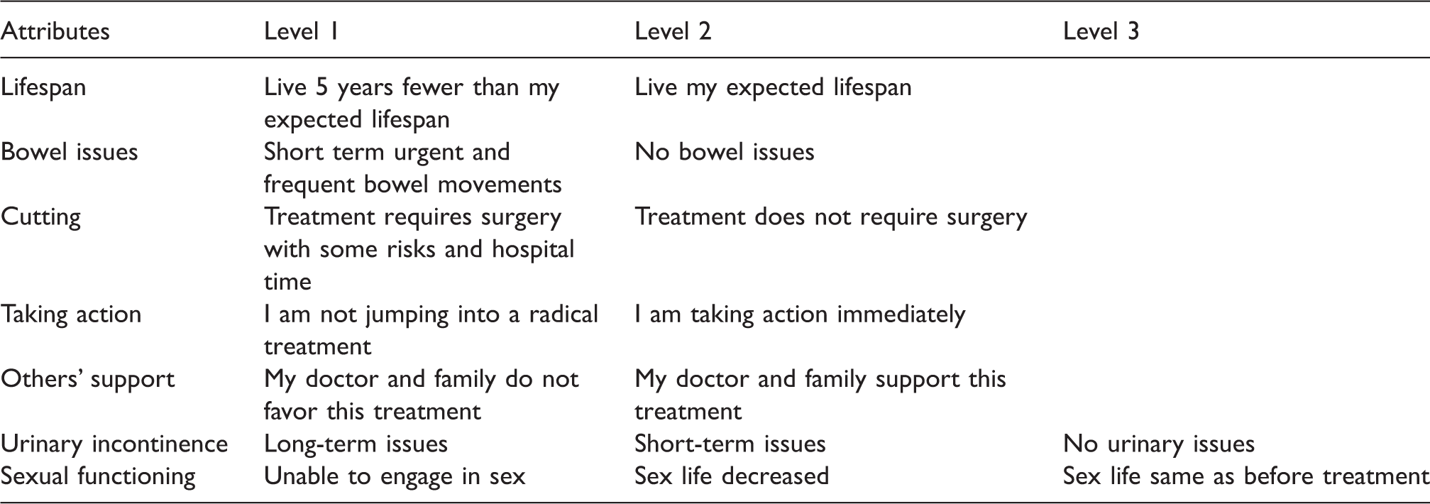
Attributes and attribute levels from the PROSPECT Study.

Attributes	Level 1	Level 2	Level 3
Lifespan	Live 5 years fewer than my	Live my expected lifespan
	expected lifespan
Bowel issues	Short term urgent and	No bowel issues
	frequent bowel movements
Cutting	Treatment requires surgery	Treatment does not require surgery
	with some risks and hospital
	time
Taking action	I am not jumping into a radical	I am taking action immediately
	treatment
Others’ support	My doctor and family do not	My doctor and family support this
	favor this treatment	treatment
Urinary incontinence	Long-term issues	Short-term issues	No urinary issues
Sexual functioning	Unable to engage in sex	Sex life decreased	Sex life same as before treatment

Figure 1.

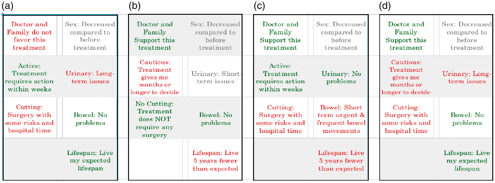
Example of a choice set from the PROSPECT study. Patients choose their most and least preferred health state from among the four health states.

In the PROSPECT study, patients were presented with choice sets comprised of four hypothetical health states that could result from various cancer treatments, and asked to choose their most and least preferred health state from each set, leaving two health states unranked. Sixteen health states were selected by investigators for creation of choice sets. These sixteen health states described by their attribute levels are presented in Table 6, Appendix 1. The first four choice sets were the same for all patients and consisted of health states {1,3,9,15}, {2,4,10,14}, {5,6,11,12} and {7,8,13,16}. An algorithm was used to create the remaining choice sets for each patient. The algorithm composed subsequent choice sets in a manner that achieved an implicit ranking of the 16 states using the minimum of choice sets. As a result, the number of choice sets as well as the choice sets presented to each patient differed. The number of choice sets per patient ranged from 10 to 17.

3 Bayesian hierarchical model for best–worst choice data

Our model includes a probability model for best–worst choice data with incomplete rankings, a hierarchical prior distribution, and individual-specific covariates predicting an individual’s preference scores for attributes.

3.1 Probability model

Let $i = 1, \dots, N$ index patients, $t = 1, \dots, T_{i}$ index choice sets within patient i, and $j = 1, \dots, J_{it}$ index health states within choice set t presented to patient i, where N is the total number of patients, T_i is the total number of choice sets presented to patient i, and J_it is the total number of health states in choice set t presented to patient i.

Let $Y_{it}$ be a $J_{it} \times 1$ vector describing an observed full ranking of a choice set, where element y_itj of $Y_{it}$ is the observed jth ranked health state in choice set t presented to individual i. For example, in the PROSPECT study, all patients are presented with multiple choice sets of size J_it = 4 and the total number of choice sets presented to each patient T_i varied among patients. Suppose patient i gives a full ranking $D > A > C > B$ of choice set $t = {A, B, C, D}$ where D is most preferred and B is least preferred. Then $Y_{it} = (y_{it 1}, y_{it 2}, y_{it 3}, y_{it 4}) T = (D, A, C, B) T$ .

We use a linear predictor³⁶ to relate choices to the attribute levels of health states. Let $x_{itj}$ be an $H \times 1$ vector encoding the attribute levels of the jth ranked health state in choice set t presented to individual i, where H is the total number of health state attribute variables. Let $β_{i}$ be an $H \times 1$ unknown vector of preference scores for individual i.

Suppose that individual i provides only a most preferred health state for choice set t. Then the probability that individual i chooses the jth health state as the best state in choice set t is

p (y_{itj} | β_{i}) = \frac{\exp (x_{itj}^{T} β_{i})}{\sum_{k = 1}^{J_{it}} \exp (x_{itk}^{T} β_{i})}

(1)

where the summation is over the health states in the choice set.⁸

Patient i is presented with T_i choice sets, each of size J_it = 4. Eliciting the best and worst choices from a choice set of size 4 yields a partial ranking of the choice set. Two possible full rankings are consistent with each partial ranking. For example, the full rankings $A > B > C > D$ and $A > C > B > D$ are consistent with the partial ranking $A > {B, C} > D$ , where A is the most preferred and D is the least preferred. We can model the probability of observing a full ranking of health states as a product of probabilities, where each factor in the product is the probability of observing a best choice from a subsequently smaller choice set. For example, the probability of observing the full ranking $A > B > C > D$ is the product of the probability of choosing A as best from the choice set ${A, B, C, D}$ times the probability of choosing B as best from the choice set {B, C, D} times the probability of choosing C as best from the choice set {C, D}. The probability of choosing D from {D} is one.

Let $r = 1, \dots, R_{it}$ index the full rankings consistent with an elicited partial ranking of choice set t for patient i, where R_it is the total number of possible full rankings consistent with the partial ranking. Then the probability of observing $Y_{rit}$ , a full ranking consistent with the partial ranking $Y_{it}$ , is written as the probability of a sequence of choices^5,37,38

p (Y_{rit} | β_{i}) = Π_{j = 1}^{J_{it} - 1} \frac{\exp (x_{ritj}^{T} β_{i})}{\sum_{J_{it} \geq k \geq j} \exp (x_{ritk}^{T} β_{i})}

(2)

Because the set of R_it full rankings consistent with $Y_{it}$ is a set of mutually exclusive events, marginalizing over all possible permutations of unranked health states amounts to summing over all possible full rankings, and the probability of observing a partial ranking $Y_{it}$ is

p (Y_{it} | β_{i}) = \sum_{r = 1}^{R_{it}} (Π_{j = 1}^{J_{it} - 1} \frac{\exp (x_{ritj}^{T} β_{i})}{\sum_{J_{it} \geq k \geq j} \exp (x_{ritk}^{T} β_{i})})

(3)

If a patient is asked to provide their most preferred and least preferred health states from a choice set t containing fewer than four alternatives or if choice set t is fully ranked, then equation (3) simplifies to equation (2). Moreover, if we observe only best choices, then equation (3) simplifies to equation (1).

Let $Y_{i} = {Y_{i 1}, \dots, Y_{{iT}_{i}}}$ represent the set of partial rankings made by patient i over the course of the experiment. Then assuming that each set of rankings $Y_{it}$ is conditionally independent given $β_{i}$ , the likelihood contribution for individual i is given by

p (Y_{i} | β_{i}) = Π_{t = 1}^{T_{i}} p (Y_{it} | β_{i})

(4)

3.2 Hierarchical prior distributions

Let $z_{i}$ be a $Q \times 1$ vector of patient covariates for individual i including an intercept. For example, suppose we want to include an indicator for patient age greater than 65 years in the model. Then we could let $z_{i} = (1, z_{i 1}) T$ where $z_{i 1} = 1$ when patient age is greater than 65 and $z_{i 1} = 0$ otherwise. To model patient preferences as a function of patient covariates, we model random effect $β_{i}$ as a linear function of $z_{i}$ plus error as

β_{i} = Γ z_{i} + ε_{i}

(5)

where

Γ

is an unknown H × Q matrix of fixed regression coefficients and

ε_{i}

is an

H \times 1

mean zero random effect vector that allows patients with the same covariates to have different values for

β_{i}

. We model

ε_{i}

ε_{i} | Σ \sim {Normal}_{H} (0, Σ)

(6)

a multivariate normal distribution with mean vector 0 and H × H covariance matrix

Σ

. Let

h = 1, \dots, H

index health state attribute variables, and

q = 1, \dots, Q

index patient covariates. Then each element γ_hq of

Γ

describes the effect of covariate q on patient preference for attribute variable h. We set the prior for the γ_hq as

γ_{hq} \sim Normal (0, 1)

(7)

and the prior for

Σ

Σ \sim inverseWishart (w, W)

(8)

an inverse Wishart distribution with w degrees of freedom and scale matrix W . We set the prior mean of the inverse Wishart distribution equal to the identity matrix. If no covariates are included, then equation (5) reduces to

β_{i} = μ + ε_{i}

, where

μ = (μ_{h})

is the

H \times 1

unknown population mean vector of the distribution of

β_{i}

. In this case, we set a prior for

μ

μ \sim {Normal}_{H} (0, I_{H})

, where 0 is the

H \times 1

zero vector and

I_{H}

is the H × H identity matrix.

4 Relative attribute importance

An attribute may be represented using two, three or more levels. When using dummy variable coding, this yields one, two or more coefficients where the coefficient for the reference level is defined to be zero. In market research, the difference between the estimated maximum and minimum attribute-level coefficients has been used as a measure of attribute importance.^16–18 Relative attribute importance is calculated by normalizing attribute importance measures to sum to one, so that the relative importance of an attribute is a proportional contribution to the importance of all attributes jointly.³⁹ Although model coefficients can be estimated using maximum likelihood or Bayesian methods,¹⁸ current methods only provide point estimates of relative importance. We extend current measures by defining relative attribute importance as a function of the random effects $β_{i}$ , and describe Bayesian versions of relative attribute importance.

Let $a = 1, \dots, A$ index health state attributes, where A is total number of health state attributes and let $k = 1, \dots, K_{a}$ index the attribute levels of attribute a, where K_a is the total number of attribute levels for attribute a. In the PROSPECT study, we consider seven health state attributes. Urinary functioning and sexual functioning each have three attribute levels, while the other attributes have two levels. The importance of attribute a for individual i is defined as

max_{k} β_{iak} - min_{k} β_{iak}

where β_iak is an unknown preference score for the k ^th attribute level within attribute a for patient i. Using equation (5), we define the relative importance (RI) of attribute variable a for individual i as the proportional contribution of attribute variable A to the sum of all attributes’ importance

{RI}_{ia} = \frac{max_{k} (γ_{ak}^{T} z_{i} + ε_{iak}) - min_{k} (γ_{ak}^{T} z_{i} + ε_{iak})}{\sum_{f = 1}^{A} max_{k} (γ_{fk}^{T} z_{i} + ε_{ifk}) - min_{k} (γ_{fk}^{T} z_{i} + ε_{ifk})}

(9)

where

γ_{ak}^{T}

is the row of

Γ

corresponding to attribute level k within attribute a, and ε_iak is the random effect for the k ^th attribute level within attribute a for individual i. If no patient covariates are included in the model, then

γ_{ak}^{T} z_{i}

reduces to μ_ak, the k ^th attribute level population preference score within attribute a for attribute a.

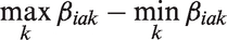
We can define the average relative importance (ARI) of attribute a for the population as the arithmetic average of equation (9) over all patients

{ARI}_{a} = \frac{1}{N} \sum_{i = 1}^{N} {RI}_{ia}

(10)

For a specific set of patient covariates z , we define the relative importance of attribute a for the population as

{RI}_{az} = \frac{max_{k} (γ_{ak}^{T} z) - min_{k} (γ_{ak}^{T} z)}{\sum_{f = 1}^{A} max_{k} (γ_{fk}^{T} z) - min_{k} (γ_{fk}^{T} z)}

(11)

where the summation is over all attributes. This formulation can be used to, for example, compute marginal predictions at specific patient covariate values. If no patient covariates are included in the model, then

γ_{ak}^{T} z

reduces to μ_ak and we get estimates of relative importance at the population level.

Equation (11) differs from equation (10) in that relative importance is calculated from population parameters, rather than as an average of the individual preference scores.

The posterior means and standard deviations of equations (9) to (11) are estimated as the means and standard deviations of the MCMC samples of relative importance scores, calculated using randomly sampled draws from the posterior distributions of the relevant parameters.

5 Outlier statistics for choice sets and preferences

We use the conditional predictive ordinate (CPO)^29–34 to identify outliers in discrete choice data. In general, suppose we have a set of observations $Y = (Y_{1}, \dots, Y_{S})$ which we model using parameter $θ$ . Let $Y_{(s)}$ be the vector Y after omitting Y_s. The CPO for observation Y_s is the predictive density of Y_s conditional upon the model and all other observations $Y_{(s)}$ ²⁹

{CPO}_{s} = p (Y_{s} | Y_{(s)})

(12)

= \int p (Y_{s} | θ, Y_{(s)}) p (θ | Y_{(s)}) d θ

(13)

where

p (Y_{s} | θ, Y_{(s)})

is the distribution of Y_s given

θ

and

Y_{(s)}

. The small values of CPO indicate that observation Y_s is a poor fit to a given model.

We can use CPO to identify outlying choice sets as follows. If we let $Y = (Y_{1}^{T}, \dots, Y_{S}^{T}) T$ be the vector of $S = \sum_{i = 1}^{N} T_{i}$ observed choice set rankings across all N patients and let $Y_{(s)}$ be the vector after omitting choice set s, we can use equation (13) to calculate CPO for the observed ranking of choice set s, $Y_{s}$ . To find out outlying choice sets inconsistent with a patient’s preferences, we can calculate and compare the CPOs for each of their choice sets, ${CPO-SET}_{i 1}, \dots, {CPO-SET}_{{iT}_{i}}$ .

Gelfand et al.,⁴⁰ Dey et al.,³³ Gelfand,⁴¹ Pettit,³⁴ and Weiss^42,43 observed that

{CPO}_{s} = {E_{θ | Y} [\frac{1}{p (Y_{s} | θ, Y_{(s)})}]} - 1

(14)

and showed that Monte Carlo integration can be used to estimate CPO^40,41 using a posterior sample from

p (θ | Y)

.Drawing an MCMC sample

θ 1, \dots, θ G

of size G, where

g = 1, \dots, G

indexes iterations of the Gibbs sampler, from the full posterior density after the burn-in period allows us to obtain a Monte Carlo approximation of CPO for choice set s as

{CPO-SET}_{s} \approx {\frac{1}{G} \sum_{g = 1}^{G} \frac{1}{p (Y_{s} | θ g, Y (s))}} - 1

(15)

We also use CPO to identify patients with outlying preferences with respect to the population. To do so, we define several varieties of the conditional predictive ordinate for preferences. Suppose we want to identify patients with outlying preferences on a single attribute variable h. Let $L_{h} = (0, \dots, 0, 1, 0, \dots, 0) T$ be an $H \times 1$ indicator vector for attribute variable h, where the single 1 in $L_{h}^{T}$ corresponds to the h^th component of $L_{h}^{T}$ and all other components are zero. Then $L_{h}^{T} β_{i} = β_{ih}$ , where β_ih is the unknown preference score for individual i and attribute variable h. Let $θ_{(ih)}$ be the vector of model parameters $θ$ after omitting $L_{h}^{T} β_{i}$ . Then the CPO for individual i and attribute variable h, which we denote CPO-UVP (univariate preference), is defined as the inverse of the posterior mean of the inverse prior density of $L_{h}^{T} β_{i}$ from equation (6)

{CPO-UVP}_{i}^{h} = p (L_{h}^{T} β_{i} | θ_{(ih)})

(16)

= {\int \frac{1}{p (L_{h}^{T} β_{i} | θ_{(ih)}, Y)} p (θ | Y) d θ} - 1

(17)

= {E_{θ | Y} [\frac{1}{p (L_{h}^{T} β_{i} | θ_{(ih)}, Y)}]} - 1

(18)

where

p (L_{h}^{T} β_{i} | θ_{(ih)}, Y)

is the distribution of

L_{h}^{T} β_{i}

given

θ_{(ih)}

and Y .

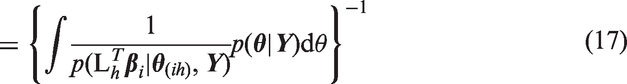
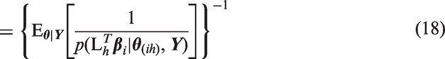
More generally, suppose we want to identify patients with outlying preferences on a combination of attribute variables. For example, in our application, urinary functioning and sexual functioning are represented by two attribute variables and thus two components 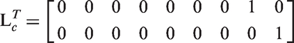$β_{i}$ . To do so, we can define an appropriate H × M indicator matrix $L_{c}$ in which each row selects one of the desired attribute variables. For example, to select the eighth and ninth elements of the attribute vector corresponding to short-term sexual issues and full sexual functioning, we can use

L_{c}^{T} = [000000010000000001]

Then the CPO for individual i and combination of attribute preferences c, which we could here denote as CPO-BVP (bivariate preference), is defined using equation (18)

{CPO-BVP}_{i}^{c} = {E_{θ | Y} [\frac{1}{p (L_{c}^{T} β_{i} | θ_{(ic)}, Y)}]} - 1

(19)

where

θ_{(ic)}

is the vector of model parameters

θ

minus

L_{c}^{T} β_{i}

. CPO-BVP can also be computed for other combinations of attributes, for example, full lifespan and others’ support. Drawing an MCMC sample of size G,

θ 1, \dots, θ G

from the full posterior density after the burn-in period allows us to obtain the following Monte Carlo approximations of CPO-BVP for individual i and list of attributes c

{CPO-BVP}_{i}^{c} \approx {\frac{1}{G} \sum_{g = 1}^{G} \frac{1}{p (L_{c}^{T} β_{i} | θ_{(ic)}^{g}, Y)}} - 1

(20)

We can also compute a more global outlier statistic for preferences. Identifying patients with outlying preferences on all attributes is a special case in which $L_{c}$ is the identity matrix of size H. We call this statistic ${CPO-MVP}_{i}$ .

6 Results

We fit the Bayesian hierarchical model of Section 3 to data from the 121 patients in the PROSPECT study. Dummy variables for three patient covariates were included in the model. These were: age (≥ 65 years vs. age < 65 years), race (black vs. white, other race vs. white), and partnered (vs. unpartnered). We chose a proper prior distribution⁴⁴ for $Σ - 1$ as $Wishart (9, \frac{1}{9} I_{9})$ , where $I_{9}$ is the 9 × 9 identity matrix, and we used Gibbs sampling implemented in JAGS⁴⁵ to obtain posterior samples. Three Markov chains were run, each with a burn-in of 20,000 iterations, followed by 100,000 iterations keeping every 10th draw of the chain. The final posterior sample consisted of 30,000 iterations (3 chains × 10,000 iterations).

The last two columns of Table 2 present the posterior means and standard deviations of the population mean preferences

μ

for the model without patient covariates. Attribute variables were considered significant if the posterior probability that the parameter is greater than zero was at least 95% or at most 5%. Preferences for all attributes were nonzero except for taking action. Sexual functioning appeared to be the most important attribute affecting health state preference followed by full lifespan, urinary functioning, no bowel issues, no cutting, and others’ support. For comparison, we also fit the model for best choices to our data (the first and second columns of results in Table 2). The comparison shows that, by using all available information (best and worst choices), we gain precision in our estimates (smaller posterior standard deviations). From Table 2, we see that our model for best–worst choices consistently provides more precise estimates than does the model for best choices, while providing similar results. Table 2 also presents the standard deviations of the attribute-specific random effects, which describe the between-subject variation. For both models, we can see a relatively high standard deviation of the random effect for full life, indicating substantial heterogeneity in preference between patients. Full sexual functioning also had high variance. In contrast, the random effects for taking action and others’ support have relatively low standard deviations indicating less heterogeneity.

Table 2.

Posterior means (standard deviations) of the components of the vector of population mean preferences $μ$ and the standard deviations of the random effects.

Attribute variable	Best choice		Best–worst choice
	Population mean	SD of random	Population Mean	SD of random
	μ_h	effect ε_ih	μ_h	effect ε_ih
Full life	2.67 (0.21)	1.79 (0.20)	2.20 (0.17)	1.68 (0.16)
No bowel issues	1.54 (0.15)	1.21 (0.15)	1.47 (0.13)	1.25 (0.12)
No cutting	0.88 (0.17)	1.33 (0.16)	0.79 (0.11)	0.97 (0.10)
Action	0.27 (0.12)	0.82 (0.10)	0.08 (0.08)	0.61 (0.06)
Others’ support	0.94 (0.14)	1.06 (0.13)	0.69 (0.10)	0.83 (0.08)
Short-term urinary issues	1.21 (0.17)	1.27 (0.17)	1.22 (0.13)	1.21 (0.12)
Full urinary functioning	1.98 (0.20)	1.48 (0.21)	1.83 (0.16)	1.53 (0.15)
Short-term sexual issues	1.99 (0.23)	1.97 (0.25)	1.55 (0.15)	1.47 (0.14)
Full sexual functioning	3.16 (0.29)	2.70 (0.31)	2.48 (0.21)	2.03 (0.19)

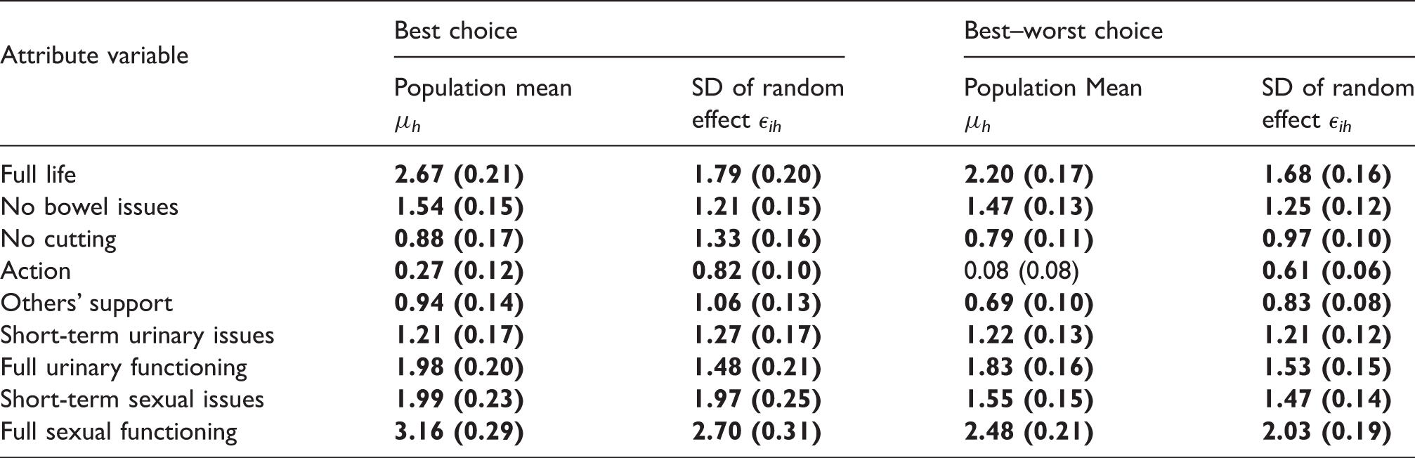
Note: Values in bold denote that the posterior probability that the parameter is greater than zero is greater than 95% or less than 5%.

Table 3 presents the correlation matrix of the random effects. The correlation between short-term urinary functioning and full urinary functioning is 0.84, as might be expected, since they measure the same attribute. We find the same relationship between short-term sexual functioning and full sexual functioning. No cutting is negatively correlated with each of the other attributes implying that patients who prefer no cutting place less value on all of the other attributes.

Table 3.

Posterior means (standard deviations) of the elements of the correlation matrix of the residual effect $ε_{i}$ for the model without patient covariates.

	Full life	No bowel issues	Short-term urinary issues	Full urinary functioning	Short-term sexual issues	Full sexual functioning	No cutting	Taking action	Others’ support
Full life	1
No bowel issues	0.15 (0.11)	1
Short-term urinary issues	0.28 (0.11)	0.29 (0.11)	1
Full urinary functioning	0.26 (0.11)	0.35 (0.11)	0.84 (0.04)	1
Short-term sexual issues	0.16 (0.11)	0.02 (0.12)	0.26 (0.11)	0.29 (0.11)	1
Full sexual functioning	0.19 (0.11)	−0.04 (0.11)	0.24 (0.11)	0.26 (0.11)	0.88 (0.03)	1
No cutting	−0.22 (0.12)	−0.09 (0.12)	−0.22 (0.12)	−0.24 (0.12)	−0.28 (0.11)	−0.24 (0.12)	1
Taking action	0.005 (0.13)	0.18 (0.13)	0.12 (0.13)	0.14 (0.13)	0.05 (0.13)	0.02 (0.14)	−0.11 (0.13)	1
Others support	−0.03 (0.13)	−0.09 (0.13)	−0.18 (0.12)	−0.15 (0.13)	−0.14 (0.12)	−0.21 (0.12)	−0.06 (0.13)	0.08 (0.13)	1

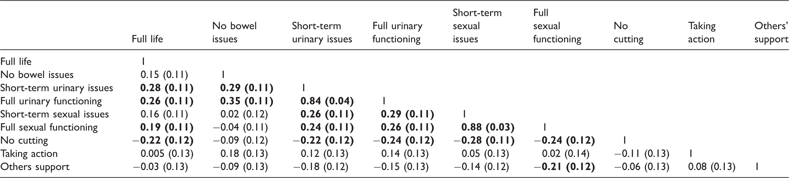
Note: Values in bold denote that the posterior probability that the parameter is greater than zero is greater than 95% or less than 5%.

Table 4 presents the posterior means and standard deviations of the regression coefficients

Γ

for the model including patient covariates and thus shows how preferences vary with age, race, and partnership status. The column labeled Intercept contains the posterior means and standard deviations corresponding to younger (<65 years old), white, and unpartnered patients. For this particular group, preferences for all attributes except taking action were nonzero. Older men (≥ 65 years old) appeared to favor full lifespan and urinary functioning more than younger men. For older men, each of these attributes was associated with approximately a 0.7 and 0.6 (respectively) higher estimated patient preference score than younger men. Differences in preferences were also found by partnership status. Partnered men favored full lifespan more than unpartnered men by 0.98 points.

Table 4.

Posterior means (standard deviations) of the elements of the matrix of regression coefficients $Γ$ and the standard deviations of the random effects.

Attribute variable	Patient-specific covariate
	Intercept	≥ 65 years	Black	Other race	Has partner	SD of residual
		(vs. < 65 years)	(vs. White)	(vs. White)	(vs. Does not)	effect εi _h
Full life	1.35 (0.35)	0.72 (0.32)	−0.14 (0.34)	−0.12 (0.39)	0.98 (0.33)	1.70 (0.17)
No bowel issues	1.36 (0.29)	0.11 (0.26)	0.38 (0.29)	0.23 (0.32)	−0.12 (0.27)	1.31 (0.12)
No cutting	0.66 (0.25)	0.06 (0.22)	0.03 (0.24)	0.21 (0.28)	0.10 (0.23)	1.01 (0.10)
Taking action	0.26 (0.18)	−0.12 (0.15)	−0.01 (0.17)	−0.17 (0.20)	−0.12 (0.16)	0.63 (0.06)
Others’ support	0.76 (0.22)	−0.35 (0.19)	−0.12 (0.21)	−0.16 (0.24)	0.28 (0.20)	0.83 (0.09)
Short-term urinary issues	1.14 (0.27)	0.54 (0.24)	0.03 (0.27)	−0.39 (0.30)	−0.11 (0.25)	1.22 (0.12)
Full urinary functioning	1.67 (0.34)	0.60 (0.31)	0.14 (0.33)	−0.29 (0.37)	−0.09 (0.32)	1.55 (0.16)
Short-term sexual issues	1.64 (0.30)	−0.01 (0.28)	0.004 (0.30)	−0.72 (0.33)	0.18 (0.28)	1.48 (0.15)
Full sexual functioning	2.27 (0.40)	−0.05 (0.38)	0.13 (0.40)	−0.24 (0.45)	0.45 (0.39)	2.12 (0.20)

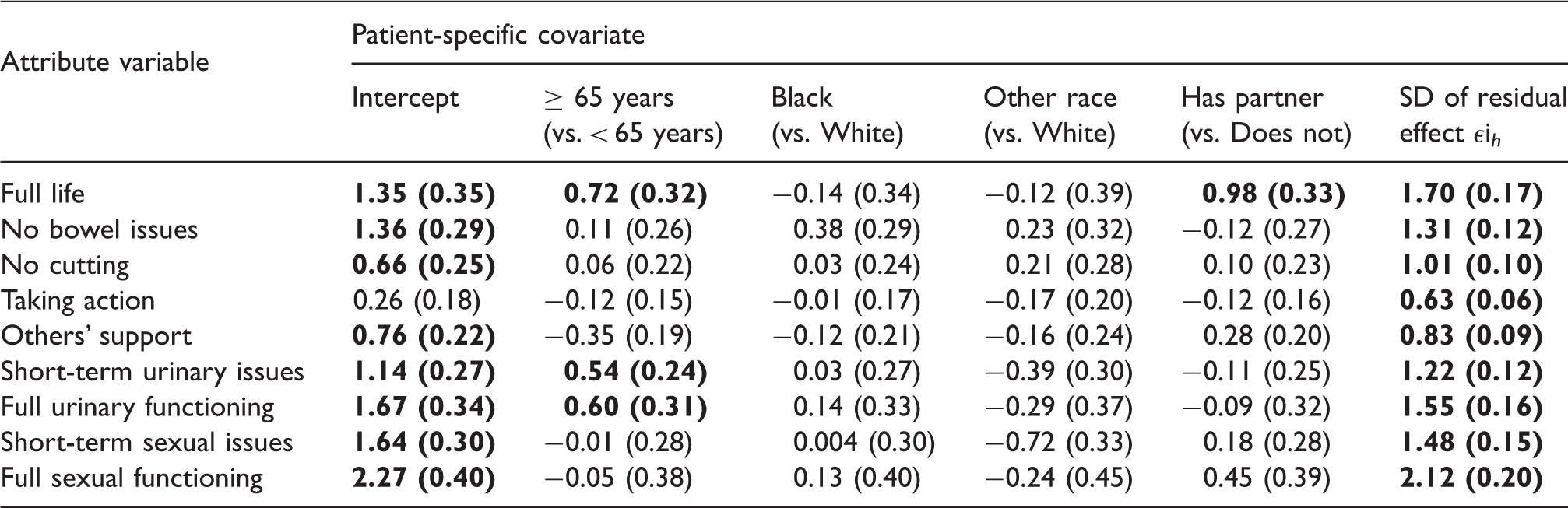
Note: Values in bold denote that the posterior probability that the parameter is greater than zero is greater than 95% or less than 5%.

Figure 2 presents the posterior mean average relative importance scores for each health state attribute for the population and the posterior mean relative importance scores for 14 sample patients. To select the 14 patients in Figure 2, patients were sorted by decreasing the relative importance score on full lifespan and every 10th ranked patient was selected. This figure shows the heterogeneity of preferences for health state attributes in the sample. Greater heterogeneity in preference for full lifespan and lower heterogeneity in preference for taking action were apparent.

Figure 2.

Posterior mean relative attribute importance scores for each health state attribute for 14 men and for the population.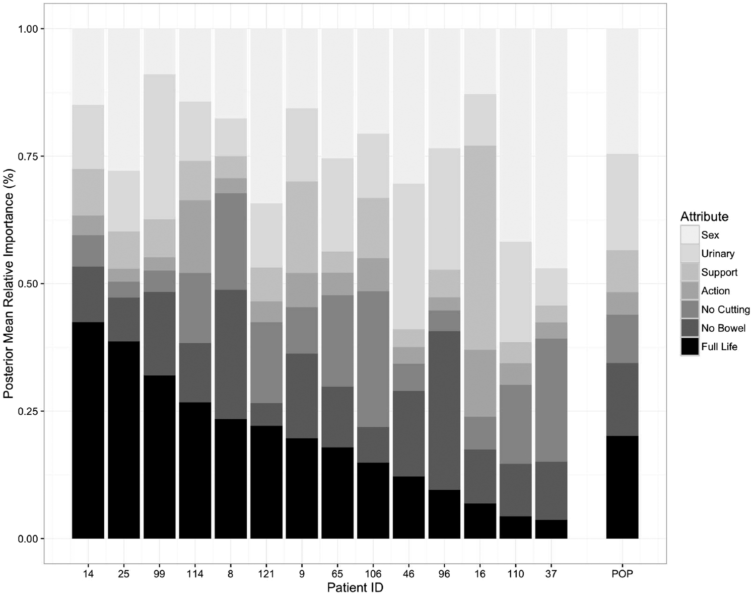

Table 5 presents the posterior mean relative importance scores for each health state attribute for the population and for three sample patients. In general, the standard deviations of the relative importance scores are small relative to the posterior means, suggesting that the posterior means provide a reliable ranking of attributes by relative importance. At a population level, sexual functioning, urinary functioning, and full lifespan appear to be the three most important attribute variables, whereas taking action appears to be the least important. Patient 115 clearly placed the highest importance on full lifespan, a moderate importance on bowel issues, and a low importance on all other attributes. Patient 13 placed the highest importance on urinary functioning and sexual functioning. Patient 108 has posterior mean estimates similar to those of the population.

Table 5.

Posterior mean (standard deviation) of relative attribute importance scores for three men and for the population.

Attribute	Patient 115	Patient 13	Patient 108	Population
Full life	0.41 (0.05)	0.07 (0.04)	0.22 (0.05)	0.201 (0.005)
No bowel issues	0.22 (0.03)	0.09 (0.04)	0.11 (0.05)	0.143 (0.004)
No cutting	0.07 (0.03)	0.07 (0.04)	0.07 (0.04)	0.094 (0.004)
Taking action	0.02 (0.02)	0.07 (0.03)	0.04 (0.03)	0.044 (0.004)
Others’ support	0.07 (0.03)	0.04 (0.03)	0.07 (0.05)	0.082 (0.004)
Urinary functioning	0.10 (0.04)	0.31 (0.05)	0.16 (0.06)	0.189 (0.006)
Sexual functioning	0.12 (0.04)	0.35 (0.06)	0.34 (0.07)	0.245 (0.006)

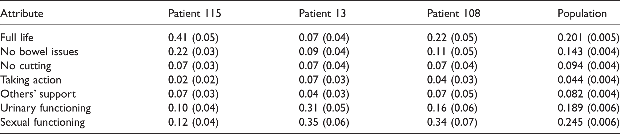
Figure 3 presents boxplots of CPO-MVP values for the set of all attributes, CPO-UVP values for specific attributes, and CPO-BVP values for the two bivariate combinations of attributes for urinary and sexual functioning for the 121 patients. A negative log-transformation was applied to the CPOs to better visualize small values. High values of negative log-transformed CPOs indicate possible outliers (low CPO). Patients 15, 83, and 17 are multivariate outliers on the set of all attribute variables by CPO-MVP. Patient 83 is also outlying on the bivariate CPO for urinary functioning and the bivariate CPO for sexual functioning. Patient 15 had highest negative log-transformed CPO-UVP values on others’ support. Patient 17 is an example of a multivariate outlier that cannot be detected by looking at outliers on specific health state attributes, while patient 54 is an example of a patient with outlying preferences on a single attribute who is not a multivariate outlier.

Figure 3.

Plot of the −log(CPO-MVP)s on all health state attributes, the −log(CPO-UVP)s for specific attributes, and the −log(CPO-BVP)s for the bivariate combinations of attributes for urinary and sexual functioning for 121 patients. Patients with values of the outlier statistic in the upper 2.5th percentile are labeled with ID numbers.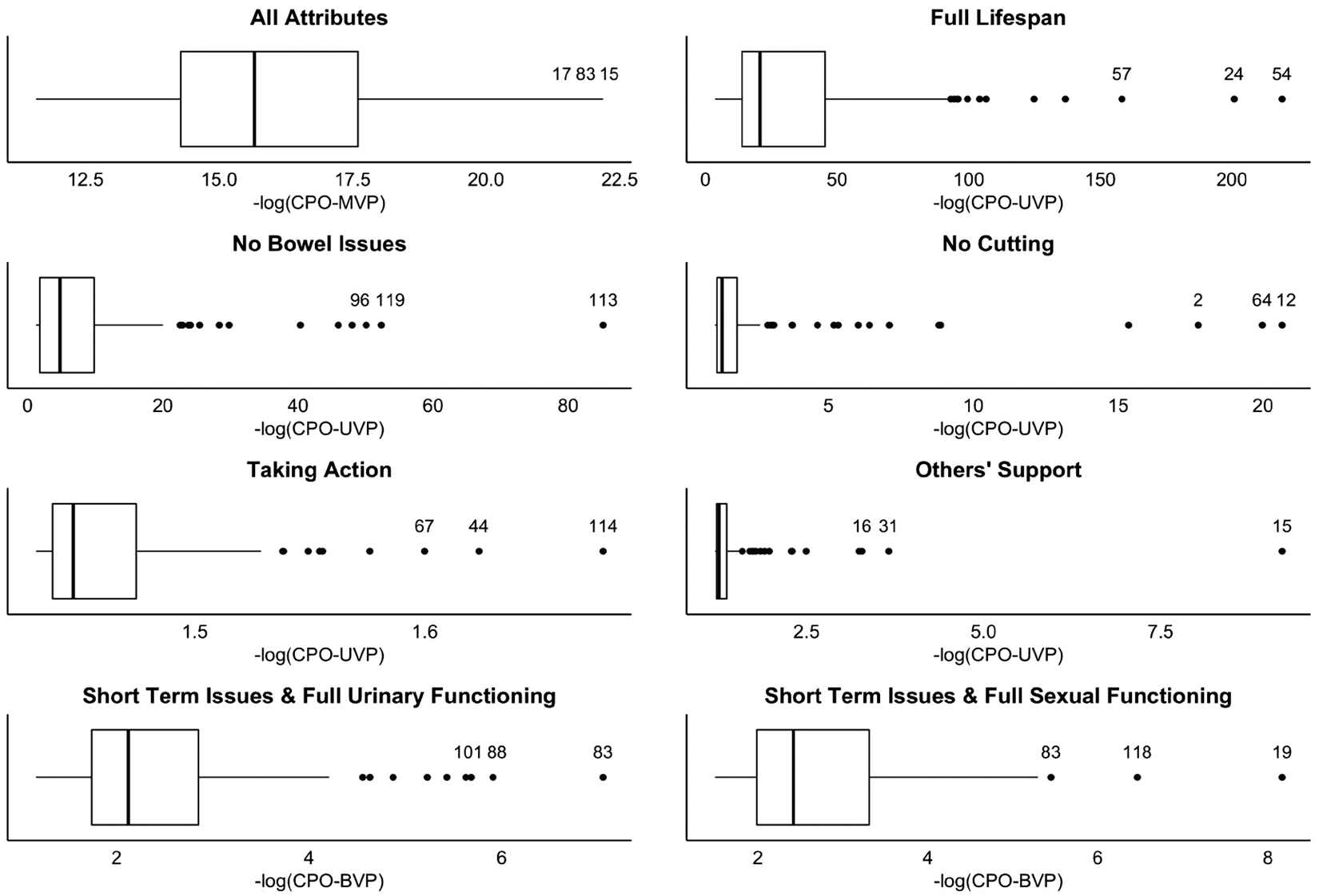

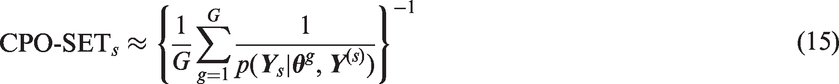
Figure 4 presents the time series of the negative log CPO values for choice sets presented to eight patients. DCEs require patients to evaluate a number of different choice sets and some patients may undergo a learning effect where accuracy in responses improves with time. Conversely, some patients may become fatigued and accuracy of their responses may degrade as the number of questions increases.^46,47 By examining these time series, we can gain insight as to an individual’s performance on discrete choice tasks, and observe possible learning effects or fatigue effects, and whether they made choices on specific sets that were inconsistent with their preferences. High values of negative log-transformed CPO indicate possible outlying choice sets. Patient 115 is an example of a patient with consistent responses and no outliers. In contrast, patient 52 shows highly variable responses, which might indicate more difficulty with the choice tasks. Patient 10 has an outlier on the first choice set, which may indicate a cognitive error early in the exercise. Patient 109 shows an upward trend suggesting a possible fatigue effect and an especially inconsistent choice on the second to last choice set. For patient 74, we observe a downward trend suggesting a learning effect where patient performance on choice tasks improves over time.

Figure 4.

Plot of the −log(CPO-SET)s calculated for each choice set presented to eight patients.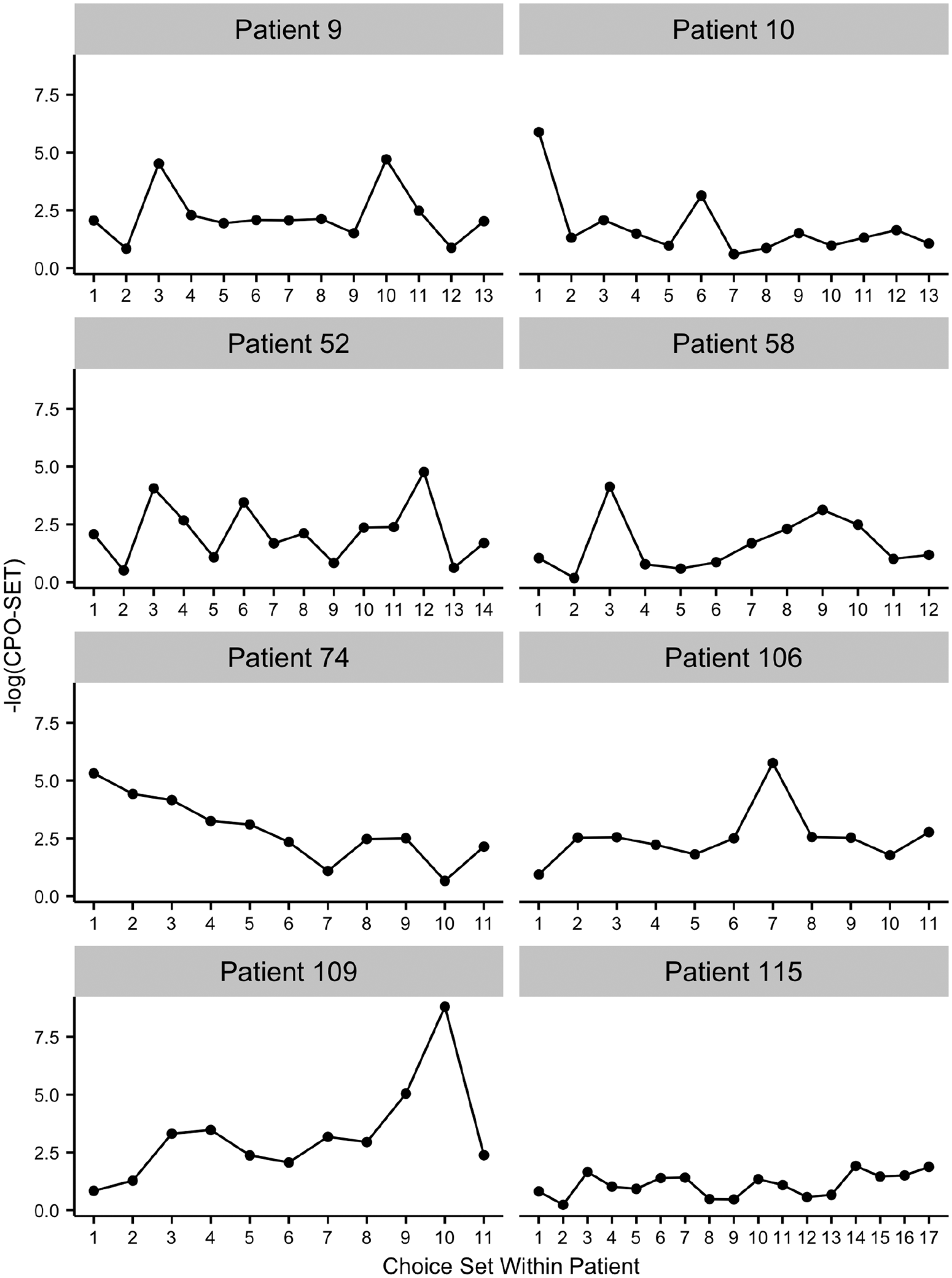

We conducted sensitivity analyses on the prior assumptions $Wishart (w, W)$ for the random effects precision matrix $Σ - 1$ by comparing the posterior results over variations of the prior. With degrees of freedom parameter w and scale matrix W , we explored the following Wishart specifications: w = 9 and $W = \frac{1}{9} I$ , w = 9 and $W = \frac{1}{18} I$ , w = 18 and $W = \frac{1}{9} I$ , w = 18 and $W = \frac{1}{18} I$ . There was little change in the posterior estimates for the elements of the correlation matrix or the population preference parameters with different specifications, indicating that the results were fairly robust to changes in the hyperprior specifications.

7 Discussion

We developed a Bayesian hierarchical model for best–worst discrete choice data that accounts for incomplete rankings and includes patient covariates. The model can handle sparse data and is particularly useful when discrete choice experiments involve relatively few choice sets per patient. Although our application had choice sets of size 4, the model can be applied to studies with larger choice sets.

The main goal of our discrete choice experiment was to identify health state attributes that are most important to individual patients to guide that individual’s treatment; thus, we presented Bayesian versions of a commonly used measure of relative attribute importance. The estimates of relative attribute importance include posterior standard deviations that reflect uncertainty; in the literature, many studies only provide point estimates which may give false confidence about how the patient ranks the attributes. Our method for computing relative attribute importance is not specific to best–worst DCE and can be applied to other DCE designs. The concept of relative attribute importance is akin to the concept of variable importance in regression and prediction modeling. We have not explored other possible measures of variable importance that might be applied to DCE. The measurement of relative variable importance is an active area of research.^48–53

We have shown how the conditional predictive ordinate can be adapted to identify outlying choice sets and outlying patients with unusual preferences in discrete choice data. Our CPO for identifying preference outliers finds outliers in the random effects. Random effects are a common feature of Bayesian models, and this new application of the CPO could have broader application in Bayesian modeling. The method is quite flexible and general, and can even identify outliers on sets of multiple random effects. We have shown how the method can be applied to identify outliers on categorical attributes modeled using two coefficients. The CPO for identifying outlying choice sets utilizes a vector outcome and is also an important extension of the CPO that could be used in other applications.

Our application includes two attributes, sexual functioning and urinary functioning, whose attribute levels are naturally ordered; the levels of sexual functioning are none, decreased and full, and the levels of urinary functioning are long-term issues, short-term issues, and full functioning. One approach to estimate the corresponding coefficients would be to impose order constraints, such that the coefficient for decreased functioning must be less than or equal to the coefficient for full functioning. This could be accomplished by specifying a truncated multivariate prior density on the vector of random effects and the vector of population effects.⁴⁰ However, we obtained satisfactory results without imposing such constraints.

Experimental design for DCEs is an area of active research^54,55; however, there is little consensus on the optimal design of choice experiments, including how to generate choice sets.^56,57 A recent report described alternative approaches to experimental design for DCEs,⁵⁴ but did not recommend any specific approach as best practice. The choice of alternatives for each choice set and the choice sets presented to each patient are important with regard to statistical efficiency. Random selection of profiles to choice sets may result in choice sets for which little information is gained on relative preferences because the attributes are not varied sufficiently. In addition, increasing the number of choice sets presented to patients can increase cognitive burden, jeopardizing the quality of patient responses. When creating a DCE, a trade-off is made between maximizing statistical efficiency and maximizing respondent efficiency (measurement error related to the quality of responses). A direction for future research would be to formally evaluate the impact of the experimental design on estimation of preferences.

Our DCE uses factors with different numbers of levels. Studies have shown that there is a positive association between the number of attribute levels and attribute importance scores.^58,59 Designing a study with the same number of attribute levels for each attribute may not be acceptable for some applications. In our study, all of our attributes have either two or three levels. We think it reasonable that a priori important variables, such as urinary and sexual functioning, would be modeled using more levels. We fit the model after collapsing the two highest categories of urinary functioning and sexual functioning into a single category and obtained similar posterior means. Hence, we surmise that the different numbers of levels did not appreciably affect our results.

The development of best–worst discrete choice designs reduces patient burden compared to full rankings while posing new statistical challenges. By accounting for missing ranking information, patient covariates, and the sparse nature of the individual-level data in a Bayesian framework, our model extends current methods and provides individual-level preference estimates. Our CPO measures provide some of the first diagnostic techniques for discrete choice models. Our model coupled with our measures of relative importance and outlyingness, provides practical methodology for discrete choice modeling applications, in which parameter estimation at the individual-level is desirable, but observed data at the individual-level are limited.

Footnotes

Acknowledgements

We mourn the passing of our esteemed colleague Ely Dahan, who passed away before this work could be published, and are deeply grateful for his contributions.

Declaration of conflicting interests

The author(s) declared no potential conflicts of interest with respect to the research, authorship, and/or publication of this article.

Funding

The author(s) disclosed receipt of the following financial support for the research, authorship, and/or publication of this article: Saigal, Dahan, and Crespi were supported by grant from the National Cancer Institute (grant no. 5R01CA134997-02). Crespi was also supported by NIH/NCI P30 CA16042. The content is solely the responsibility of the authors and does not necessarily represent the official views of the National Cancer Institute or the National Institutes of Health.

Appendix 1

References

Lancsar

Louviere

Donaldson

et al.

Best worst discrete choice experiments in health: methods and application. Social Sci Med 2013; 76: 74–82.

DeBekker-Grob

Ryan

Gerard

. Discrete choice experiments in health economics: a review of the literature. Health Econom 2012; 21: 145–172.

Ryan

Gerard

Amaya-Amaya

. Using discrete choice experiments to value health and healthcare, 1st ed. Dordrecht, The Netherlands: Springer, 2008.

Lancsar

Louviere

. Estimating individual level discrete choice models and welfare measures using best worst choice experiments and sequential best worst MNL. In: CenSoC Working Paper Series. 08–003.

Louviere

Street

Burgess

et al.

Modelling the choices of individual decision-makers by combining efficient choice experiment designs with extra preference information. J Choice Model 2008; 1: 128–163.

Allenby G, Rossi P and McCulloch R. Hierarchical Bayes models: a practitioners guide, SSRN Working Paper, https://papers.ssrn.com/sol3/papers.cfm?abstract_id=655541 (2005, accessed 2 February 2017).

Rao

Developments in conjoint analysis. In: Wierenga

(ed). Handbook of marketing decision models, Boston, MA: Springer, 2008, pp. 23–53.

McFadden

Conditional logit analysis of qualitative choice behavior. In: Zarembka

(ed). Frontiers in Economics, New York, NY: Wiley, 1974, pp. 105–142.

Allison

Christakis

. Logit models for sets of ranked items. Sociol Methodol 1994; 24: 199–228.

10.

Revelt

Train

. Mixed logit with repeated choices: households’ choices of appliance efficiency level. Rev Econom Stat 1998; 53: 647–657.

11.

McFadden

Train

. Mixed MNL models for discrete response. J Appl Econom 2000; 5: 447–470.

12.

Hernandez-Alava

Brazier

Rowen

et al.

Common scale valuations across difference preference-based measures: estimation using rank data. Med Decis Making 2013; 6: 839–852.

13.

Crabbe

Vandebroek

. Improving the efficiency of individualized designs for the mixed logit choice model by including covariates. Comput Stat Data Anal 2011; 56: 2059–2072.

14.

Orme B and Howell J. Application of covariates within Sawtooth Software’s CBC/HB program: theory and practical example. In: Sawtooth software conference papers. Sequoia, WA: Sawtooth Software, http://www.sawtoothsoftware.com/download/techpap/HBCovariates.pdf (2009, accessed 1 February 2017).

15.

Greene

Hensher

Rose

. Accounting for heterogeneity in the variance of unobserved effects in mixed logit models. Transport Res Part B: Methodol 2006; 40: 75–92.

16.

Paul

Green

. Conjoint analysis in consumer research: Issues and outlook. J Consumer Res 1978; 5: 103–123.

17.

Halbrendt

Wang

Fraiz

et al.

Marketing problems and opportunities in Mid-Atlantic seafood retailing. Am J Agri Econom 1995; 77: 1313–1318.

18.

Orme

. Getting started with conjoint analysis: strategies for product design and pricing research, 2nd ed. Madison, WS: Research Publishers LLC, 2010, pp. 29–37.

19.

Dowsey

Scott

Nelson

et al.

Using discrete choice experiments as a decision aid in total knee arthroplasty: study protocol for a randomised controlled trial. Trials 2016; 17: 1–10.

20.

Kruk

Riley

Palma

et al.

How can the health system retain women in HIV treatment for a lifetime? A discrete choice experiment in Ethiopia and Mozambique. PLoS ONE 2016; 11: 1–14.

21.

van Dijk

Groothuis-Oudshoorn

CGM

Marshall

et al.

An empirical comparison of discrete choice experiment and best–worst scaling to estimate stakeholders

:

risk tolerance for hip replacement surgery. Value in Health 2016; 19: 316–322.

22.

Train K. A comparison of hierarchical Bayes and maximum simulated likelihood for mixed logit. Working Paper no. E00-278, University of California, Berkeley 2001.

23.

Train

. Discrete choice methods with simulation, 2nd ed. New York, NY: Cambridge University Press, 2009.

24.

Campbell D and Hess S. Outlying sensitivities in discrete choice data: consequences and remedies. Working paper, http://www.webmeets.com/files/papers/WCERE/2010/1194/world_congress.pdf (2010, accessed 1 February 2017).

25.

Farrel

Groshen

MacGibbon

et al.

Outlier detection for a hierarchical Bayes model in a study of hospital variation in surgical procedures. Stat Meth Med Res 2012; 19: 601–619.

26.

Chaloner

Brant

. A Bayesian approach to outlier detection and residual analysis. Biometrika 1988; 75: 651–659.

27.

Chaloner

. Bayesian residual analysis in the presence of censoring. Biometrika 1991; 78: 637–644.

28.

Chaloner

Residual analysis and outliers in Bayesian hierarchical models. In: Smith

Freeman

(eds). Aspects of uncertainty, Chichester, UK: Wiley, 1994, pp. 149–157.

29.

Box

. Discussion of sampling and Bayes inference in scientific modelling and robustness. J Royal Stat Soc: Series A 1980; 143: 416–417.

30.

Geisser

. Influential observations, diagnostics and discovery tests. J Appl Stat 1987; 14: 133–142.

31.

Geisser

. Predictive discordancy tests for exponential observations. Can J Stat 1989; 17: 19–26.

32.

Geisser

. Predictive inference, New York, NY, Taylor & Francis: Chapman & Hall/CRC Monographs on Statistics & Applied Probability, 1993.

33.

Dey

Chen

Chang

. Bayesian approach for nonlinear random effects models. Biometrics 1997; 53: 1239–1252.

34.

Pettit

. The conditional predictive ordinate for the normal distribution. J Royal Stat Soc Ser B 1990; 52: 175–184.

35.

Saigal C and Dahan E. Voice of the patient. In: Proceedings of the Sawtooth software conference, Orlando, FL, 21–23 March 2012. Sawtooth Software, Inc., pp.153–164.

36.

Hauber

Gonzalez

Groothuis-Oudshoorn

et al.

Statistical methods for the analysis of discrete choice experiments: a report of the ISPOR conjoint analysis good research practices task force. Value Health 2016; 19: 300–315.

37.

Bergland O. Estimation of stated preferences from incomplete ranking. In: Discussion Papers. Number D-05 in Discussion Paper Series, Department of Economics and Social Sciences, Agricultural University of Norway.

38.

Chapman

Staelin

. Exploiting rank ordered choice set data within the stochastic utility model. J Market Res 1982; 19: 288–301.

39.

Soofi

Retzer

Yasai-Ardekani

. A framework for measuring the importance of variables with applications to management research and decision models. Decis Sci 2000; 31: 595–625.

40.

Gelfand

Smith

Lee

. Bayesian analysis of constrained parameter and truncated data problems using Gibbs samplings. J Am Stat Assoc 1992; 87: 523–532.

41.

Gelfand

Model determination using sampling-based methods. In: Gilks

Richardson

Spiegelhalter

(eds). Markov Chain Monte Carlo in practice, Chapter 9, Boca Raton, FL: Chapman & Hall, 1996, pp. 145–161.

42.

Weiss

. Pediatric pain, predictive inference, and sensitivity analysis. Eval Rev 1994; 18: 651–677.

43.

Weiss

. An approach to Bayesian sensitivity analysis. J Royal Stat Soc Ser B (Methodological) 1996; 58: 739–750.

44.

Gelman

. Prior distributions for variance parameters in hierarchical models. Bayesian Anal 2006; 1: 515–533.

45.

Plummer M. JAGS: a program for analysis of Bayesian graphical models using Gibbs sampling. In: Proceedings of the 3rd International Workshop on Distributed Statistical Computing, Technische Universität Wien, Vienna, Austria, 20–22 March 2003.

46.

Bradlow

Weiss

Cho

. Bayesian identification of outliers in computerized adaptive tests. J Am Stat Assoc 1998; 93: 910–919.

47.

Hauser

Rao

. Conjoint analysis, related modeling and applications. Market Res Model: Progr Prospect Int Ser Quantitative Market 2002; 14: 141–168.

48.

Kruskal

Majors

. Concepts of relative importance in recent scientific literature. Am Stat 1989; 43: 2–6.

49.

Retzer

Soofi

Soyer

. Information importance of predictors: concept, measures, Bayesian inference, and applications. Comput Stat Data Anal 2009; 53: 2363–2377.

50.

Johnson

Lebreton

. History and use of relative importance indices in organizational research. Organiz Res Meth 2004; 7: 238–257.

51.

. A review of statistical methods for determination of relative importance of correlated predictors and identification of drivers of consumer liking. J Sensory Stud 2012; 27(2): 87–101.

52.

Grömping

. Variable importance in regression models. Wiley Interdiscipl Rev: Computat Stat 2015; 7: 137–152.

53.

Harris

Burch

. Measuring relative importance of sources of variation without using variance. Am Stat 2005; 59: 217–222.

54.

Johnson

Lancsar

Marshall

et al.

Constructing experimental designs for discrete-choice experiments: report of the ISPOR conjoint analysis experimental design good research practices task force. Value Health 2013; 16: 3–13.

55.

Jaynes

Wong

. Using blocked fractional factorial designs to construct discrete choice experiments for healthcare studies. Stat Med 2016; 35: 2543–2560.

56.

Lusk

Norwood

. Effect of experimental design on choice-based conjoint valuation estimates. Am J Agri Econom 2005; 87: 771–785.

57.

Louviere

Pihlens

Carson

. Design of discrete choice experiments: A discussion of issues that matter in future applied research. J Choice Model 2011; 4: 1–8.

58.

Wittink

Krishnamurthi

Nutter

. Comparing derived importance weights across attributes. J Consum Res 1982; 8: 471–474.

59.

Wittink

Krishnamurthi

Reibstein

. The effect of differences in the number of attribute levels on conjoint results. Market Lett 1990; 1: 113–123.