Bayesian quantile regression-based partially linear mixed-effects joint models for longitudinal data with multiple features

Abstract

In longitudinal AIDS studies, it is of interest to investigate the relationship between HIV viral load and CD4 cell counts, as well as the complicated time effect. Most of common models to analyze such complex longitudinal data are based on mean-regression, which fails to provide efficient estimates due to outliers and/or heavy tails. Quantile regression-based partially linear mixed-effects models, a special case of semiparametric models enjoying benefits of both parametric and nonparametric models, have the flexibility to monitor the viral dynamics nonparametrically and detect the varying CD4 effects parametrically at different quantiles of viral load. Meanwhile, it is critical to consider various data features of repeated measurements, including left-censoring due to a limit of detection, covariate measurement error, and asymmetric distribution. In this research, we first establish a Bayesian joint models that accounts for all these data features simultaneously in the framework of quantile regression-based partially linear mixed-effects models. The proposed models are applied to analyze the Multicenter AIDS Cohort Study (MACS) data. Simulation studies are also conducted to assess the performance of the proposed methods under different scenarios.

Keywords

Asymmetric Laplace distribution Bayesian inference longitudinal quantile regression partially linear mixed-effects joint models limit of detection covariate measurement errors

1 Introduction

In HIV/AIDS studies, as important biomarkers of AIDS pathogenesis, severity of viral infection, and disease progression, repeatedly measured viral load (the number of copies of HIV-1 RNA per milliliter plasma), and CD4 cell counts have been widely studied.^1–5 The relationship between them is also of interest, which may help clinicians better understand AIDS pathophysiology, and evaluate treatment effect. Although the negative relationship is widely accepted, it just measures a very general and rough mean relationship. In fact, the effect of CD4 counts is more important among subjects with higher viral load, who are at higher risk. Thus, it is desirable to develop new models to give this relationship a full scan and have a comprehensive understanding.

In statistics, mixed-effects models are becoming increasingly popular in longitudinal data analysis. However, the majority of longitudinal modeling methods are based on mean regression to concentrate only on the average effect of covariate and the mean trajectory of longitudinal outcome. Furthermore, if obvious outliers and/or heavy tails exist, mean regression may lead to inappropriate parameter estimates. For example, in the Multicenter AIDS Cohort Study (MACS)⁶ (refer to Section 2.1 for the details of this study and data description), the viral load measurements are highly skewed with heavy tails, even after log₁₀ transformation (Figure 1(a)). When heavy tails and outliers exist, it is well known that median regression, a special case of Quantile regression (QR), is more robust than the traditional mean regression. QR introduced by Koenker and Bassett⁷ has been rapidly expended in economics, social sciences, engineering and biomedical research.^8–12 Longitudinal QR models have been proposed from both frequentist’s^13–19 and Bayesian view,^20–25 respectively.

Figure 1.

Histogram (left panel) of viral load (response) in ${log}_{10}$ scale and standardized CD4 cell counts for 435 subjects with seroconversion from MACS data. Profiles (right panel) of viral load (response) in ${log}_{10}$ scale and CD4 cell count (covariate) for five representative patients. (a) Histogram of log10(RNA), (b) Profiles of log10(RNA), (c) Histogram of standardized CD4, (d) Profiles of standardized CD4 cell counts.

Parametric regression methods for longitudinal data have been well developed in the last 30 years.^26,27 A major limitation of these methods is that when the relationship of the longitudinal outcome to covariates is assumed fully parametric, they have suffered from the inflexibility and possible misspecification in modeling complicated longitudinal data. For example, in MACS data, as shown in Figure 1(b), the longitudinal trajectory of viral load for each patient is quite irregular. Thus, to weaken model assumption, it is more appropriate to model such varying trajectories by a flexible nonparametric function of time. However, if we consider nonparametric functions for all covariates, it may bring the problem known as “curse of dimensionality”. Also, the parametric relationship between viral load and CD4 cell counts is of interest. With this consideration, we adopt a partially linear mixed-effects model (PLMM) which has received much attention in statistics.^28–31 In this study, the PLMM serves as an intermediate class of models with good robustness by nonparametric treatment on time covariate and a more precise estimation on the parametric effect of CD4 counts.

However, in practice, certain inherent data features make the complicated longitudinal data far from ideal. The analysis of such “imperfect” data poses statistical challenges. First, the small concentration cannot be precisely measured when the actual quantity is below the limit of detection (LOD) (see Figure 1(b)), due to the low sensitivity of current technology. In the MACS data set that we have used in this study, about 26% observations of viral load fell below the LOD (50 copies/ml), which may result in significant biases.^23,32 In statistical analyses, these values called left-censored values are often substituted with a constant, such as half the LOD, the LOD divided by $\sqrt{2}$ , or even zero. Compared to the imputation method, a Tobit model is used to treat the left-censoring issue more precisely.^32,33 Second, covariates in the longitudinal data may suffer from measurement errors. For example, in AIDS research, CD4 cell counts are often measured with substantial errors, and ignoring this phenomenon may lead to biased inference.^1–3 Third, skewness is commonly observed in AIDS studies, such as CD4 cell counts (Figure 1(c)), but most of the statistical models assume that the error terms follow normal distribution because of the computational convenience.^1–3,5 Although the findings from those models still dominate the applications, it is well known that the misspecified normal assumption could produce misleading results and lack the robustness.^4,34,35 Transformation is one of the solutions for skewness, like the transform-both-sides (TBS) approach,³⁶ but the viral load and CD4 counts in MACS data are still skew-distributed after transformation or standardization. Recently, models with skew-elliptical (SE) distributions, which include skew-normal (SN) and skew-t (ST) distributions (see Appendix 1.1 in detail), have received much attention, while the “normality” assumption is violated. We adopt the SN and ST distributions introduced by Sahu et al.³⁷ for the covariate measurement error process.

To the best of our knowledge, little work has been conducted on modeling longitudinal data via PLMM under QR-based framework and simultaneously accounting for LOD and covariate measurement error. The main purpose of this paper is to examine the heterogeneous relationship between viral load and CD4 cell counts, and the longitudinal trajectory at different quantiles of viral load, considering LOD and mismeasured covariate with skewness simultaneously. Thus, we first propose QR-based partially linear mixed-effects joint models (QR-PLMJM) which consist of (i) QR-based PLMM with the asymmetric Laplace distribution (ALD)³⁸ (see Appendix 1.2 in detail) considering left censoring due to LOD, and (ii) linear mixed-effects (LME) models with skewed distributions for covariate process. Since statistical inference becomes dramatically complicated when these issues exist, a Bayesian inferential approach is applied to estimate parameters of the joint models.

The rest of the paper is organized as follows. In Section 2, we describe the data set that motivated this study and propose a specific QR-PLMJM. Section 3 presents the related Bayesian inferential method. In Section 4, we apply the proposed QR-PLMJM to the data set described in Section 2 and report the results. Section 5 conducts simulation studies to evaluate the performance of the proposed models and method. Finally, general discussion and conclusion are presented in Section 6.

2 Quantile regression-based partially linear mixed-effects joint models

2.1 Motivating data set

The data set that motivated this study is from the MACS, which recruited men who reported having had sex with men at one of the four metropolitan areas in the USA (Baltimore, Chicago, Pittsburgh, and Los Angeles) during three recruitment periods (from April 1984 through March 1985, from April 1987 through September 1991, and from October 2001 through August 2003). Participants in the MACS had baseline and semi-annual follow-up visits for a detailed interview, physical examination, neuropsychological testing, and collection of blood for laboratory testing. The subset of MACS participants who seroconvert with HIV are of interest, since they are followed up from the time when they first develop antibodies to HIV. Due to the particular interest of the relationship between two important biomarkers: HIV viral load and CD4 cell counts, our data analysis is based on 435 patients with recorded HIV seroconversion, and at least three measures of HIV viral load. Of the 435 subjects with a total of 6437 observations, 1680 (26%) viral load data fell below the LOD. The details about the recruitment and characteristics of the MACS cohort have been reported elsewhere.⁶

Additionally, certain variables were transformed or imputed to benefit our analysis process. For example, the viral load was taken a ${log}_{10}$ transformation, and CD4 cell counts were standardized (i.e. each CD4 count is subtracted by mean 556.25 and divided by standard deviation 325.01) in order to stabilize the variation of the measurements and to accelerate the convergence of estimation algorithm. One limitation of the public MACS data was that the time of visit for each patient was only recorded at the year level. To account for the limitation, according to the study by Chen et al.,³⁹ we imputed the visit time according to the following criteria: (1) if a participant visited twice in year X, the time of the first visit was recorded as X, and the second visit was computed as $X + 0.5$ ; (2) for a subject with three visits, time was imputed as X, $X + 0.33$ , and $X + 0.67$ , respectively. Also, in order to avoid unstable estimates with extreme value, the original time t was rescaled to ensure that the time scale is between 0 and 1.

2.2 CD4 covariate measurement error model with ST distribution

In AIDS studies, CD4 cell counts are usually measured with substantial errors, and highly skewed. Various covariate mixed-effects models were discussed in the literature, but most of them assume normal distribution for error term which may lack the robustness against departures from normality in practice.^1,2,40 In order to relax the normality assumption and make a robust inference, we assume the models with SE distributions, including SN and ST distributions. The ST distribution, the more general one, is approximate to the SN distribution when its degrees of freedom increase to infinity. This section briefly discusses CD4 covariate measurement error models with an ST distribution. Thus, in the presence of covariate measurement errors, we consider the following LME model to quantify the covariate process.

\begin{matrix} z_{ij} = u_{ij}^{T} α + v_{ij}^{T} a_{i} + ε_{ij} (\equiv z_{ij}^{*} + ε_{ij}), \\ ε_{i} \sim^{iid} {ST}_{n_{i}, ν} (- J (ν) δ 1_{n_{i}}, σ_{1}^{2} I_{n_{i}}, δ I_{n_{i}}) \end{matrix}

(1)

where

z_{i} = (z_{i 1}, \dots, z_{{in}_{i}})^{T}

with z_ij being the observed CD4 covariate value for individual i at time t_ij,

z_{i}^{*} = (z_{i 1}^{*}, \dots, z_{{in}_{i}}^{*})^{T}

and

z_{ij}^{*} = u_{ij}^{T} α + v_{ij}^{T} a_{i}

may be viewed as the true (but unobservable) covariate value at time t_ij,

u_{ij}

and

v_{ij}

are

l \times 1

design vectors,

α = (α_{1}, \dots, α_{l})^{T}

and

a_{i} = (a_{i 1}, \dots, a_{il})^{T}

are unknown population (fixed-effects) and individual-specific (random-effects) parameter vectors, respectively;

ε_{i} = (ε_{i 1}, \dots, ε_{{in}_{i}})^{T}

follows a multivariate ST distribution with unknown variance parameter

σ_{1}^{2}

, skewness parameter δ and degrees of freedom ν, where the location parameter is set as

- J (ν) δ 1_{n_{i}}

with

- J (ν) = (ν / π)^{1 / 2} [Γ ((ν - 1) / 2) / Γ (ν / 2)]

in order to have a zero-mean vector for error term and

1_{n_{i}} = (1, \dots, 1)^{T}

. As we are interested in skewness of overall pooled CD4 measurements from all the subjects, we specify the skewness matrix being

δ I_{n_{i}}

. We assume that

a_{i} \sim^{iid} N_{l} (0, Σ_{a})

with

Σ_{a}

being unrestricted covariance matrix. We name model (1) as an ST covariate measurement error model accounting for the skewness/heavy tails in the data.

Specifically, in the absence of theoretical rationale for the CD4 trajectories, we consider empirical polynomial LME models for the CD4 measurement error model, and choose the best model based on AIC/BIC values. We consider the CD4 covariate model (1) with $u_{ij} = v_{ij} = (1, t_{ij}, \dots, t_{ij}^{l - 1})^{T}$ and focus on linear (l = 2), quadratic (l = 3) and cubic (l = 4) polynomials. Among them, we found that the following quadratic polynomial LME model for the CD4 process has the smallest AIC/BIC values.

z_{ij} = (α_{1} + a_{i 1}) + (α_{2} + a_{i 2}) t_{ij} + (α_{3} + a_{i 3}) t_{ij}^{2} + ε_{ij}

(2)

where

z_{ij}^{*} = (α_{1} + a_{i 1}) + (α_{2} + a_{i 2}) t_{ij} + (α_{3} + a_{i 3}) t_{ij}^{2}, α = (α_{1}, α_{2}, α_{3})^{T}

is population (fixed-effects) parameter vector,

a_{i} = (a_{i 1}, a_{i 2}, a_{i 3})^{T}

is individual-specific (random-effects) vector with multivariate normal distribution

N_{3} (0, Σ_{a})

, and ε_ij is the measurement error at time t_ij following an ST distribution.

2.3 The QR-based PLMM for viral response

We denote y_ij as the ${log}_{10}$ -transformation of the response variable, viral load, for the i^th subject at time $t_{ij} (i = 1, 2, \dots, n, j = 1, 2, \dots, n_{i})$ . As we discussed previously, due to the low sensitivity of current standard assays, the measurement of viral load in an HIV positive individual cannot be quantified accurately when it is below LOD. To solve the “left-censoring” issue, the Tobit model is adopted in our joint model framework. Denote the observed value y_ij by $(q_{ij}, c_{ij})$ , where c_ij is the censoring indicator and q_ij is the latent response variable. The latent q_ij is observed, as y_ij, then c_ij = 0, if and only if $y_{ij} > ζ$ (a known constant LOD, ${log}_{10} (40) = 1.602$ in our data example). Otherwise, y_ij is treated as missing value, and c_ij = 1.

Certain studies provided some biological arguments for a two-compartment viral dynamic model.^41,42 Although such parametric models enjoy simplicity, they have suffered from inflexibility and misspecification in modeling complicated longitudinal relationships and trajectories. PLMM, as an intermediate class of model, takes the advantages from both parametric and non-parametric models. Therefore, to model the comprehensive relationships between viral load and CD4 cell counts accounting for irregular time effects at different quantiles, a QR-based PLMM is applied to the longitudinal process. Specifically, the different quantiles of viral load are modeled in terms of a parametric function of the CD4 counts and a non-parametric function of time

\begin{matrix} y_{i} = β_{i} z_{i}^{*} + g_{i} (t_{i}) + e_{i}, \\ β_{i} = β + b_{i}, \\ g_{i} (t_{i}) = g (t_{i}) + h_{i} (t_{i}) \end{matrix}

(3)

where β_i is the individual coefficient that quantifies the relationship between viral load and actual CD4 cell counts for individual i; β is the population coefficient (fixed-effects), which represents the population level CD4 counts effect on viral load; and b_i is the random effects following normal distribution with mean 0 and variance

σ_{b}^{2}

, that measures the departure from the population for individual i. Intuitively, the random effects measure the additional change of the τth quantile of the viral load (

{log}_{10}

transformed) for individual i, as CD4 cell counts (standardized) increase one unit. Both

g (\cdot)

and

g_{i} (\cdot)

are unknown smoothing functions for population and individual i, respectively.

h_{i} (\cdot)

represents the random effects. The random error

e_{i}

which follows

ALD (0, σ_{2}, τ)

whose distribution is restricted to have the τth quantile equal to zero with the scale parameter

σ_{2} (> 0)

, i.e.,

Q_{e_{i}} (τ | b_{i}; t_{i}, z_{i}^{*}) = 0

, where

Q_{e_{i}} (τ | \cdot) \equiv F_{e_{i}}^{- 1} (τ | \cdot)

is the inverse of cumulative distribution function (cdf) of

e_{i}

evaluated at τ with

0 < τ < 1

. The error term

e_{i} (\cdot)

and random smoothing function

g_{i} (\cdot)

are zero mean stochastic processes and are independent from each other; and b_i is independent of both

e_{i} (\cdot)

and

g_{i} (\cdot)

. Note that in model (3), we used the unobserved but actual CD4 counts (

z_{i}^{*}

) instead of the observed value (z_i) due to the CD4 counts measurement error. In this way, the covariate measurement error model (1) is jointly incorporated into the viral response model (3).

To fit model (3), a regression spline method is applied to $g (\cdot)$ and $h_{i} (\cdot)$ , details can be found in literature.^43,44 Briefly, the main idea of regression spline is described as: $g (\cdot)$ and $h_{i} (\cdot)$ can be approximated by a linear combination of basis functions $Ψ_{p} (t) = {ψ_{0} (t), ψ_{1} (t), \dots, ψ_{p - 1} (t)}^{T}$ and $Φ_{r} (t) = {φ_{0} (t), φ_{1} (t), \dots, φ_{r - 1} (t)}^{T}$ , respectively. That is

\begin{matrix} g_{p} (t) \approx Σ_{k = 0}^{p - 1} ξ_{k} ψ_{k} (t) = Ψ_{p} (t)^{T} ξ_{p}, \\ h_{i, r} (t) \approx Σ_{k = 0}^{r - 1} χ_{ki} φ_{k} (t) = Φ_{r} (t)^{T} χ_{ri} \end{matrix}

(4)

where

ξ_{p} = (ξ_{0}, \dots, ξ_{p - 1})^{T}

is a

p \times 1

vector of fixed-effects, and

χ_{ri} = (χ_{i 0}, \dots, χ_{i, r - 1})^{T} (r \leq p)

is a

r \times 1

vector of random-effects. We assume that

χ_{ri} \sim^{iid} N_{k} (0, Σ_{χ})

with

Σ_{χ}

being unrestricted covariance matrix. Based on the assumption of

h_{i} (\cdot), χ_{ri}

is regarded as iid realizations of a zero-mean random vector. We consider natural cubic spline bases with the percentile-based knots in this model. Selection of optimal degree of regression spline and numbers of knots, in other words, the optimal sizes of p and r, is determined according to the Akaike information criterion (AIC) or Bayesian information criterion (BIC).⁴³ In this study, the AIC/BIC values were evaluated for various models with

(p, r) = {(1, 1), (2, 1), (2, 2), (3, 1), (3, 2), (3, 3)}

. Among them, we found that the model with

(p, r) = (3, 3)

has the smallest AIC/BIC values. Denote

Ψ_{3 i} = (Ψ_{3} (t_{i 1}), \dots, Ψ_{3} (t_{{in}_{i}}))^{T}

and

Φ_{3 i} = (Φ_{3} (t_{i 1}), \dots, Φ_{3} (t_{{in}_{i}}))^{T}

, and plug equation (4) to equation (3). Then, we have the following QR-based PLMM

y_{i} = β z_{i}^{*} + b_{i} z_{i}^{*} + Ψ_{3 i} ξ_{3} + Φ_{3 i} χ_{3 i} + e_{i}

(5)

Let $X_{i} = (z_{i}^{*}, Ψ_{3 i}), Z_{i} = (z_{i}^{*}, Φ_{3 i}), B = (β, ξ_{3}^{T})^{T}$ and $ϖ_{i} = (b_{i}, χ_{3 i}^{T})^{T}$ . We can write (5) as

y_{i} = X_{i} B + Z_{i} ϖ_{i} + e_{i}

(6)

which is a standard LME model if we assume

X_{i}

and

Z_{i}

are the fixed-effects and random-effects design matrices, respectively; B and

ϖ_{i}

are the fixed-effects and random-effects parameter vectors, respectively, where

ϖ_{i}

follows

N_{4} (0, Σ_{ϖ})

with

Σ_{ϖ}

being unrestricted covariance matrix.

3 Simultaneous Bayesian inferential approach

In AIDS study, the longitudinal response and covariate processes are usually connected physically or biologically, so joint models are one of the nature ways to statistically investigate this complex relationship. Although a simultaneous inference method based on a joint likelihood for the covariate and response data may be favorable, the computational load in such QR-based joint models with skew distributions can be extremely intensive, even infeasible, and may lead to convergence problems.^3,45 Here, we propose a fully Bayesian method to estimate parameters in the QR-PLMJM, which consists of models (1) and (3). Markov chain Monte Carlo (MCMC) procedures help us to sample the posterior distribution for each parameter and make inference simultaneously.

We assume that $ε_{i}, e_{i}, a_{i}$ and $ϖ_{i}$ are mutually independent of each other. Following the properties of ST distribution and ALD distribution, it can be shown by introducing the random vector $w_{i} = (w_{i 1}, \dots, w_{{in}_{i}})^{T}$ and random variable v_ij based on the stochastic representations in equations (16) and (15) presented in Appendix 1, we hierarchically formulate the joint models (1) and (6) as follows

\begin{array}{l} y_{i} | z_{i j}, ϖ_{i}, a_{i}, w_{i}, u_{i}, v_{i j} \sim N (X_{i} B + Z_{i} ϖ_{i} + ϑ_{1} v_{i j}, ϑ_{2} σ_{2} v_{i j}), \\ z_{i j} | a_{i}, w_{i}, u_{i} \sim N_{n_{i}} (z_{i j}^{*} + δ [w_{i} - J (ν) 1_{n_{i}}], u_{i}^{- 1} σ_{1}^{2} I_{n_{i}}), \\ a_{i} \sim N_{3} (0, Σ_{a}), ϖ_{i} \sim N_{4} (0, Σ_{ϖ}), \\ w_{i} | u_{i} \sim N_{n_{i}} (0, u_{i}^{- 1} I_{n_{i}}) I (w_{i} > 0), \\ u_{i} | ν \sim Γ (ν / 2, ν / 2), v_{i j} \sim E x p (1 / σ_{2}), \end{array}

(7)

where

ϑ_{1} = (1 - 2 τ) / [τ (1 - τ)]

and

ϑ_{2} = 2 / [τ (1 - τ)]

Denote $θ = {α, B, σ_{1}^{2}, σ_{2}, Σ_{a}, Σ_{ϖ}, δ, ν}$ as the collection of unknown population parameters in the joint models (1) and (6). Under the Bayesian framework, we need to specify prior distributions for all of these unknown parameters as follows

\begin{array}{l} α \sim N_{3} (α_{0}, Ω_{1}), B \sim N_{4} (β_{0}, Ω_{2}), \\ σ_{1}^{2} \sim I G (ω_{1}, ω_{2}), σ_{2} \sim I G (ω_{3}, ω_{4}), \\ Σ_{a} \sim I W (Ω_{3}, ω_{5}), Σ_{ϖ} \sim I W (Ω_{4}, ω_{6}), \\ δ \sim N (0, ω_{7}), ν \sim E x p (ν_{0}) I (ν_{0} > 3) \end{array}

(8)

where the mutually independent Normal (N), Inverse Gamma (

IG

), Inverse Wishart (

IW

) and Exponential (

exp

) prior distributions are chosen to facilitate computations. The super-parameter matrices

Ω_{k}

(

k = 1, \dots, 4

) can be assumed to be diagonal for convenient implementation. The exponential prior for ν is truncated to lie above 3 to make variance of ST distribution well defined.

Let $f (\cdot), f (\cdot | \cdot), F (\cdot | \cdot)$ and $π (\cdot)$ denote a density function, a conditional density function, a cumulative density function (c.d.f) and a prior density function, respectively. Since $α, B, σ_{1}^{2}, σ_{2}, Σ_{a}, Σ_{ϖ}, δ$ , and ν are assumed to be independent of each other, we have $π (θ) = π (α) π (B) π (σ_{1}^{2}) π (σ_{2}) π (Σ_{a}) π (Σ_{ϖ}) π (δ) π (ν)$ . Subsequently, after specifying the joint models for the observed data and the prior distributions for the unknown parameters, we can make Bayesian inference for the parameters based on their posterior distributions. Thus, the joint posterior density of $θ$ based on the observed data $D = {(q_{ij}, c_{ij}, z_{ij}), i = 1, \dots, n; j = 1, \dots, n_{i}}$ can be given by

\begin{array}{l} \begin{array}{l} f (θ | D) \propto {\prod_{i = 1}^{n} \int \int \prod_{j = 1}^{n_{i}} f {(y_{i j} | z_{i j}, ϖ_{i}, a_{i}, w_{i}, u_{i}, v_{i j})}^{1 - c_{i j}} \\ F ({ζ | z_{i j}, ϖ_{i}, a_{i}, w_{i}, u_{i}, v_{i j})}^{c_{i j}} \end{array} \\ \begin{array}{l} f (z_{i j} | a_{i}, w_{i}, u_{i}) f (w_{i} | u_{i}, w_{i} > 0) f (u_{i}) \\ f (ϖ_{i}) f (a_{i}) f (v_{i j}) d ϖ_{i} d a_{i}} π (θ) \end{array} \end{array}

(9)

Generally, the integrals in equation (9) are of high dimension and do not have a closed form. Analytic approximations to the integrals may not be sufficiently accurate. Therefore, it is prohibitive to directly calculate the posterior distribution of $θ$ based on the observed data. As an alternative, the MCMC procedure can be used to sample population parameters $θ$ , and random-effects $a_{i}$ and $ϖ_{i} (i = 1, \dots, n)$ , from conditional posterior distributions based on (9), by employing the Gibbs sampler along with the Metropolis-Hastings (M–H) algorithm. This process is repeated in iterations of MCMC procedure until convergence is reached. An important advantage of the above representations based on the joint models is that they are easily implemented using the public and freely available WinBUGS software⁴⁶ interacted with a function called bugs in a package named R2WinBUGS of R. Another advantage is that when WinBUGS software is used to implement our modeling approach, it is not necessary to explicitly specify the full conditional posterior distributions for parameters to be estimated. Although their derivations are straightforward by working the complete joint posterior equation (9), due to some cumbersome algebra, they are not presented here to save space.

4 Application to MACS data

4.1 Model implementation

Section 2.1 has briefly described the MACS data set that motivated this research. The QR-PLMJM in Section 2, which specifies a quadratic polynomial LME model (2) for CD4 process, and a partially LME model (6) for the longitudinal viral load process, appears to provide an appropriate fit to the observed data. As shown in Figure 1(d) previously, the histogram of CD4 cell counts clearly indicates its asymmetric feature. Thus, it is plausible to consider the skewed distribution, such as SN and ST distribution in the covariate measurement error model. Besides LOD, although the outcome variable viral load also exhibits skewness and outliers, we specify ALD instead of the SN or ST distribution in order to construct a QR-based model, which is robust to these data features. With this information, the following three statistical models with specifying different distributions based on the QR-PLMJM are employed to compare their performance:

Model ST: e_ij and ε _ij follow ALD and ST distribution, respectively.

Model SN: e_ij and ε _ij follow ALD and SN distribution, respectively.

Model N: e_ij and ε _ij follow ALD and normal distribution, respectively.

Since a normal distribution is a special case of an SN distribution when skewness parameter is zero and is commonly used in other studies, we investigate how the covariate model (1) using an asymmetric (SN or ST) distribution in QR-PLMJM contributes to modeling results and parameter estimation in comparison with that using a symmetric (normal) distribution.

To perform the Bayesian inference process, we need to specify the values for the hyper-parameters in the prior distributions (equation (8)). We take weakly informative prior distributions for the parameters in QR-PLMJM. In particular, (i) fixed-effects are taken to be independent normal distribution N(0, 100) for each element of the population parameter vectors $α$ , and B ; (ii) we assume a noninformative inverse Gamma prior distribution $IG (0.01, 0.01)$ , which has mean 1 and variance 100, for scale parameter $σ_{1}^{2}$ and σ₂; (iii) the priors for the variance–covariance matrices of the random-effects $Σ_{a}$ and $Σ_{ϖ}$ are taken to be inverse Wishart distributions $IW (diag (0.01, 0.01, 0.01), 3)$ and $IW (diag (0.01, 0.01, 0.01, 0.01), 4)$ ; (iv) for the skewness parameter δ, a normal distributions N(0, 100) is chosen; (v) the degree of freedom parameter ν follows truncated exponential distribution with $ν_{0} = 0.5$ .

The MCMC sampler was implemented using WinBUGS software⁴⁶ interacted with R2WinBUGS of R software, and the program code is available in Appendix 2. When MCMC procedure was applied to the real data (MACS), convergence of the generated samples was assessed using standard tools within WinBUGS software such as trace plots and Gelman-Rubin (GR) diagnostics.⁴⁷ Appendix 3 shows the trace plots, autocorrelation and dynamic version of GR diagnostic plots based on Model ST for the representative parameters β, α₁, δ, and ν. We observe from trace plots (left panel) that the lines of three different chains mix or cross in trace, implying that convergence is reached. For the plots of GR diagnostics (right panel) where the three curves are given: the middle and bottom curves below the dashed horizontal line (indicated by the value 1) represent the pooled posterior variance ( $\hat{V}$ ) and average within-sample variance ( $\hat{W}$ ), respectively, and the top curve represents their ratio ( $\hat{R}$ ). It is seen that $\hat{R}$ is generally expected to be higher than one at the initial stage of the algorithms, but $\hat{R}$ tends to 1, and $\hat{V}$ and $\hat{W}$ stabilize as the number of iterations increase, indicating that the algorithm has approached convergence. We further monitor convergence using autocorrelation plots (middle panel) that autocorrelations are very low with a lag being 50, implying that convergence is ensured.

When these criteria suggested the convergence of chains, we proposed that, after an initial number of 50,000 burn-in iterations of three chains of length 100,000, every 50th MCMC sample was retained from the next 50,000 for each chain. Thus, we obtained a total of 3000 samples of targeted posterior distributions of the unknown parameters for statistical inference. The Bayesian modeling approach in conjunction with the QR-PLMJM with different scenarios is applied to fit the MACS data described in Section 2 for inference. The computational burden for fitting such complicated joint models is intensive. For example, to fit Model ST with quantile $τ = 0.5$ , it took about 8 h on a Windows PC with Intel Core i7-6700 CPU @ 3.40 GHz and RAM of 16 GB. In the following section, we report the results based on these three scenarios highlighted above.

4.2 Data analysis results

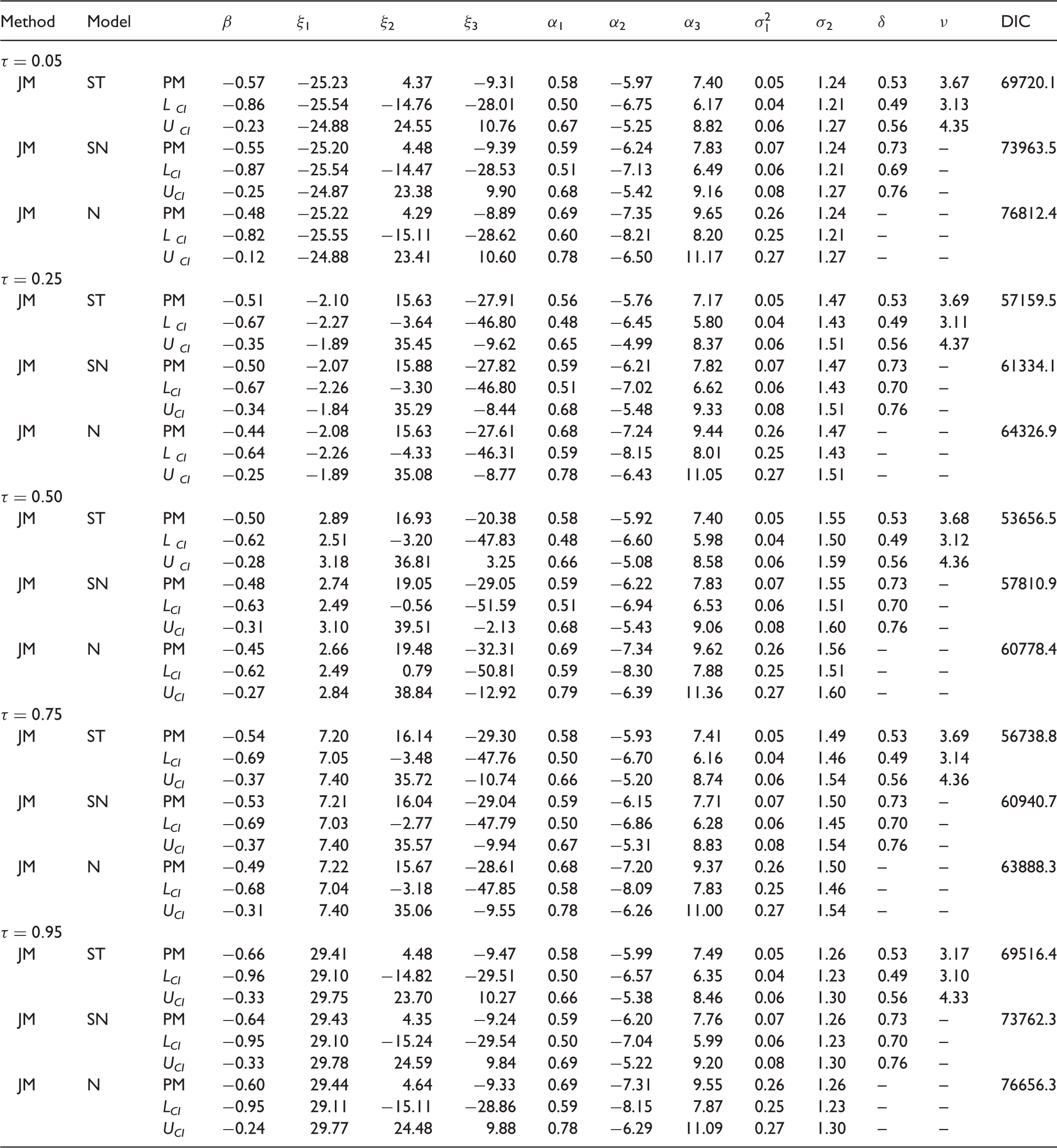
Bayesian joint modeling approach in conjunction with the QR-PLMJM at the five quantiles of

τ = 0.05, 0.25, 0.50, 0.75

and 0.95 was applied to fit the longitudinal viral load and CD4 data jointly. Table 1 presents the population posterior mean (PM), and the corresponding 95% credible interval (CI) for fixed-effects parameters based on the three proposed models (ST, SN and N). The following findings are obtained for the results of estimated parameters.

Table 1.

Summary of estimated posterior mean (PM) of population (fixed-effects) parameters, the corresponding lower limit (L_CI) and upper limit (U_CI) of 95% equal-tail credible interval (CI) as well as DIC values.

Method	Model		β	ξ ₁	ξ ₂	ξ ₃	α ₁	α ₂	α ₃	$σ_{1}^{2}$	σ ₂	δ	ν	DIC
$τ = 0.05$
JM	ST	PM	−0.57	−25.23	4.37	−9.31	0.58	−5.97	7.40	0.05	1.24	0.53	3.67	69720.1
		L _CI	−0.86	−25.54	−14.76	−28.01	0.50	−6.75	6.17	0.04	1.21	0.49	3.13
		U _CI	−0.23	−24.88	24.55	10.76	0.67	−5.25	8.82	0.06	1.27	0.56	4.35
JM	SN	PM	−0.55	−25.20	4.48	−9.39	0.59	−6.24	7.83	0.07	1.24	0.73	–	73963.5
		L_CI	−0.87	−25.54	−14.47	−28.53	0.51	−7.13	6.49	0.06	1.21	0.69	–
		U_CI	−0.25	−24.87	23.38	9.90	0.68	−5.42	9.16	0.08	1.27	0.76	–
JM	N	PM	−0.48	−25.22	4.29	−8.89	0.69	−7.35	9.65	0.26	1.24	–	–	76812.4
		L _CI	−0.82	−25.55	−15.11	−28.62	0.60	−8.21	8.20	0.25	1.21	–	–
		U _CI	−0.12	−24.88	23.41	10.60	0.78	−6.50	11.17	0.27	1.27	–	–
$τ = 0.25$
JM	ST	PM	−0.51	−2.10	15.63	−27.91	0.56	−5.76	7.17	0.05	1.47	0.53	3.69	57159.5
		L _CI	−0.67	−2.27	−3.64	−46.80	0.48	−6.45	5.80	0.04	1.43	0.49	3.11
		U _CI	−0.35	−1.89	35.45	−9.62	0.65	−4.99	8.37	0.06	1.51	0.56	4.37
JM	SN	PM	−0.50	−2.07	15.88	−27.82	0.59	−6.21	7.82	0.07	1.47	0.73	–	61334.1
		L_CI	−0.67	−2.26	−3.30	−46.80	0.51	−7.02	6.62	0.06	1.43	0.70	–
		U_CI	−0.34	−1.84	35.29	−8.44	0.68	−5.48	9.33	0.08	1.51	0.76	–
JM	N	PM	−0.44	−2.08	15.63	−27.61	0.68	−7.24	9.44	0.26	1.47	–	–	64326.9
		L _CI	−0.64	−2.26	−4.33	−46.31	0.59	−8.15	8.01	0.25	1.43	–	–
		U _CI	−0.25	−1.89	35.08	−8.77	0.78	−6.43	11.05	0.27	1.51	–	–
$τ = 0.50$
JM	ST	PM	−0.50	2.89	16.93	−20.38	0.58	−5.92	7.40	0.05	1.55	0.53	3.68	53656.5
		L _CI	−0.62	2.51	−3.20	−47.83	0.48	−6.60	5.98	0.04	1.50	0.49	3.12
		U _CI	−0.28	3.18	36.81	3.25	0.66	−5.08	8.58	0.06	1.59	0.56	4.36
JM	SN	PM	−0.48	2.74	19.05	−29.05	0.59	−6.22	7.83	0.07	1.55	0.73	–	57810.9
		L_CI	−0.63	2.49	−0.56	−51.59	0.51	−6.94	6.53	0.06	1.51	0.70	–
		U_CI	−0.31	3.10	39.51	−2.13	0.68	−5.43	9.06	0.08	1.60	0.76	–
JM	N	PM	−0.45	2.66	19.48	−32.31	0.69	−7.34	9.62	0.26	1.56	–	–	60778.4
		L_CI	−0.62	2.49	0.79	−50.81	0.59	−8.30	7.88	0.25	1.51	–	–
		U_CI	−0.27	2.84	38.84	−12.92	0.79	−6.39	11.36	0.27	1.60	–	–
$τ = 0.75$
JM	ST	PM	−0.54	7.20	16.14	−29.30	0.58	−5.93	7.41	0.05	1.49	0.53	3.69	56738.8
		L_CI	−0.69	7.05	−3.48	−47.76	0.50	−6.70	6.16	0.04	1.46	0.49	3.14
		U_CI	−0.37	7.40	35.72	−10.74	0.66	−5.20	8.74	0.06	1.54	0.56	4.36
JM	SN	PM	−0.53	7.21	16.04	−29.04	0.59	−6.15	7.71	0.07	1.50	0.73	–	60940.7
		L_CI	−0.69	7.03	−2.77	−47.79	0.50	−6.86	6.28	0.06	1.45	0.70	–
		U_CI	−0.37	7.40	35.57	−9.94	0.67	−5.31	8.83	0.08	1.54	0.76	–
JM	N	PM	−0.49	7.22	15.67	−28.61	0.68	−7.20	9.37	0.26	1.50	–	–	63888.3
		L_CI	−0.68	7.04	−3.18	−47.85	0.58	−8.09	7.83	0.25	1.46	–	–
		U_CI	−0.31	7.40	35.06	−9.55	0.78	−6.26	11.00	0.27	1.54	–	–
$τ = 0.95$
JM	ST	PM	−0.66	29.41	4.48	−9.47	0.58	−5.99	7.49	0.05	1.26	0.53	3.17	69516.4
		L_CI	−0.96	29.10	−14.82	−29.51	0.50	−6.57	6.35	0.04	1.23	0.49	3.10
		U_CI	−0.33	29.75	23.70	10.27	0.66	−5.38	8.46	0.06	1.30	0.56	4.33
JM	SN	PM	−0.64	29.43	4.35	−9.24	0.59	−6.20	7.76	0.07	1.26	0.73	–	73762.3
		L_CI	−0.95	29.10	−15.24	−29.54	0.50	−7.04	5.99	0.06	1.23	0.70	–
		U_CI	−0.33	29.78	24.59	9.84	0.69	−5.22	9.20	0.08	1.30	0.76	–
JM	N	PM	−0.60	29.44	4.64	−9.33	0.69	−7.31	9.55	0.26	1.26	–	–	76656.3
		L_CI	−0.95	29.11	−15.11	−28.86	0.59	−8.15	7.87	0.25	1.23	–	–
		U_CI	−0.24	29.77	24.48	9.88	0.78	−6.29	11.09	0.27	1.30	–	–

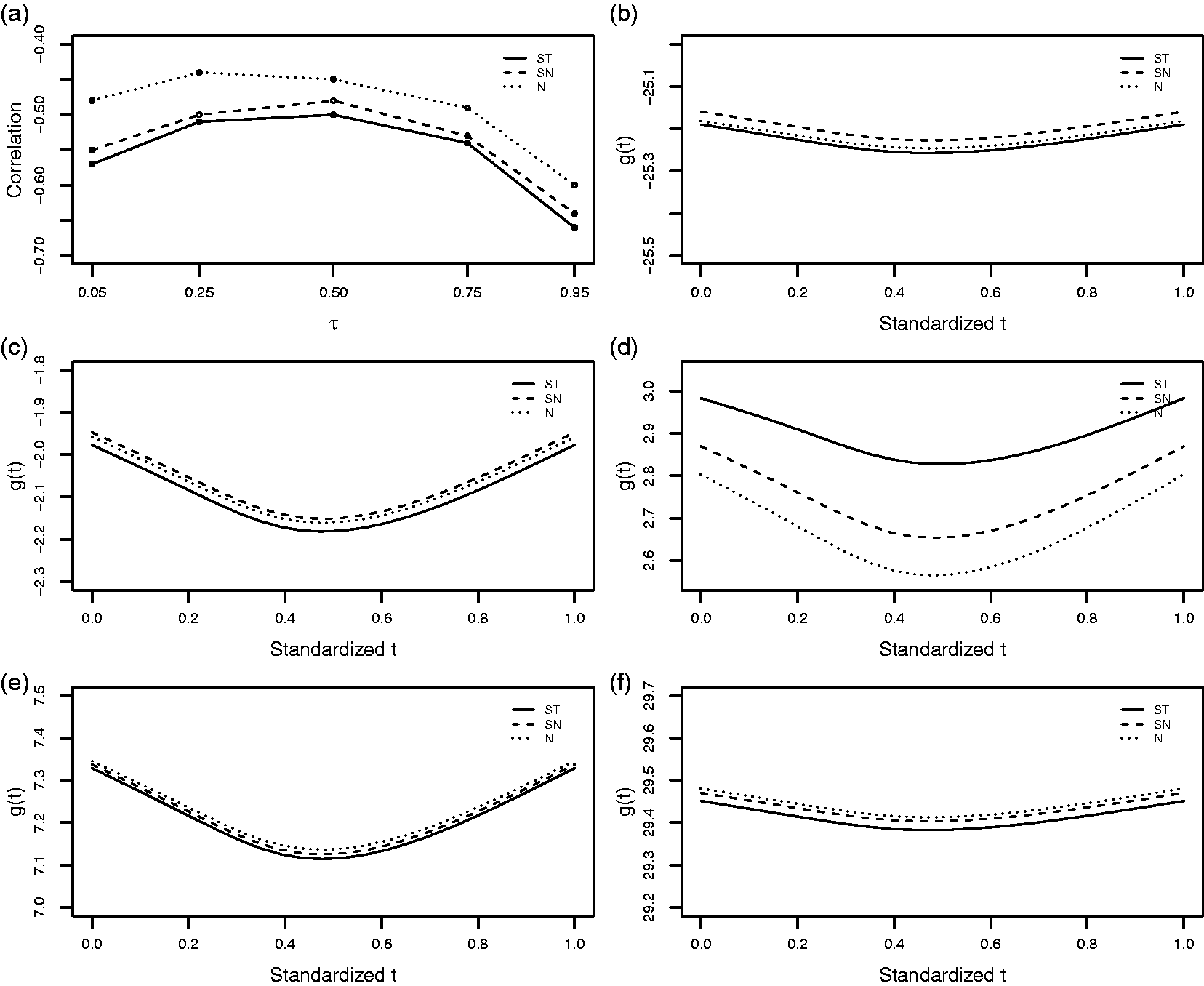
For all models ST, SN, and N with the five quantiles of $τ = 0.05, 0.25, 0.50, 0.75$ and 0.95 based on QR-PLMJM, first, it is interesting that the estimates of the key parameter β, that quantifies the effect of CD4 cell counts on viral load, are all significant but with different negative values. The results suggest a varying negative relationship between viral load and CD4 counts in the population level at different quantiles, while the estimated values of β reveal a “flat arch” shape (Figure 2(a)). Under the same models, the estimated value of β is the largest at median ( $τ = 0.50$ ), and decrease as quantile goes extremely (in both directions) with the smallest value at $τ = 0.95$ . Second, in comparison of Models ST, SN and N at the same quantile of τ, the values of estimated β at different quantiles in Model ST are smaller than their counterparts in Models SN and N, whereas those in Model N are the largest. This finding may indicate an underestimated negative CD4 effect by employing a joint model in which covariate model errors follow normal or SN distribution. Third, for the parameters in the nonparametric part of PLMM, as τ increases, the estimates of ξ₁ increase; from low quantiles to the median, the estimates of ξ₂ increase; reversely, from the median to high quantiles, the estimates of ξ₂ decrease. Fourth, from the population estimating nonparametric function g(t) at five different quantiles (Figure 2(b) to (f)), it is seen that, generally, g(t) decreases initially and then rebounds, but the decrease and rebound rates are smaller when $τ = 0.05$ and 0.95, compared to those at other quantiles. Though there are slight deviations among the estimated g(t) curves of different models, the estimates of parameters in the nonparametric part are comparable, except those at $τ = 0.50$ .

Figure 2.

(a) Strength of the correlation between viral load and CD4 counts under different scenarios; (b to f): The population estimating curves of g(t) based on the three models at five different quantiles, respectively.

In general, the estimated results for the parameters in the covariate model (2) at the five quantiles are comparable. The estimates of the linear coefficient α₂ are significantly negative, whereas the estimates of α₁ and α₃ are significantly positive. This finding suggests that there is a negative linear relationship between CD4 cell counts and measurement time. In comparison of Models ST, SN and N at the same quantile of τ, the estimated α₁ and α₃ in Model N are larger than their counterparts in Model ST and SN, while the estimated α₂ in Model N are smaller than their counterparts in Model ST and SN. However, the estimates of α₁ in Models ST and SN are comparable, and the estimated α₂ and α₃ vary slightly. Furthermore, it is noted that the estimated skewness parameter δ has a significantly positive value in Models SN and ST. This finding suggests that there is a significantly positive skewness on the CD4 data and confirms the fact that the distribution of the original CD4 data is right-skewed. Thus, incorporating a skewness parameter in the modeling of the CD4 covariate data is highly recommended. Interestingly, the estimated δ in Model ST is smaller than that in Model SN. It could be explained by adding one more parameter, degrees of freedom ν, in Model ST, which is significantly positive. Also, due to the consideration of skewness in both Models SN and ST, it is no surprising to see the great reduction for the estimates of scale parameter $σ_{1}^{2}$ .

To further select the best model that fits the data adequately, a Bayesian selection criterion, known as deviance information criterion (DIC),⁴⁸ is adopted. With caution here, DIC, which is not intended to identify the “correct” model, is only used to find the one fits the data best. In order to compare models under different settings, the DIC values obtained are also summarized in Table 1. It is seen that the DIC values in Model ST are smaller than their counterparts in Models SN and N at the same quantile of τ. Within any one of these three models, the DIC value is the smallest at the quantile of $τ = 0.50$ , whereas the DIC value is the largest at the quantile of $τ = 0.05$ . This may suggest that the smaller amount of information is available at more extreme quantiles (e.g. $τ = 0.05$ or $τ = 0.95$ ). Therefore, according to the DIC, the ST model-based median regression ( $τ = 0.50$ ) is the best fitting model, because of the smallest DIC (53656.5). In summary, our results suggest that it is important to assume an ST distribution for the covariate model in order to achieve more reliable results, particularly when the CD4 data exhibits non-normality.

For a specific application, we further report findings based on the best fitted model, Model ST in detail. First, the estimated coefficient of CD4 cell counts, β, varies from − 0.50 with 95%CI: (−0.62,−0.28) at $τ = 0.50$ to −0.66 with 95%CI: (−0.96, −0.33) at $τ = 0.95$ . It may be interpreted by the fact that, as CD4 cell counts increase one unit, the median of viral load ( ${log}_{10}$ transformed) will decrease by 0.5, but the 95th quantile will decrease by 0.66 at a given time, and both of these negative associations are statistically significant. This finding indicates that for the AIDS patients with high-level viral load, the effect of CD4 counts is stronger than other patients. In other words, the HIV treatment antiretroviral therapy (ART) may be more effective among severe AIDS patients. Additionally, the absolute value of the estimated β at $τ = 0.05$ is also relatively high $(β = - 0.57, 95 % CI : [- 0.86, - 0.23])$ , which could be partially explained by the fact that in the early stages of HIV, patients may be more sensitive to the drugs. Second, when $τ = 0.50$ , the estimated results indicate that the population CD4 trajectory may be approximated by the quadratic polynomial LME model: ${\hat{z}}^{*} (t) = 325.01 (0.58 - 5.92 t + 7.40 t^{2}) + 556.25$ , where ${\hat{z}}^{*} (t)$ is in the original CD4 scale. The population viral load process may be approximated by the PLMM: $\hat{V} (t) = - 0.50 {\hat{z}}^{*} (t) + 2.89 ψ_{0} (t) + 16.93 ψ_{1} (t) - 20.38 ψ_{2} (t)$ . Remind that this simple approximation considered here may provide a rough guidance and point to further research even though the true association described above may be complicated. The above findings may not be revealed from traditional mean regression models. An interesting note that we would make is that a quadratic relationship was found between estimated values of β and corresponding quantiles τ in this study, which can be mathematically expressed as $β = - 0.60 + 0.50 τ - 0.60 τ^{2}$ .

5 Simulation studies

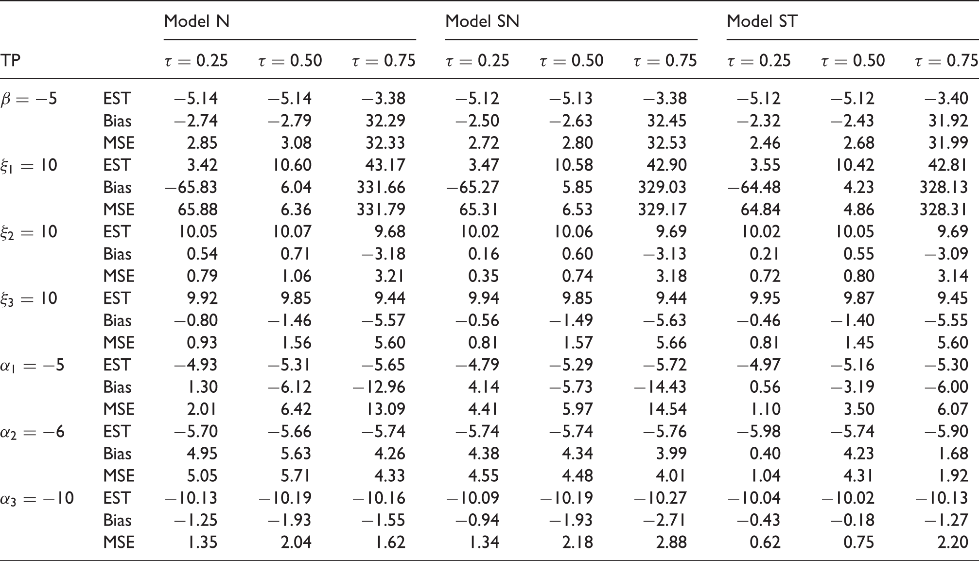
To evaluate the performance of our proposed QR-PLMJM and method, we conducted the following simulation studies. The design of the simulated data is similar to the real data used for the QR-PLMJM. Specifically, we adopted the sample size with n = 300, and assumed that each subject had 23 scheduled longitudinal measurements. The measurement time points generated in the simulation mimicked those in the real data analysis, and the true parameter values are selected as follows:

β = - 5, ξ_{3} = (ξ_{1}, ξ_{2}, ξ_{3})^{T} = (10, 10, 10)^{T}, α = (α_{1}, α_{2}, α_{3})^{T} = (- 5, - 6, - 10)^{T}

ϖ_{i} \sim N (0, diag (1, 1, 1, 1))

. The time-varying CD4 covariate z_ij is generated based on equation (2) with

(a_{i 1}, a_{i 2}, a_{i 3})^{T} \sim N (0, diag (1, 1, 1))

; we simulated the model errors e_ij and ε _ij from a

Γ (2, 1)

distribution, then subtracted by 2, which yields a skewed distribution with the mean 0 and variance 2. To simulate LOD data, we selected the 15% quantile of the longitudinal response as a cut-of threshold so that 15% of the data are below LOD. According to the settings described above, we generated 50 data sets due to intensive computation, and fitted the data by Models N, SN and ST at three different quantiles of

τ = 0.25, 0.50

and 0.75. Note that the prior distributions considered are all close to non-informative as they were treated in real data analysis. Therefore, we expect the results to be somewhat robust with respect to prior distributions. Table 2 summarizes the simulation results which include the true parameter (TP) values, percent bias (defined by

100 \times {bias}_{l} / | {TP}_{l} |

) and percent mean-square-error (MSE) (defined by

100 \times {\sqrt{MSE}}_{l} / | {TP}_{l} |

) of fixed-effects β,

ξ_{3}

, and

α

Table 2.

Summary of true parameter (TP) values, estimated parameters, Bias and MSE for Models N, SN and ST based on 100 simulated data sets under response model error with $Γ (2, 1)$ distribution and covariate model error with $Γ (2, 1)$ . EST is average of estimates, Bias and MSE are quantified by percent bias $= 100 \times {bias}_{l} / | {TP}_{l} |$ and percent $\sqrt{MSE} = 100 \times \sqrt{{MSE}_{l}} / | {TP}_{l} |$ , respectively.

		Model N			Model SN			Model ST
TP		$τ = 0.25$	$τ = 0.50$	$τ = 0.75$	$τ = 0.25$	$τ = 0.50$	$τ = 0.75$	$τ = 0.25$	$τ = 0.50$	$τ = 0.75$
$β = - 5$	EST	−5.14	−5.14	−3.38	−5.12	−5.13	−3.38	−5.12	−5.12	−3.40
	Bias	−2.74	−2.79	32.29	−2.50	−2.63	32.45	−2.32	−2.43	31.92
	MSE	2.85	3.08	32.33	2.72	2.80	32.53	2.46	2.68	31.99
$ξ_{1} = 10$	EST	3.42	10.60	43.17	3.47	10.58	42.90	3.55	10.42	42.81
	Bias	−65.83	6.04	331.66	−65.27	5.85	329.03	−64.48	4.23	328.13
	MSE	65.88	6.36	331.79	65.31	6.53	329.17	64.84	4.86	328.31
$ξ_{2} = 10$	EST	10.05	10.07	9.68	10.02	10.06	9.69	10.02	10.05	9.69
	Bias	0.54	0.71	−3.18	0.16	0.60	−3.13	0.21	0.55	−3.09
	MSE	0.79	1.06	3.21	0.35	0.74	3.18	0.72	0.80	3.14
$ξ_{3} = 10$	EST	9.92	9.85	9.44	9.94	9.85	9.44	9.95	9.87	9.45
	Bias	−0.80	−1.46	−5.57	−0.56	−1.49	−5.63	−0.46	−1.40	−5.55
	MSE	0.93	1.56	5.60	0.81	1.57	5.66	0.81	1.45	5.60
$α_{1} = - 5$	EST	−4.93	−5.31	−5.65	−4.79	−5.29	−5.72	−4.97	−5.16	−5.30
	Bias	1.30	−6.12	−12.96	4.14	−5.73	−14.43	0.56	−3.19	−6.00
	MSE	2.01	6.42	13.09	4.41	5.97	14.54	1.10	3.50	6.07
$α_{2} = - 6$	EST	−5.70	−5.66	−5.74	−5.74	−5.74	−5.76	−5.98	−5.74	−5.90
	Bias	4.95	5.63	4.26	4.38	4.34	3.99	0.40	4.23	1.68
	MSE	5.05	5.71	4.33	4.55	4.48	4.01	1.04	4.31	1.92
$α_{3} = - 10$	EST	−10.13	−10.19	−10.16	−10.09	−10.19	−10.27	−10.04	−10.02	−10.13
	Bias	−1.25	−1.93	−1.55	−0.94	−1.93	−2.71	−0.43	−0.18	−1.27
	MSE	1.35	2.04	1.62	1.34	2.18	2.88	0.62	0.75	2.20

For all scenarios considered in this simulation study, it is of interest to see that the estimated biases of parameter β in the parametric part of PLMM are negative when $τ = 0.25$ and 0.50, and positive when $τ = 0.75$ . The differences among the estimated β at different τ confirm that QR-based models can be used to detect the heterogeneous effects of covariate at different quantiles of the outcome. In the nonparametric part, the magnitude of ξ₁ increases as τ becomes larger. The big bias of this intercept parameter at $τ = 0.25$ and 0.75 is understandable in QR-based model, which is consistent with the results of real data analysis. Besides, the sign of the bias suggests that ξ₂ appears overestimated except when $τ = 0.75$ , and ξ₃ seems to be underestimated with the increasing bias as τ increases. Additionally, in comparison of Models ST, SN and N at the same quantile of τ, Model ST outperforms Models SN and N in terms of smaller bias and MSE, excluding ξ₂ at $τ = 0.25$ (in this scenario, Model SN seems to be the best). For parameters in covariate model, it can be observed that Model ST performs obviously better than Models N and SN because of the smaller bias and MSE. Specifically, the bias of $α$ ranges from −6.00% to 4.23% in Model ST, while bias ranges from −12.96% to 5.63% and from −14.43% to 4.38% in Models N and SN, respectively. In summary, the simulation study suggests that it is critical to account for skewness/heavy tails exhibited in the covariate by assuming an ST distribution.

6 Concluding discussion

To comprehensively study the complicated relationship between viral load and CD4 cell counts and the complex viral load trajectories at both population and individual levels, we presented a QR-PLMJM which is a special case of QR-based semiparametric models. We also considered some important data features which may affect the discovery of the longitudinal process, including CD4 covariate measurement errors, skewness, and viral load below LOD. A full Bayesian inference approach, which is powerful when the dimension of parameters in such complicated joint models is high, was adopted to get the point estimates and credible intervals for parameters of interest. To the best of our knowledge, this is the first time of jointly modelling QR-based PLMM, and covariate measurement error model, accounting for multiple longitudinal data features simultaneously. Although this study is motivated by MACS data, the novel models and method have broader applications and flexibility for practitioners to analyze complex longitudinal data under relevant specifications.

The proposed QR-PLMJM has many advantages compared to traditional mean-regression models, and pure parametric or nonparametric models. First, the parametric part of our QR-PLMJM detected the varying strength of CD4 effect on viral load at different quantiles, which gives researchers and physicians a full understanding of this significantly negative relationship. Specifically, the strongest negative effect was found at quantile $τ = 0.95$ , indicating that the effect of CD4 counts is more important among patients with higher viral load, which is consistent with biological mechanism. In other words, it may suggest that antiretroviral treatment (ART) is more effective for those patients with higher risk. Interestingly, the results also showed that the CD4 effect is relatively stronger at lower quantile $τ = 0.05$ . In this circumstance, the result suggests that, once the disease is discovered (when the viral load level of patients is low), the infected patients should be treated as soon as possible, because these patients may be more sensitive to the treatment in early stages of treatment. These findings may be undetectable via traditional mean-regression models. Second, the nonparametric part of the QR-PLMJM has the flexibility to model the viral dynamics by avoiding parametric misspecification, in order to monitor disease process accurately. More than that, it is pretty useful to observe the heterogeneous viral load trajectories at different quantiles. Compared to mean-regression models, it is more precise for physicians to evaluate treatment and make clinical decisions in accordance with the idea of “precision medicine”.

As one of the most important sources to clear out HIV virus, it is important to consider CD4 cell counts measurement error appropriately when it exhibits skewness and heavy tails. This study considered three models (Models N, SN and ST) with different scenarios, and found that Model ST is favorable in general to other two models. For the covariate model with ST distribution, the estimates of skewness parameter δ and the degrees of freedom ν are around 0.53 and 3.68, respectively, indicating positive skewness with heavy tail of the CD4 cell counts. Compared to Model SN, the magnitude of estimated δ is smaller in Model ST. This may be explained by the fact that the additional parameter ν for heaviness in the tails of ST distribution reduced the effect of skewness. The simulation studies also confirmed the results of real data analysis that Model ST gains more efficiency and accuracy in parameter estimation when covariate is in presence of skewness and heavy tails.

In Bayesian analysis, sensitivity analysis is important to check the changes of the posterior estimates when assuming different priors. Towards to the end, we performed sensitivity analysis by adopting a few sets of different values for the hyper-parameters in (8) and re-run the MCMC sampling procedure. The similar results give us confidence that the posterior estimates are robust to the hyper-parameter values. Moreover, the lower order polynomial model (2), that we applied to approximate the CD4 covariate process, is empirical and may not be true for the unknown CD4 path. Thus, the fitted CD4 counts based on this model are “regularized” CD4 counts instead of the “true” values. It provides a way to alleviate measurement errors in observed CD4 counts.

In summary, this study proposed a new flexible joint model, QR-PLMJM, with advances in HIV/AIDS dynamics to fully quantify complicated HIV disease mechanism. Although the proposed models are complex and applicable to a wider field in practice, our models have the potential to be further extended to more complicated models: (i) joint models considering the missing covariates by applying simple non-ignorable model for missing mechanism^24,25; (ii) joint models for longitudinal-survival data.^25,35,39 These interesting problems are beyond the focus of this article, but are warranted in future research.

Footnotes

Acknowledgement

The authors gratefully acknowledge the Editor and two anonymous referees for their insightful comments and constructive suggestions that led to a marked improvement of the article.

Declaration of conflicting interests

The author(s) declared no potential conflicts of interest with respect to the research, authorship, and/or publication of this article.

Funding

The author(s) disclosed receipt of the following financial support for the research, authorship, and/or publication of this article: Y. Huang was partially supported by University South Florida Proposal Enhancement grant (18326).

Appendix 1. Multivariate skew distributions and asymmetric Laplace distribution

Appendix 2. R and WinBUGS program codes for Model ST

Appendix 3. Plots of convergence diagnostics for Model ST with τ = 0 . 5 quantile

References

. A joint model for nonlinear mixed-effects models with censoring and covariates measured with error, with application to aids studies. J Am Stat Assoc 2002; 97: 955–964.

Liu

. Simultaneous inference for semiparametric nonlinear mixed-effects models with covariate measurement errors and missing responses. Biometrics 2007; 63: 342–350.

Liu

. Joint inference on HIV viral dynamics and immune suppression in presence of measurement errors. Biometrics 2010; 66: 327–335.

Huang

Dagne

. A Bayesian approach to joint mixed-effects models with a skew-normal distribution and measurement errors in covariates. Biometrics 2011; 67: 260–269.

Liu

. Simultaneous inference and bias analysis for longitudinal data with covariate measurement error and missing responses. Biometrics 2011; 67: 67–75.

Kaslow

Ostrow

Detels

et al.

The Multicenter AIDS Cohort Study: rationale, organization, and selected characteristics of the participants. American Journal of Epidemiology 1987; 126: 310–318.

Koenker

Bassett

Jr . Regression quantiles. Econometrica: J Economet Soc 1978; 46: 33–50.

Davino

Furno

Vistocco

. Quantile regression: theory and applications, Chichester, United Kingdom: John Wiley & Sons, 2013.

Buchinsky

. Changes in the us wage structure 1963–1987: application of quantile regression. Econometrica: J Economet Soc 1994; 62: 405–458.

10.

Cade

Noon

. A gentle introduction to quantile regression for ecologists. Front Ecol Environ 2003; 1: 412–420.

11.

Haque

Nehrir

Mandal

. A hybrid intelligent model for deterministic and quantile regression approach for probabilistic wind power forecasting. IEEE Transact Power Syst 2014; 29: 1663–1672.

12.

Lipsitz

Fitzmaurice

Molenberghs

et al.

Quantile regression methods for longitudinal data with drop-outs: Application to CD4 cell counts of patients infected with the human immunodeficiency virus. J Royal Stat Soc: Ser C (Appl Stat) 1997; 46: 463–476.

13.

Fung

. Median regression for longitudinal data. Stat Med 2003; 22: 3655–3669.

14.

Koenker

. Quantile regression for longitudinal data. J Multivariate Anal 2004; 91: 74–89.

15.

Wang

Fygenson

. Inference for censored quantile regression models in longitudinal studies. Ann Stat 2009; 37: 756–781.

16.

Farcomeni

. Quantile regression for longitudinal data based on latent Markov subject-specific parameters. Stat Comput 2012; 22: 141–152.

17.

Geraci

Bottai

. Quantile regression for longitudinal data using the asymmetric Laplace distribution. Biostat 2007; 8: 140–154.

18.

Liu

Bottai

. Mixed-effects models for conditional quantiles with longitudinal data. Int J Biostat 2009; 5: Article 28–28.

19.

Farcomeni

Viviani

. Longitudinal quantile regression in the presence of informative dropout through longitudinal-survival joint modeling. Stat Med 2015; 34: 1199–1213.

20.

Yuan

Yin

. Bayesian quantile regression for longitudinal studies with nonignorable missing data. Biometrics 2010; 66: 105–114.

21.

Luo

Lian

Tian

. Bayesian quantile regression for longitudinal data models. J Stat Comput Simul 2012; 82: 1635–1649.

22.

Kim

Yang

. Semiparametric approach to a random effects quantile regression model. J Am Stat Assoc 2012; 106: 1405–1417.

23.

Tian

. Bayesian joint quantile regression for mixed effects models with censoring and errors in covariates. Computat Stat 2015; 31: 1031–1057.

24.

Huang

. Quantile regression-based Bayesian semiparametric mixed-effects models for longitudinal data with non-normal, missing and mismeasured covariate. J Stat Comput Simul 2016; 86: 1183–1202.

25.

Huang

Chen

. Bayesian quantile regression-based nonlinear mixed-effects joint models for time-to-event and longitudinal data with multiple features. Stat Med 2016; 35: 5666–5685.

26.

Liang

Zeger

. Longitudinal data analysis using generalized linear models. Biometrika 1986; 73: 13–22.

27.

Diggle

. Analysis of longitudinal data, Oxford, United Kingdom: Oxford University Press, 2002.

28.

Härdle

Liang

. Partially linear models. In: Statistical methods for biostatistics and related fields, Heidelberg, Germany: Springer, 2007, pp. 87–103.

29.

Liang

Ren

. Generalized partially linear measurement error models. J Computat Graph Stat 2005; 14: 237–250.

30.

Liang

. Generalized partially linear mixed-effects models incorporating mismeasured covariates. Ann Inst Stat Math 2009; 61: 27–46.

31.

Huang

. Bayesian inference on partially linear mixed-effects joint models for longitudinal data with multiple features. Computat Stat 2017; 32: 179–196.

32.

Dagne

Huang

. Mixed-effects Tobit joint models for longitudinal data with skewness, detection limits, and measurement errors. J Probabil Stat 2011; 2012: 1–19.

33.

Dagne

Huang

. Bayesian inference for a nonlinear mixed-effects Tobit model with multivariate skew-t distributions: application to AIDS studies. Int J Biostat 2012; 8: Article 27–27.

34.

Demirtas

Freels

Yucel

. Plausibility of multivariate normality assumption when multiply imputing non-Gaussian continuous outcomes: a simulation assessment. J Stat Comput Simul 2008; 78: 69–84.

35.

Huang

Dagne

. Bayesian inference on joint models of HIV dynamics for time-to-event and longitudinal data with skewness and covariate measurement errors. Stat Med 2011; 30: 2930–2946.

36.

Oberg

Davidian

. Estimating data transformations in nonlinear mixed effects models. Biometrics 2000; 56: 65–72.

37.

Sahu

Dey

Branco

. A new class of multivariate skew distributions with applications to Bayesian regression models. Can J Stat 2003; 31: 129–150.

38.

Zhang

. A three-parameter asymmetric Laplace distribution and its extension. Commun Stat Theory Meth 2005; 34: 1867–1879.

39.

Chen

May

Ibrahim

et al.

Joint modeling of longitudinal and survival data with missing and left-censored time-varying covariates. Stat Med 2014; 33: 4560–4576.

40.

Carroll

Ruppert

Stefanski

et al.

Measurement error in nonlinear models: a modern perspective, Boca Raton, FL: CRC Press, 2006.

41.

Ding

. Population HIV-1 dynamics in vivo: applicable models and inferential tools for virological data from AIDS clinical trials. Biometrics 1999; 55: 410–418.

42.

Huang

Liu

. Hierarchical Bayesian methods for estimation of parameters in a longitudinal HIV dynamic system. Biometrics 2006; 62: 413–423.

43.

Davidian

Giltinan

. Nonlinear models for repeated measurement data 1995; Vol. 62, Boca Raton, FL: CRC Press.

44.

Zhang

. Nonparametric regression methods for longitudinal data analysis: mixed-effects modeling approaches 2006; Vol. 515, Hoboken, NJ: John Wiley & Sons.

45.

Brown

Ibrahim

. A Bayesian semiparametric joint hierarchical model for longitudinal and survival data. Biometrics 2003; 59: 221–228.

46.

Lunn

Thomas

Best

et al.

WinBUGS-a Bayesian modelling framework: concepts, structure, and extensibility. Stat Comput 2000; 10: 325–337.

47.

Gelman

Rubin

. Inference from iterative simulation using multiple sequences. Stat Sci 1992; 7: 457–472.

48.

Spiegelhalter

Best

Carlin

et al.

Bayesian measures of model complexity and fit. J Royal Stat Soc: Ser B (Stat Methodol) 2002; 64: 583–639.

49.

Arellano-Valle

Genton

. On fundamental skew distributions. J Multivariate Anal 2005; 96: 93–116.

50.

Arellano-Valle

Bolfarine

Lachos

. Bayesian inference for skew-normal linear mixed models. J Appl Stat 2007; 34: 663–682.

51.

Azzalini

Capitanio

. Statistical applications of the multivariate skew normal distribution. J Royal Stat Soc: Ser B (Stat Methodol) 1999; 61: 579–602.

52.

Azzalini

Capitanio

. Distributions generated by perturbation of symmetry with emphasis on a multivariate skew t-distribution. J Royal Stat Soc: Ser B (Stat Methodol) 2003; 65: 367–389.

53.

Jara

Quintana

San Martín

. Linear mixed models with skew-elliptical distributions: A Bayesian approach. Comput Stat Data Anal 2008; 52: 5033–5045.

54.

Lachos

Ghosh

Arellano-Valle

. Likelihood based inference for skew-normal independent linear mixed models. Stat Sinica 2010; 20: 303–322.

55.

Koenker

Machado

. Goodness of fit and related inference processes for quantile regression. J Am Stat Assoc 1999; 94: 1296–1310.

56.

Moyeed

. Bayesian quantile regression. Stat Prob Lett 2001; 54: 437–447.

57.

Stander

. Quantile regression: applications and current research areas. Journal of the Royal Stat Soc: Ser D (The Statistician) 2003; 52: 331–350.

58.

Johnson

Kotz

Balakrishnan

. Continuous univariate distributions 1995; Vol. 2, 2nd ed. New York, NY: Wiley.

59.

Kotz

Kozubowski

Podgórski

. Maximum likelihood estimation of asymmetric Laplace parameters. Ann Inst Stat Math 2002; 54: 816–826.

60.

Kotz

Kozubowski

Podgórski

. Asymmetric multivariate Laplace distribution. In: The Laplace distribution and generalizations, New York, NY: Springer, 2001, pp. 239–272.

61.

Kozumi

Kobayashi

. Gibbs sampling methods for Bayesian quantile regression. J Stat Comput Simul 2011; 81: 1565–1578.

62.

Kobayashi

Kozumi

. Bayesian analysis of quantile regression for censored dynamic panel data. Comput Stat 2012; 27: 359–380.

63.

Reich

Fuentes

Dunson

. Bayesian spatial quantile regression. J Am Stat Assoc 2012; 106: 6–22.

64.

Stander

. Bayesian analysis of a Tobit quantile regression model. J Economet 2007; 137: 260–276.