Shared parameter models for joint analysis of longitudinal and survival data with left truncation due to delayed entry

Abstract

Many longitudinal studies observe time to occurrence of a clinical event such as death, while also collecting serial measurements of one or more biomarkers that are predictive of the event, or are surrogate outcomes of interest. Joint modeling can be used to examine the relationship between the biomarker and the event, and also as a way of adjusting analyses of the biomarker for non-ignorable dropout. In settings such as registry studies, an additional complexity is caused when follow-up of subjects is delayed, referred to as left-truncation of follow-up in the survival analysis setting. If not adjusted for, this can cause bias in estimation of parameters of the survival distribution for the clinical event and in parameters of the longitudinal outcome such as the profile or rate of change over time because subjects may die or have the clinical event before follow-up starts. This paper illustrates how a broad class of shared parameter models can be used to jointly model a time to event outcome along with a longitudinal marker using available nonlinear mixed modeling software, when follow-up times are left truncated. Methods are applied to jointly model survival and decline in lung function in cystic fibrosis patients.

Keywords

Joint modeling non-ignorable dropout longitudinal studies cystic fibrosis nonlinear mixed models accelerated failure time models proportional hazards models piecewise exponential

1 Introduction

In many longitudinal studies, patients are followed to observe the time to occurrence of a clinical event of interest such as death, wherein addition serial measurements are made on a biomarker or surrogate outcome that is predictive of the event of interest. Joint modeling of time-to-event and longitudinal data has received considerable attention in the statistical literature as a means to: a) remove or reduce bias in estimating trends in the longitudinal biomarker caused by censoring of follow-up due to occurrence of the event (sometimes referred to as non-ignorable dropout or informative censoring), b) examine the relationship between the biomarker and the risk of occurrence of the clinical outcome, or c) improve estimation in either or both outcomes as compared to separate analyses of the two outcomes. Overviews of methodology and uses of joint modeling can be found in review articles,^1,2 a text by Rizopoulos,³ and a meta analysis of articles on joint modeling by Sudell et al.⁴

In some situations, not all patients are followed from time zero, which can occur for example in disease registries where follow-up does not begin on some patients until sometime after the time of diagnosis. When analyzing time-to-event data, methods for handling left truncated survival data in the parametric and semi- or nonparametric setting are well developed.^5–7 Although methods for analysis of longitudinal data of a serial biomarker when follow-up is left truncated has received less attention, recent papers have shown how it can be facilitated using joint modeling techniques.^8–12 Proust-Lima et al.¹¹ and Dantan et al.⁹ developed joint modeling approaches incorporating left truncation in the framework of latent class models and mulitistate models, respectively, and applied them to studies of cognitive decline in the elderly. van den Hout and Muniz-Terrera¹² developed a shared parameter model for a survival and a discrete ordinal longitudinal outcome and also applied the methods to studies of cognitive decline in a longitudinal study of ageing. Crowther et al.⁸ formulated a joint model combining a longitudinal mixed model for the longitudinal outcome with a proportional hazards survival model, allowing for left truncation or delayed entry. They proposed using flexible modeling techniques including use of polynomials or splines to model the longitudinal marker as well as the baseline hazard function, and made available Stata code.¹³ Piccorelli and Schluchter¹⁰ jointly modeled lung function measurements in the form of forced expiratory volume in one second as percent of predicted normal (%FEV₁) and survival in subjects with cystic fibrosis (CF). They developed a model that assumed lognormal survival times were correlated with the %FEV₁ longitudinal trajectory through shared subject-specific random intercept and slope random effects, and a corresponding EM algorithm that included a correction for left truncation due to late entry. They demonstrated that not adjusting for the left truncation resulted in biased estimation of intercepts and slopes of %FEV₁ as well as in estimated survival. In this paper, we extend this work, showing how the lognormal model previously examined, as well as a broader class of shared parameter joint models that includes both accelerated failure time and proportional hazards survival models can be fit using non-linear mixed model software. Our approach extends previous papers illustrating the fitting of shared parameter models using the NLMIXED procedure in SAS,^14–16 where we show how left truncation in the data can be accommodated using user-supplied code to calculate an additional term needed in the likelihood function, using Gaussian quadrature.

In the next section, we introduce notation and describe the basic model. Section 3 describes how maximum likelihood estimates of model parameters are obtained using nonlinear mixed modeling software. In Section 4, the approach is applied to analyze data consisting of longitudinal measurements of lung function and survival of subjects with cystic fibrosis. Section 5 deals with assessing model fit and validity of model assumptions. We provide some final comments in Section 6.

2 Model and notation

For subject i, i = 1,…,n, we observe $T_{i} = min (T_{i}^{0}, C_{i})$ where $T_{i}^{0}$ is the time to occurrence of the clinical event of interest and $C_{i}$ is a right censoring time, assumed independent of $T_{i}^{0}$ . Corresponding to T_i, we also observe the indicator variable $δ_{i} = I (T_{i} = T_{i}^{0})$ . We also let L_i denote the left truncation time or “time of entry” (time when follow-up began) for subject i, along with the indicator variable $I_{i}^{tr} = I (L_{i} > 0)$ , where L_i and $I_{i}^{tr}$ are assumed to be independent of $T_{i}^{0}$ . If no left truncation occurred for subject i, then $(L_{i}, I_{i}^{tr}) = (0, 0)$ ; otherwise $L_{i} > 0$ and $I_{i}^{tr} = 1$ . In addition we observe n_i measurements of a longitudinal biomarker y for subject i where $y_{it}$ is the measurement made at the tth time point, t = 1,…, n_i and $y_{i} = (y_{i 1}, y_{i 2}, \dots,, y_{{in}_{i}})$ is the $n_{i} x 1$ vector of responses for subject i. Note that subjects can differ with respect to the number of measurements taken as well as the actual times when measurements were taken.

We assume a shared parameter model for $T_{i}^{0}$ and $y_{i}$ , which combines a linear mixed model or generalized linear mixed model for the longitudinal outcome y with a parametric survival model for $T_{i}^{0}$ , where the models for $T_{i}^{0}$ and $y_{i}$ are linked by sharing a common set of random effects, denoted as $b_{i}$ = $(b_{1 i}, \dots,, b_{qi})'$ . This paper focuses on the case where the $y_{it}$ are continuous and normally distributed. The random effects in $b_{i}$ are assumed to have a multivariate normal distribution with mean vector 0 and covariance matrix $Σ$ . Conditional on $b_{i}$ , $T_{i}^{0}$ and $y_{i}$ are assumed to be independent, where their joint dependence on $b_{i}$ causes them to be correlated unconditionally.

The conditional distribution of $y_{i}$ given $b_{i}$ , denoted as $π_{y | b} (y_{i} | b_{i}; α, σ_{e}^{2})$ is described using a standard linear mixed model, expressed as

y_{i} = X_{i} α + Z_{i} b_{i} + e_{i}

(1)

where

X_{i}

and

Z_{i}

are known design matrices of dimension n_i × p and n_i × q, respectively,

α

is a p × 1 fixed effects parameter vector, and it is assumed

b_{i}

∼

N (0, Σ)

and

e_{i}

∼

N (0, σ_{e}^{2} I_{n_{i}})

where

b_{i}

and

e_{i}

are independent.

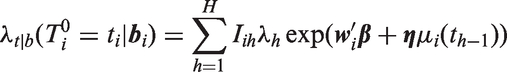
The conditional distribution of $T_{i}^{0}$ given $b_{i}$ is denoted $π_{t | b} (T_{i}^{0} | b_{i}; θ)$ , where $θ$ denotes a vector of unknown parameters of this distribution. Let $w_{i}$ denote an r × 1 vector of known covariates to be potentially included in the model as predictors of $T_{i}^{0}$ . Depending on the assumed underlying distribution for $T_{i}^{0}$ , either proportional hazards (PH) models or accelerated failure time (AFT) models can be fit, where effects of covariates in $w_{i}$ and the random effects in $b_{i}$ on survival are modeled through the linear predictor: $w'_{i} β + η' b_{i}$ . In the accelerated failure time (AFT) model, which includes cases where $T_{i}^{0}$ has a lognormal, gamma or Weibull distribution, the model can be expressed as

log (T_{i}^{0}) = w'_{i} β + η' b_{i} + ɛ_{i}

(2)

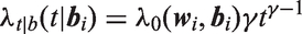
where the errors

ɛ_{i}

, i = 1,…,n are iid, with a distribution depending on an additional scale parameter. In the AFT model, a one unit increase in covariate

w_{s} \in w

with corresponding regression coefficient

β_{s} \in β

changes the survival time multiplicatively by the factor

e^{β_{s}}

, s = 1,…r. Similarly a one-unit increase in random effect

b_{ji} \in b_{i}

with coefficient

η_{j} \in η

changes survival by the factor

e^{η_{j}}

, j = 1,…,q. In the proportional hazards class, which includes the Weibull and piecewise exponential models, the distribution of

T_{i}^{0}

given

b_{i}

can be written in terms of the conditional hazard function

λ_{t | b} (t | b_{i}) = λ_{0} (t) exp (w'_{i} β + η' b_{i})

(3)

where

λ_{0} (t)

is a baseline hazard function. In the PH model, the factors

e^{β_{s}}

and

e^{η_{j}}

, respectively, are hazard ratios indicating the multiplicative change in the hazard function corresponding to a one-unit increase in the corresponding covariate

w_{s} \in w

or random effect

b_{ji} \in b_{i}

3 Maximum likelihood estimation of parameters

The observed data for the ith subject consist of ${y_{i}, T_{i}, δ_{i}, I_{i}^{tr}, L_{i}}$ , along with covariates and design variables in $X_{i}, Z_{i}$ and $w_{i}$ for i = 1,…,n. The contribution to the likelihood for subject i is

\begin{matrix} l_{i} (α, σ_{e}^{2}, Σ, θ; y_{i}, T_{i}, δ_{i}, L_{i}, I_{i}^{tr}) = S_{t} (L_{i})^{- I_{i}^{tr}} \int_{b_{i}} π_{y | b} (y_{i} | b_{i}; α, Σ, σ_{e}^{2}) π_{t | b} (T_{i} | b_{i}; θ)^{δ_{i}} S_{t | b} (T_{i} | b_{i}; θ)^{1 - δ_{i}} π (b_{i}; Σ) \partial b_{i} \end{matrix}

(4)

where

S_{t | b} (T_{i} | b_{i}; θ) = P (T_{i}^{0} > T_{i} | b_{i}) = \int_{T_{i}}^{\infty} π_{t | b} (t | b_{i}; θ) \partial t

(5)

\begin{matrix} S_{t} (L_{i}) = P (T_{i}^{0} > L_{i}) = \int_{b_{i}} \int_{L_{i}}^{\infty} π_{t | b} (t | b_{i}; θ) π (b_{i}; Σ) \partial t \partial b_{i} = \int_{b_{i}} S_{t | b} (L_{i} | b_{i}) π (b_{i}; Σ) \partial b_{i} \end{matrix}

(6)

π (b_{i}; Σ)

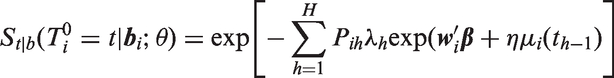
is the q-variate normal

N (0, Σ)

density, θ is a vector of parameters of the distribution of

T_{i}^{0} | b_{i}

including

β

and

η

, and

\int_{b_{i}}

denotes multiple integration over

b_{i 1}, \dots,, b_{iq} .

The only difference in the likelihood contribution for a subject whose survival time is left truncated (

L_{i}

> 0,

I_{i}^{tr} =

1), compared to a subject with no left truncation (

L_{i}

= 0,

I_{i}^{tr} =

0), is that the likelihood for the subject with truncated survival is divided by the term

S_{t} (L_{i})

which is the unconditional probability that

T_{i}^{0}

exceeds the truncation time

L_{i}

. Note that

S_{t} (L_{i})

and

S_{t} (L_{j})

may differ for two subjects i and j who have the same left truncation times, i.e.

L_{i} = L_{j}

, if their covariate vectors

w_{i}

and

w_{j}

or design matrices X _i and X _j differ. Because it is not conditional on

b_{i}

S_{t} (L_{i})

does not appear inside the integral in the likelihood in equation (4).

When using SAS PROC NLMIXED, the user provides code to calculate the terms $π_{y | b} (y_{i} | b_{i}; α, σ_{e}^{2}), π_{t | b} (T_{i} | b_{i}; θ), and S_{t | b} (T_{i} | b_{i}; θ)$ that appear inside the integral of the likelihood (4), while utilizing the built-in feature of the program specifying $b_{i}$ to have a multivariate normal distribution, where the program computes the integral over $b_{i}$ numerically using Gaussian quadrature. When standard survival distributions are specified for the conditional density $π_{t | b} (.),$ the hazard function and/or survival function of $T_{i}^{0}$ given $b_{i}$ are easily programmable using closed-form expressions and available functions in SAS. An additional required step when there is left truncation at time $L_{i}$ is to calculate $S_{t} (L_{i})$ , the marginal survival function of $T_{i}^{0}$ after integrating over $b_{i}$ . Except for special cases such as the lognormal AFT model described in the next section, closed-form expressions for $S_{t} (L_{i})$ do not exist. However, in a number of models such as the Weibull and Gamma models, $S_{t | b} (L_{i} | b_{i})$ depends on $b_{i}$ through a scalar linear function of the random effects $x_{i} = {l' b}_{i}$ , which itself has a normal distribution. $S_{t} (L_{i})$ can be then written as the expected value of a function of x_i, which can be approximated in the program using one-dimensional numerical integration. In other models such as the piecewise exponential model where $S_{t | b} (L_{i} | b_{i})$ does not depend on $b_{i}$ through a linear function, $S_{t} (L_{i})$ can be calculated using q-dimensional numerical integration. With the CF data we found empirically that 12-point Gaussian quadrature provided sufficient precision (see Appendix 1). Note that this number of quadrature points is not the same as the QPOINTS option in the PROC NLMIXED statement, discussed in the next paragraph.

Using default options, NLMIXED proceeds iteratively to find maximum likelihood estimates (MLEs) by using Gauss–Hermite quadrature to approximate the integrated likelihood (4), with use of a quasi-Newton algorithm to obtain updated parameter estimates. Initial estimates of parameters other than $η$ used in the estimation may be obtained by separately fitting the linear mixed model and parametric survival models. Initial values of $η$ can be zero, or can be chosen based on prior beliefs about the strength of association between $b_{i}$ and $T_{i}^{0}$ . The number of quadrature points (QPOINTS) is determined adaptively (the default) or can be specified by the user. For analyses presented here, we allowed the number of quadrature points to be determined adaptively by the program, and verified results in some cases by increasing QPOINTS as a sensitivity check.

4 Application to analysis of cystic fibrosis data

To illustrate the methods, we apply this modeling approach to data on longitudinal measurements of %FEV₁ and survival for patients included in a registry of patients with cystic fibrosis at Case Western Reserve University and Rainbow Babies and Children’s Hospital. These data have been previously described.¹⁰

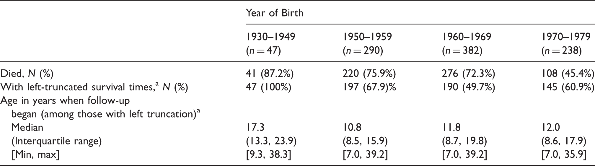
Because entry in the registry began when the subject first had pulmonary function measured, and pulmonary function tests (PFT’s) were not done in children younger than 6 years of age, we take time zero as age six, and define

T_{i}^{0}

to be survival time in years since the age of 6. If the age when a subject’s first PFT was measured was less than seven years, the subject was assumed to have been followed from time zero (age six) with no delayed entry (

L_{i}

= 0 and

I_{i}^{tr} = 0) .

Otherwise if the first PFT was at an age ≥ 7.0 the left truncation time was set to

L_{i}

= age at first PFT minus six. For this paper we restrict analysis to those subjects born between 1930 and 1979, and examine four birth cohorts: 1930–1949, 1950–1959, 1960–1969, and 1970–1979. Since the dataset was created in 2009, this ensured that all subjects in all cohorts potentially had at least 30 years of follow-up. The longitudinal outcome y is %FEV₁. If a subject had more than one pulmonary function test in a calendar year, we used the single PFT with the highest %FEV₁ per year.^10,17,18 The final dataset for this analysis consisted of 957 subjects (Table 1). This study and the ongoing parent cystic fibrosis registry, including procedures for obtaining informed consent, were approved by the University Hospitals Case Medical Center Institutional Review Board.

Table 1.

Description of the cystic fibrosis data.

	Year of Birth
	1930–1949 (n = 47)	1950–1959 (n = 290)	1960–1969 (n = 382)	1970–1979 (n = 238)
Died, N (%)	41 (87.2%)	220 (75.9%)	276 (72.3%)	108 (45.4%)
With left-truncated survival times,^a N (%)	47 (100%)	197 (67.9)%	190 (49.7%)	145 (60.9%)
Age in years when follow-up
began (among those with left truncation)^a
Median	17.3	10.8	11.8	12.0
(Interquartile range)	(13.3, 23.9)	(8.5, 15.9)	(8.7, 19.8)	(8.6, 17.9)
[Min, max]	[9.3, 38.3]	[7.0, 39.2]	[7.0, 39.2]	[7.0, 35.9]

Left truncation (delayed entry) was operationally defined as the subject having their first pulmonary function test at age ≥7 years.

As was done in previous analyses of these data,¹⁰ we focus on modeling a linear relationship between %FEV₁ and Age, allowing the intercepts and slopes of the line to differ among the four birth cohorts. The linear mixed model for y is written as

\begin{matrix} y_{it} | b_{i} = (α_{11} G_{1 i} + \dots + α_{14} G_{4 i} + b_{1 i}) + (α_{21} G_{1 i} + \dots + α_{24} G_{4 i} + b_{2 i}) ({Age}_{it} - 6) + e_{it} \end{matrix}

(7)

where

y_{it}

is the ith subject’s measurement of %FEV₁, measured at age Age_it,

G_{1 i}, \dots G_{4 i}

are 0/1 indicator variables defining which of the four birth cohorts subject i belongs to, where

α_{1 g}

and

α_{2 g}

, respectively, are the mean population intercept at age 6 and slope (in percentage predicted per year) of %FEV₁ for the gth birth cohort, g = 1,…,4 and

b_{i} = (b_{1 i}, b_{2 i})'

and

e_{i} = (e_{i 1}, e_{i 2}, \dots, e_{{in}_{i}})'

are as defined previously, i = 1,…n, t = 1,…,n_i. In this model, we center age at 6 years to improve computational efficiency, and because intercepts at age 6 (approximately the earliest age when spirometry can be performed in children) are meaningful, whereas intercepts at age 0 are not. Age could be centered at a value other than 6 years in the model for

y_{it} | b_{i}

in equation (7), noting that changing the centering value changes the interpretation and values of the parameters

σ_{11} = var (b_{1 i}), σ_{12} = cov (b_{1 i}, b_{2 i})

, and

η_{1}

and

η_{2}

. The distribution of time in years from age 6 to death conditional on the random effects b_i is modeled using several parametric models, as illustrated below. Code for fitting these models in PROC NLMIXED is included and explained in the Supplemental Materials.

4.1 Lognormal model

The lognormal AFT model assumes that, conditional on $b_{i}$ , $log (T_{i}^{0})$ has a normal distribution

log (T_{i}^{0}) \sim N (w'_{i} β + η' b_{i}, σ_{t | b}^{2})

(8)

In models fit to the CF data, $w'_{i} β = \sum_{g} G_{gi} β_{g},$ which equals $β_{g}$ (the mean of $log (T_{i}^{0})$ for birth cohort g) when subject i belongs to cohort g, g = 1,…,4. Parameters of the distribution of $T_{i}^{0} | b_{i}$ are $θ' = (β^{'}, η', σ_{t | b}^{2})$ . The shared parameter model defined by equations (7) and (8) is equivalent to a lognormal model fit to cystic fibrosis data using an EM algorithm developed to accommodate left-truncated data¹⁰ and previously used in other studies of cystic fibrosis and renal disease.^17,19,20 If $b_{i}^{true} = (b_{1 i}^{true}, b_{2 i}^{true})'$ denotes the true intercept and slope of the regression of y vs. time for the ith subject, i.e.

b_{i}^{true} = (\begin{matrix} b_{1 i}^{true} \\ b_{2 i}^{true} \end{matrix}) = (\begin{matrix} α_{11} G_{1 i} + \dots + α_{14} G_{4 i} + b_{i 1} \\ α_{21} G_{1 i} + \dots + α_{24} G_{4 i} + b_{i 2} \end{matrix}) = W_{i} α + b_{i}

the model can be equivalently formulated as a two-stage random effects model parameterized in terms of the joint marginal distribution of

b_{i}^{true}

and

log (T_{i}^{0})

, which is assumed to have trivariate normal distribution

(\begin{matrix} b_{_{i}}^{true} \\ log (T_{i}^{0}) \end{matrix}) \sim N ((\begin{matrix} W_{i} α \\ w'_{i} β \end{matrix}), (\begin{matrix} Σ & σ_{bt} \\ σ'_{bt} & σ_{t}^{2} \end{matrix}))

(9)

where

W_{i}

w_{i}

α

β

, and

Σ

are as defined above,

σ_{t}^{2} = σ_{t | b}^{2} + η' Σ^{- 1} η

is the unconditional variance of

log (T_{i}^{0})

and

σ_{bt} = Σ η

is a 2 × 1 vector containing the covariances of

log (T_{i}^{0})

with

b_{1 i}

and

b_{2 i}

. In the lognormal AFT model, an increase of one unit in

b_{i 2}

results in changing the mean of

log (T_{i}^{0})

by the additive factor

η_{2}

or by changing survival times by the multiplicative factor

e^{η_{2}}

For the lognormal model, since the marginal distribution of $log (T_{i}^{0})$ is $N (w'_{i} β, σ_{t}^{2})$ , the term $S_{t} (L_{i})$ in the likelihood for subjects with left truncation time L_i is $S_{t} (L_{i}) = 1 - Φ ((log (L_{i}) - w {'_{i}}_{i} β) / σ_{t}))$ , where Φ(.) is the cumulative distribution function of the standard normal distribution. This term does not require numerical integration to calculate in PROC NLMIXED, although programming statements to calculate $σ_{t}^{2}$ and $S_{t} (L_{i})$ require calculating the inverse of $Σ$ in the user-supplied code. When there are only two random effects, this is not difficult.

4.1.1 Results – Lognormal model

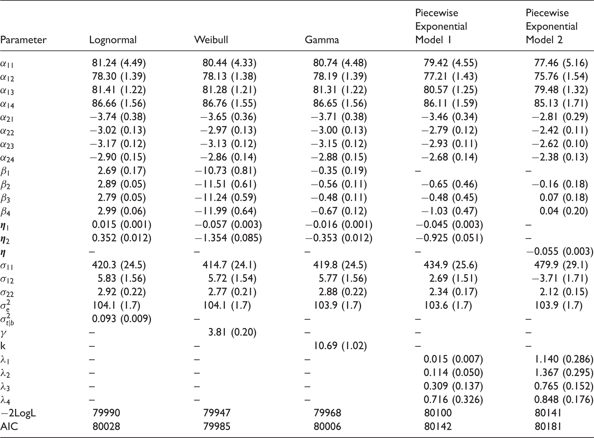
Results of fitting the lognormal and other models to the CF data are presented in Table 2. Estimates of

η_{1}

and

η_{2}

are both positive and highly statistically significant, indicating a strong relationship between survival (age at death) and mean %FEV₁ at age 6 as well as rate of decline in %FEV₁. For every increase of 1% predicted in %FEV₁ at age 6, or increase of 0.5 %predicted/year in slope of %FEV₁, survival times (including median age at death) increase by an estimated 100(exp(.015) − 1) = 1.5%, and 100(exp(0.5 × 0.352) − 1) = 19.2%, respectively. Estimated median ages at death for ‘average’ patients (having values of the random effects

b_{1 i}

and

b_{2 i}

equal to their population means of zero) in the four birth cohorts from earliest to latest, given by

exp (β_{g}) + 6

, for g = 1,…, 4 are 20.7, 24.0, 22.3, and 25.9, respectively. The null hypothesis that survival distributions do not differ among the four time periods

(H_{0} : β_{1} = β_{2} = β_{3} = β_{4})

is rejected using a Wald test with three degrees of freedom (p = 0.049).

Table 2.

Parameter estimates (SE’s) for models fit to CF data.

Parameter	Lognormal	Weibull	Gamma	Piecewise Exponential Model 1	Piecewise Exponential Model 2
$α_{11}$	81.24 (4.49)	80.44 (4.33)	80.74 (4.48)	79.42 (4.55)	77.46 (5.16)
$α_{12}$	78.30 (1.39)	78.13 (1.38)	78.19 (1.39)	77.21 (1.43)	75.76 (1.54)
$α_{13}$	81.41 (1.22)	81.28 (1.21)	81.31 (1.22)	80.57 (1.25)	79.48 (1.32)
$α_{14}$	86.66 (1.56)	86.76 (1.55)	86.65 (1.56)	86.11 (1.59)	85.13 (1.71)
$α_{21}$	−3.74 (0.38)	−3.65 (0.36)	−3.71 (0.38)	−3.46 (0.34)	−2.81 (0.29)
$α_{22}$	−3.02 (0.13)	−2.97 (0.13)	−3.00 (0.13)	−2.79 (0.12)	−2.42 (0.11)
$α_{23}$	−3.17 (0.12)	−3.13 (0.12)	−3.15 (0.12)	−2.93 (0.11)	−2.62 (0.10)
$α_{24}$	−2.90 (0.15)	−2.86 (0.14)	−2.88 (0.15)	−2.68 (0.14)	−2.38 (0.13)
$β_{1}$	2.69 (0.17)	−10.73 (0.81)	−0.35 (0.19)	–	–
$β_{2}$	2.89 (0.05)	−11.51 (0.61)	−0.56 (0.11)	−0.65 (0.46)	−0.16 (0.18)
$β_{3}$	2.79 (0.05)	−11.24 (0.59)	−0.48 (0.11)	−0.48 (0.45)	0.07 (0.18)
$β_{4}$	2.99 (0.06)	−11.99 (0.64)	−0.67 (0.12)	−1.03 (0.47)	0.04 (0.20)
$η_{1}$	0.015 (0.001)	−0.057 (0.003)	−0.016 (0.001)	−0.045 (0.003)	–
$η_{2}$	0.352 (0.012)	−1.354 (0.085)	−0.353 (0.012)	−0.925 (0.051)	–
η	–	–	–	–	−0.055 (0.003)
$σ_{11}$	420.3 (24.5)	414.7 (24.1)	419.8 (24.5)	434.9 (25.6)	479.9 (29.1)
$σ_{12}$	5.83 (1.56)	5.72 (1.54)	5.77 (1.56)	2.69 (1.51)	−3.71 (1.71)
$σ_{22}$	2.92 (0.22)	2.77 (0.21)	2.88 (0.22)	2.34 (0.17)	2.12 (0.15)
$σ_{e}^{2}$	104.1 (1.7)	104.1 (1.7)	103.9 (1.7)	103.6 (1.7)	103.9 (1.7)
$σ_{t \| b}^{2}$	0.093 (0.009)	–	–	–	–
γ	–	3.81 (0.20)	–	–	–
k	–	–	10.69 (1.02)	–	–
$λ_{1}$	–	–	–	0.015 (0.007)	1.140 (0.286)
$λ_{2}$	–	–	–	0.114 (0.050)	1.367 (0.295)
$λ_{3}$	–	–	–	0.309 (0.137)	0.765 (0.152)
$λ_{4}$	–	–	–	0.716 (0.326)	0.848 (0.176)
−2LogL	79990	79947	79968	80100	80141
AIC	80028	79985	80006	80142	80181

4.2 Weibull model

A Weibull proportional hazards model where the scale parameter is a function of the fixed effects covariates and random effects $b_{i}$ is specified by writing the conditional hazard function as

λ_{t | b} (t | b_{i}) = λ_{0} (w_{i}, b_{i}) γ t^{γ - 1}

where γ is a shape parameter, and

\begin{matrix} λ_{0} (w_{i}, b_{i}) = exp (w'_{i} β + η' b_{i}) = exp (G_{1 i} β_{1} + \dots + G_{4 i} β_{4} + η_{1} b_{1 i} + η_{2} b_{2 i}) \end{matrix}

(10)

for the CF data. Here, the hazard ratio comparing subjects in birth cohorts k vs l, conditional on subjects having similar random effects, is

e^{β_{k} - β_{l}}

, and

e^{η_{1}}

and

e^{η_{2}}

are hazard ratios corresponding to a 1-unit increase in the random intercept and slope, respectively. In addition to being a proportional hazards model, the Weibull model is the only parametric model that can be represented both a PH and an AFT model.⁵ To see this, the logarithm of survival time can be written as

\begin{matrix} log (T_{i}^{0}) = - γ^{- 1} log (λ_{0} (w_{i}, b_{i})) + γ^{- 1} ɛ_{i} = G_{1 i} β_{1}^{*} + \dots + G_{4 i} β_{4}^{*} +_{η_{1}}^{*} b_{1 i} + η_{2}^{*} b_{2 i} + γ^{- 1} ɛ_{i} \end{matrix}

where

ɛ_{i}

has the extreme value density

f (ɛ_{i}) = exp (ɛ - e^{ɛ})

β_{g}^{*} = - β_{g} / γ

, and

η_{k}^{*} = - η_{k} / γ

for g = 1,…,4 and k = 1,2. If

\hat{β}

and

\hat{η}

along with

\hat{γ}

are estimates of regression coefficients and the shape parameter in the Weibull PH model, the corresponding regression coefficients in the Weibull AFT model are

{\hat{β}}^{*} = - \hat{β} / \hat{γ}

and

{\hat{η}}^{*} = - \hat{η} / \hat{γ}

Conditional on $b_{i}$ , the survival function and density of $T_{i}^{0}$ , respectively, are $S_{t | b} (t | b_{i}; θ) = exp (- e^{w'_{i} β + η' b_{i}} t^{γ})$ and $π_{t | b} (t) = λ_{t | b} (t | b_{i}) S_{t | b} (t | b_{i})$ , where $θ' = (β', η', γ)$ . In calculating the log likelihood for a subject with left truncation time L_i > 0 (equation (6)), $S_{t} (L_{i})$ depends on $b_{i}$ only through the term $x_{i} = w'_{i} β + η' b_{i}$ , where $S_{t} (L_{i}) = E_{x} {exp (- L_{i}^{γ} e^{x_{i}})}$ , i.e. is the expectation of the function $g (x_{i}) = exp (- L_{i}^{γ} e^{x_{i}})$ , where $x_{i} \sim N (μ_{x}, σ_{x}^{2}),$ with $μ_{x} = w'_{i} β$ and $σ_{x}^{2} = η_{1}^{2} σ_{11} + 2 η_{1} η_{2} σ_{12} + η_{2}^{2} σ_{22}$ . While there is no closed-form expression for this term, it can be calculated using numerical integration, programmed within the user-supplied PROC NLMIXED code. We do this using Gauss–Hermite quadrature (see Appendix 1).

4.2.1 Results – Weibull Model

Estimated intercepts and slopes of %FEV₁ obtained fitting the Weibull model (Table 2) are very similar to those from the lognormal model. The random intercept and slope both have highly significant effects on survival, as indicated by the estimates of ${\hat{η}}_{1}$ and ${\hat{η}}_{2}$ and their standard errors. For every increase of 1% in %FEV₁ at age 6, or increase in 0.5% predicted/year in slope of %FEV₁, the hazard is estimated to decrease by the factor exp(−0.057) = 0.944 and exp(−0.5 × 1.354) = 0.508, i.e. by 5.6% and 49.2%, respectively. Alternatively, coefficients of the random intercept and slope in the Weibull AFT model are 0.057/3.81 = 0.015 and 1.354/3.81 = 0.355, which are equal or very close to, and have the same interpretation as, the regression coefficients obtained from the lognormal model. Estimated median survival times in the four birth cohorts are 21.2, 24.7, 23.4, and 27.1 years, respectively, qualitatively similar to the estimates from the lognormal model. Judging by AIC values, the Weibull model fits the CF data better than the lognormal model.

4.3 Gamma model

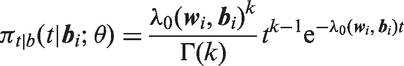
In the gamma AFT model, conditional on $b_{i}$ , the distribution of $T_{i}^{0}$ is assumed to have the gamma distribution

π_{t | b} (t | b_{i}; θ) = \frac{λ_{0} (w_{i}, b_{i})^{k}}{Γ (k)} t^{k - 1} e^{- λ_{0} (w_{i}, b_{i}) t}

where k > 0 is a shape parameter and

λ_{0} (w_{i}, b_{i})

is a scale parameter depending on the fixed and random effects as defined in equation (10). Under this model

log (T_{i}^{0}) = - (β_{1} G_{1} + \dots + β_{4} G_{4} + η_{1} b_{1 i} +_{2} b_{2 i}) + ɛ_{i}

where

ɛ_{i}

has distribution,

f (ɛ) = Γ (k)^{- 1} exp (k ɛ - e^{ɛ}) .

Interpretation of the elements of

β

and

η

is in terms of multiplicative effects on the distribution of survival times, analogous to the lognormal model, except that the signs of the regression coefficients are reversed. For example, an increase in 1 unit in the random effect

b_{2 i}

is associated with a change in survival times of

exp (- η_{2})

, where survival times are increased (decreased) if

η_{2}

is <(>) zero. Calculation of the term

S_{t} (L_{i})

in the likelihood is accomplished inside the NLMIXED program using numerical integration programmed by the user, as was done for the Weibull, utilizing the available GAMMA and CDF functions in SAS (see code in Supplemental Materials).

4.3.1 Results – Gamma model

Results of the Gamma model are shown in Table 2. Estimates of mean slopes and intercepts are similar to those obtained in the other models. According to the AIC, the fit of the Gamma model is better than that of the lognormal model, but not as good as the fit of the Weibull model. The negatives of the estimates of $η_{1}$ and $η_{2}$ from the Gamma model are very close to comparable estimates obtained in the lognormal and Weibull AFT models.

4.4 Piecewise Exponential Model 1 – random intercept and slope as predictors

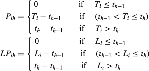
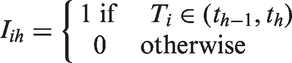
A piecewise exponential (PE) proportional hazards model can be used to approximate a baseline hazard function having an arbitrary shape. The follow-up time scale is divided into H intervals $(t_{h - 1}, t_{h}]$ , where $t_{0} = 0, t_{H} = \infty$ and the baseline hazard is defined to be a constant $λ_{h}$ in interval h, $h = 1, \dots,, H$ , i.e.

λ_{0} (t) = \sum_{h = 1}^{H} λ_{h} I (t \in (t_{h - 1}, t_{h}]

(11)

where

t_{0} = 0, t_{H} = \infty

, and

I (t \in (t_{h - 1}, t_{h}])

is 1 when

t_{h - 1} < h \leq t_{h}

and is zero otherwise. By defining a sufficiently large number of intervals, a hazard function with arbitrary shape can be approximated. A proportional hazards model where the hazard depends linearly on elements of

b_{i}

, with piecewise linear baseline hazard function, is specified by writing the conditional hazard function as:

λ_{t | b} (T_{i}^{0} = t_{i} | b_{i}) = λ_{0} (t) e^{w'_{i} β + η' b_{i}}

with

λ_{0} (t)

as in equation (11), and where for the CF data

exp (w'_{i} β + η' b_{i})

is given by equation (10). To avoid over-parameterization, we set

β_{1} = 0

in this model, where

β_{g}

is the log hazard ratio comparing birth cohort g to the first birth cohort, for g = 2,…,4.

To calculate the likelihood, define the following variables for each subject

\begin{matrix} P_{i h} = {\begin{array}{l} 0 & if T_{i} \leq t_{h - 1} \\ T_{i} - t_{h - 1} & if (t_{h - 1} < T_{i} \leq t_{h}) \\ t_{h} - t_{h - 1} & if T_{i} > t_{h} \end{array} \\ L P_{i h} = {\begin{array}{l} 0 & if L_{i} \leq t_{h - 1} \\ L_{i} - t_{h - 1} & if (t_{h - 1} < L_{i} \leq t_{h}) \\ t_{h} - t_{h - 1} & if L_{i} > t_{h} \end{array} \end{matrix}

and

I_{ih} = {\begin{matrix} 1 if T_{i} \in (t_{h - 1}, t_{h}) \\ 0 otherwise \end{matrix}

$P_{ih}$ and ${LP}_{ih}$ , respectively, are the amounts of person time in time interval h below T_i and L_i for a subject followed since time 0, for h = 1,…,H and i = 1,…,n.

For the CF data, we chose H = 4 time intervals for the piecewise exponential model: (6,15], (15,25], (25,35], and >35 years of age. These intervals were chosen to allow examination of changes in hazard across childhood, adolescence, and mid-adulthood, ensuring that there were nonzero numbers of deaths in each time interval and birth cohort. We did not fit models with different choices of time intervals; however, fit statistics such as AIC could be used to choose between models with different numbers and choices of intervals. Because in modeling the CF data the scale of $T_{i}^{0}$ is age minus six, the cutpoints in terms of $T_{i}^{0}$ are t₀ = 0, t₁ = 9, t₂ = 19, t₃ = 29, and t₄ = ∞.

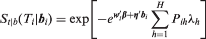
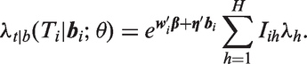
The likelihood for the piecewise exponential model is

\begin{matrix} l_{i} (α, σ_{e}^{2}, Σ, θ; y_{i}, T_{i}, δ_{i}, L_{i}, I_{i}^{tr}) = S_{t} (L_{i})^{- I_{i}^{tr}} \int_{b_{i}} π_{y | b} (y_{i} | b_{i}; α, σ_{e}^{2}) λ_{t | b} (T_{i} | b_{i}; θ)^{δ_{i}} S_{t | b} (T_{i} | b_{i}; θ) π (b_{i}; Σ) \partial b_{i} \end{matrix}

where

S_{t | b} (T_{i} | b_{i}) = exp [- e^{w'_{i} β + η' b_{i}} \sum_{h = 1}^{H} P_{ih} λ_{h}]

and

λ_{t | b} (T_{i} | b_{i}; θ) = e^{w_{i}' β + η' b_{i}} \sum_{h = 1}^{H} I_{ih} λ_{h} .

As for the Weibull and Gamma models, the conditional survival function $S_{t | b} (T_{i} | b_{i})$ depends on $b_{i}$ only through the linear combination $x_{i} = w_{i}' β + η_{1} b_{i 1} + η_{2} b_{i 1}$ which is normally distributed with mean $x_{i} = w_{i}' β$ and variance $σ_{x}^{2} = η_{1}^{2} σ_{11} + 2 η_{1} η_{2} σ_{12} + η_{2}^{2} σ_{22}$ . Computation of $S_{t} (L_{i})$ using Gaussian quadrature is carried out as described in Appendix 1.

4.4.1 Results – Piecewise Exponential Model 1

Results of PE Model 1 are shown in Table 2. Judging by its AIC, it does not fit the CF data as well as the Lognormal, Weibull, and Gamma models. Although it provides very similar estimates of the mean intercepts of %FEV₁, the estimates of %FEV₁ slope are somewhat less negative compared to estimates from the other models. The estimates of the baseline hazard rates: ${\hat{λ}}_{1} = 0.015,$ ${\hat{λ}}_{2} = 0.114,$ ${\hat{λ}}_{3} = 0.309,$ and ${\hat{λ}}_{4} = 0.716,$ indicate that the baseline hazard increases with age. The regression coefficients $η_{1}$ and $η_{2}$ in PE Model 1 have the same interpretation as they do in the Weibull model. Estimates of $η_{1}$ and $η_{2}$ obtained with the PE model (−0.045 and −0.925, respectively) are smaller in absolute magnitude than corresponding estimates obtained with the Weibull model (−0.057 and −1.354, respectively).

4.5 Piecewise Exponential Model 2 – time-dependent covariate

For the piecewise exponential model 2 with covariates that are time-dependent, the H time intervals are defined as previously, i.e. where interval h is $(t_{h - 1}, t_{h}]$ , for h = 1,…,H with $t_{0} = 0$ and $t_{H} = \infty$ , and baseline hazard function $λ_{0} (t)$ is as previously defined (equation (11)). As in Vonesh et al.,¹⁵ we consider a model where the time-varying covariate for survival is defined to be the subject’s true value of y at the beginning of the current time interval h, denoted as

\begin{matrix} μ_{i} (t_{h - 1}) = (α_{11} G_{1 i} + \dots + α_{14} G_{4 i} + b_{1 i}) + (α_{21} G_{1 i} + \dots + α_{24} G_{4 i} + b_{2 i}) t_{h - 1} \end{matrix}

and the conditional hazard function is

λ_{t | b} (T_{i}^{0} = t_{i} | b_{i}) = \sum_{h = 1}^{H} I_{ih} λ_{h} exp (w'_{i} β + η μ_{i} (t_{h - 1}))

The values of the $t_{h - 1}$ used in calculating $μ_{i} (t_{h - 1})$ are 0, 15 − 6 = 11, 25 − 6 = 19, and 35 − 6 = 29 for h = 1,…,4. The parameter η represents the change in the log hazard that results from an increase in 1 unit in the mean of y at the beginning of the current time interval. The conditional survival function used in computing the likelihood is

S_{t | b} (T_{i}^{0} = t | b_{i}; θ) = exp [- \sum_{h = 1}^{H} P_{ih} λ_{h} exp (w'_{i} β + η μ_{i} (t_{h - 1})]

and the term

S_{t} (L_{i})

is the expectation of

S_{t | b} (L_{i} | b_{i}; θ)

, with respect to

b_{i}

. Calculation of

S_{t} (L_{i})

using Gaussian quadrature by numerically integrating over both

b_{1 i}

and

b_{2 i}

is described in Appendix 1.

4.5.1 Results – Piecewise Exponential Model 2

Results of fitting this model are shown in Table 2. Compared to the piecewise exponential model 1 with no time-varying covariates, mean %FEV₁ intercepts are lower for the first two birth cohorts, and estimates of mean slopes are less negative. Based on the AIC criterion, PE model 2 has worse fit as compared to PE Model 1. Both PE models have higher AIC and poorer fit compared to the Weibull, Lognormal, and Gamma models. In PE Model 2, the estimated coefficient $\hat{η} = - 0.055$ indicates that for every 1% increase in current %FEV₁, the hazard of death is reduced by 100(1-exp(−.055)) = 5.4%, an effect comparable to the effects of the random %FEV₁ intercept at age six seen in the Weibull model and PE Model 1.

4.6 Estimation of marginal and subject-specific survival curves

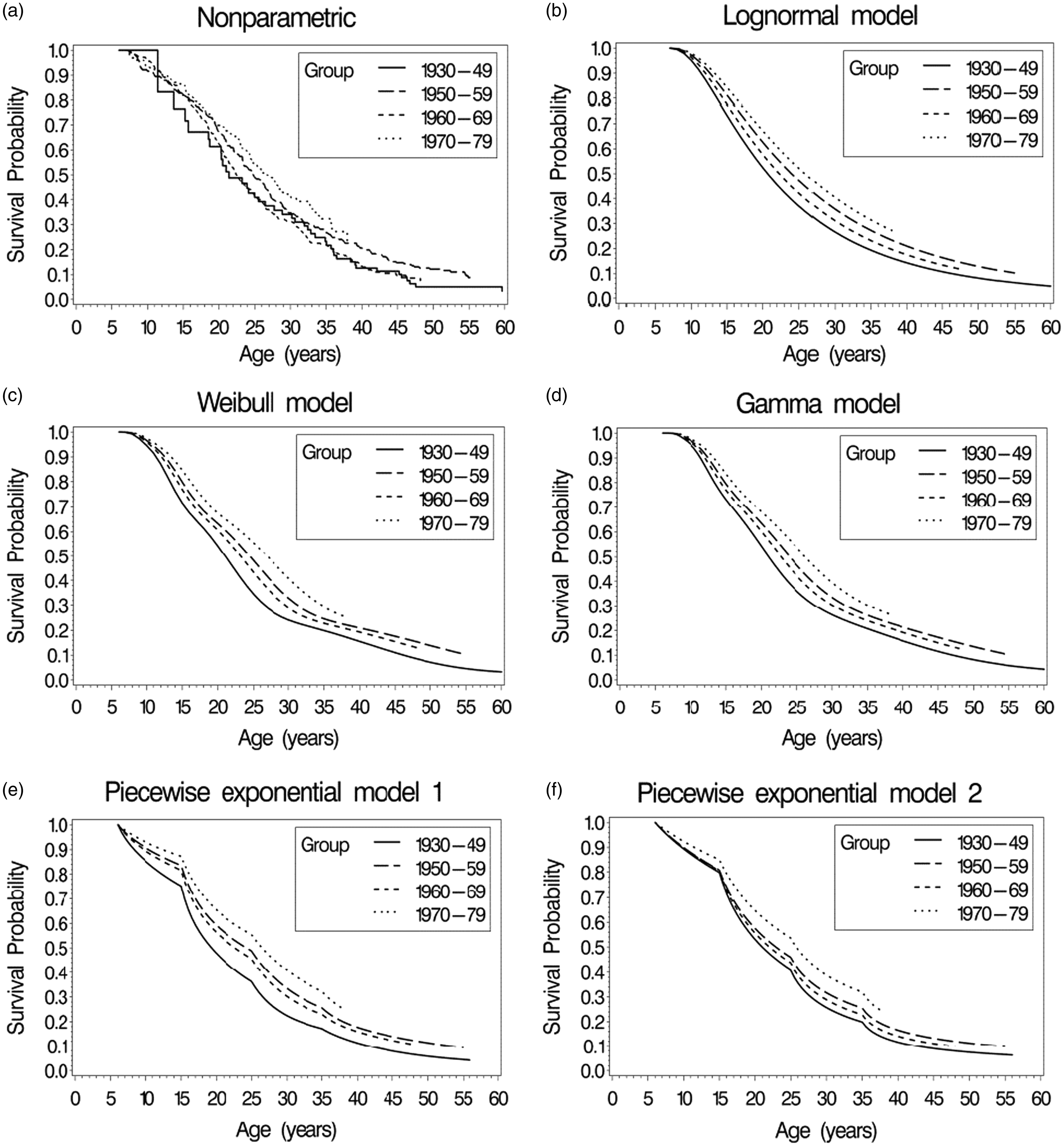
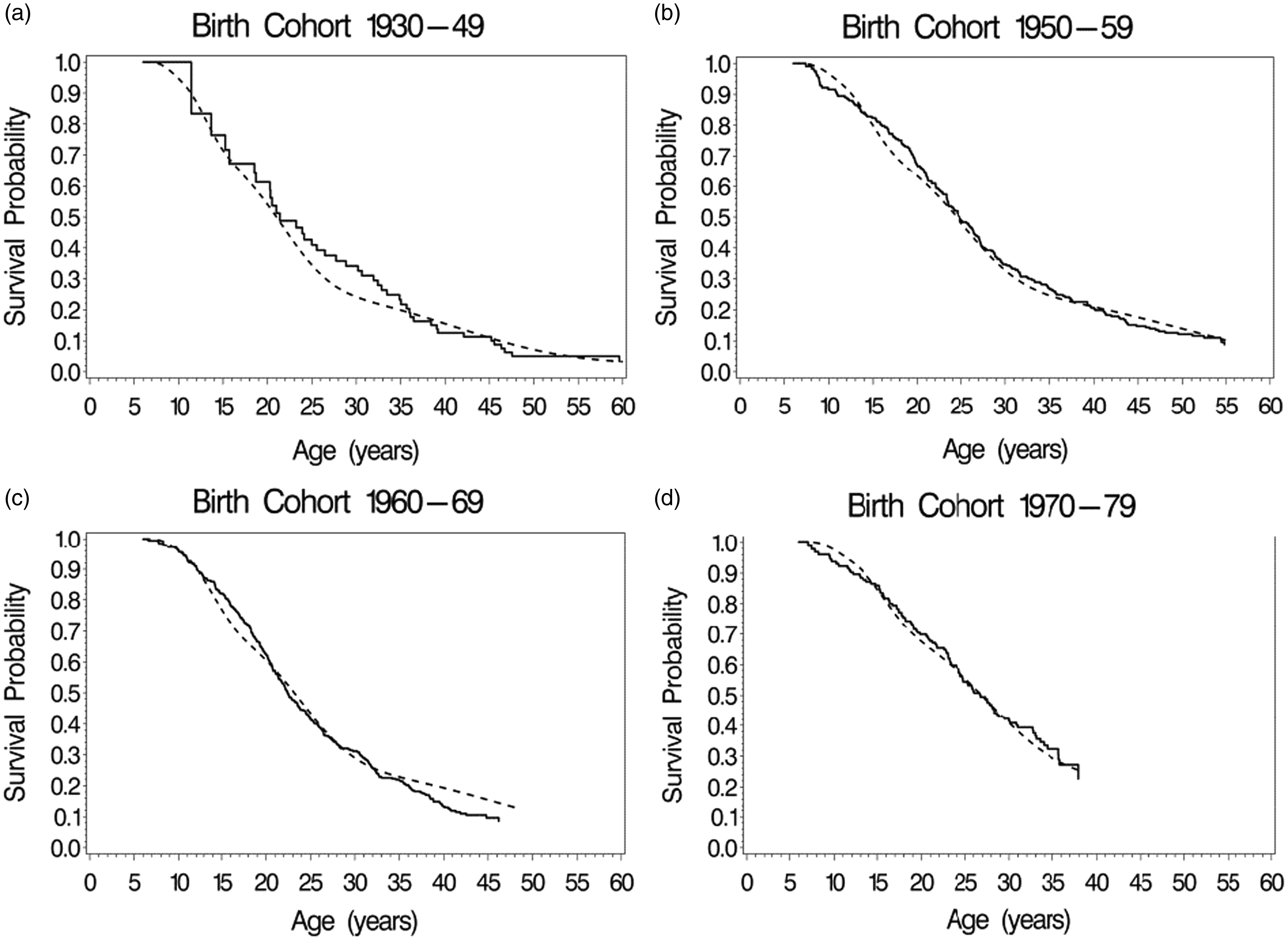
Estimates of the marginal or population-averaged survival curves for the four birth cohorts, $S_{t} (t)$ (equation (6)), are plotted in Figure 1 based on parameter estimates obtained from the five fitted models. Included in a separate panel of Figure 1 are nonparametric estimates of the survival curves for each cohort, obtained using the method = PL option for left truncated data in SAS PROC PHREG. The model-based and the non-parametric marginal survival estimates appear to be similar across models. For a more detailed comparison, Figure 2 plots the Weibull and non-parametric estimates together for each of the birth cohorts, demonstrating close agreement between the Weibull model-based and the non-parametric estimates.

Figure 1.

Estimates of marginal survival curves for the four birth cohorts in the cystic fibrosis data. (a) Nonparametric estimates accounting for left truncation, (b) Lognormal model, (c) Weibull model, (d) Gamma model, (e) piecewise exponential model 1, (f) piecewise exponential model 2.

Figure 2.

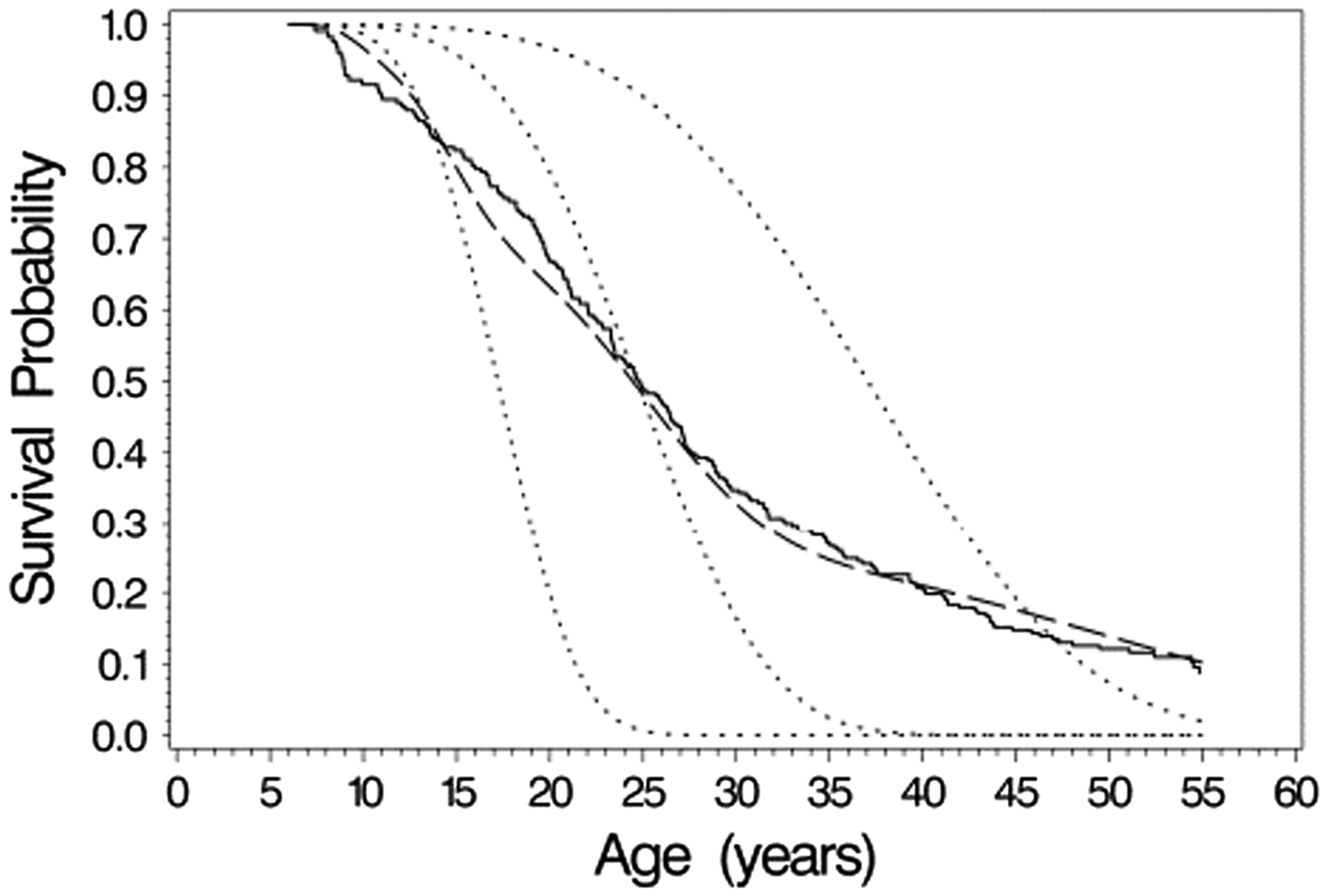
The marginal curves in Figures 1 and 2 estimate the population-averaged survival curves, which differ from subject-specific curves, i.e. plots of $S_{t | b} (t)$ conditional on the random effects. This is illustrated for the 1950–1959 birth cohort in Figure 3, which superimposes the marginal curve from the Weibull, the nonparametric (marginal) estimate, and conditional survival curves. Separate conditional survival curves are plotted corresponding to a subject with random intercept and slope $(b_{1 i}, b_{2 i})$ equal to the population mean (0,0), below normal $(b_{1 i} = - 10 %$ predicted, $b_{2 i} = - 0.5$ % predicted/year) and above normal $(b_{i 1} = 10$ % predicted, $b_{2 i} = 0.5$ % predicted/year). As was also noted by Vonesh et al. in the context of analyzing longitudinal measures of glomerular filtration rate (GFR) and time to end stage renal disease, the conditional survival curves differ markedly depending on the values of the intercept and slope, and differ in shape from the estimated marginal curves.¹⁵ For example, the estimated survival curve for subjects who are “average” in terms of their random slopes and intercepts ( $b_{i} = 0$ ) shows better survival initially compared to the marginal curve, but poorer survival at later ages.

Figure 3.

Comparison of survival curve estimates for the 1950–1959 birth cohort. Solid line: non-parametric estimate of marginal survival curve; Long dashed line: Weibull model estimate of marginal survival curve; short dashed lines are subject-specific survival curves from the Weibull model for subjects with random (intercept, slope) equal to (−10%, −0.5%/year), (0%, 0%/year), and (10%, 0.5%/year).

4.7 Comparison of hazard and average survival curve estimates among models

Figure 4(a) and (b) shows estimates of the conditional subject-specific hazard function and survival curve, respectively, obtained by fitting the lognormal, Weibull, gamma, and the two piecewise exponential models for the 1950–1959 birth cohort for a subject with average values of intercept and slope ( $b_{i} = 0$ ). Hazard plots for the other birth cohorts are similar in appearance except for shifts in the scales of the axes. All models indicate that the hazard is increasing with age, though the pattern of increase and shape of the curve differ. For the 1950–1959 birth cohort, the lognormal model estimate of the hazard increases and reaches a plateau with maximum at age 47 with a slight decline as age increases further. The gamma model estimate of hazard increases, with the rate of increase slowing at later ages. The Weibull hazard function on the other hand increases as a concave curve, suggesting a greater rate of increase at older ages. The piecewise exponential model estimates are similar to each other up to age 35, but diverge at ages >35 where model 2 (time-varying covariate) predicts a higher hazard than does model 1, and is more similar to the Weibull model than to the other models. Up to around age 25 the five models give similar estimates of hazard, but beyond age 35 the Weibull and PE models 1 and 2 predict higher risk than the lognormal and Gamma models do. Conditional survival curves when $b_{i} = 0$ for the Weibull, Lognormal, and gamma models are similar in shape, but the piecewise exponential models predict lower survival before age 23, but higher survival at ages 26–35.

Figure 4.

Estimated hazard function (a) and survival functions (b) from Lognormal, Weibull, Gamma, and piecewise exponential models for an average patient withrandom (intercept, slope)′ = (0,0)′ in the 1950–1959 birth cohort.

4.8 Examination of biases due to dropout caused by death and delayed entry

Analyzing the cystic fibrosis data using a joint modeling approach potentially reduces two sources of bias, as compared to separate analyses of the marker and survival, particularly with respect to parameters describing the longitudinal marker y. These are: (a) bias due to non-ignorable dropout, and (b) bias due caused by delayed entry or left-truncation of follow-up. To examine these potential biases, four models were fit using the Weibull model: (1) the joint model adjusting for left truncation (J-L), 2) the joint model not adjusting for left truncation (J-N), (3) separate (non-joint) models fit assuming survival and %FEV₁ are not correlated, but taking left truncation into account in the survival model (N-L), and (4) separate (non-joint) models fit where the left truncation is not taken into account in the survival model (N-N). All four models were fit using PROC NLMIXED; the non-joint models (N-L and N-N) were fit by restricting $η_{1}$ and $η_{2}$ to be zero, and left truncation was ignored by setting $L_{i} = 0$ and $I_{i}^{tr} = 0$ for all subjects in the input data. The non-joint models (N-L and N-N) assume that dropout due to death is an ignorable mechanism when analyzing the %FEV₁ data, and maximum likelihood estimates and standard errors for parameters of the distribution of %FEV₁ for these two models match the ML estimates obtained when the y data are separately analyzed using a mixed model program such as PROC MIXED in SAS. Also, the maximum likelihood estimates of the parameters of the survival distribution in the N-N model can be obtained using a parametric Weibull regression program such as PROC LIFEREG. However, PROC LIFEREG does not handle left-truncation in its parametric models so the N-L model cannot be fit using it.

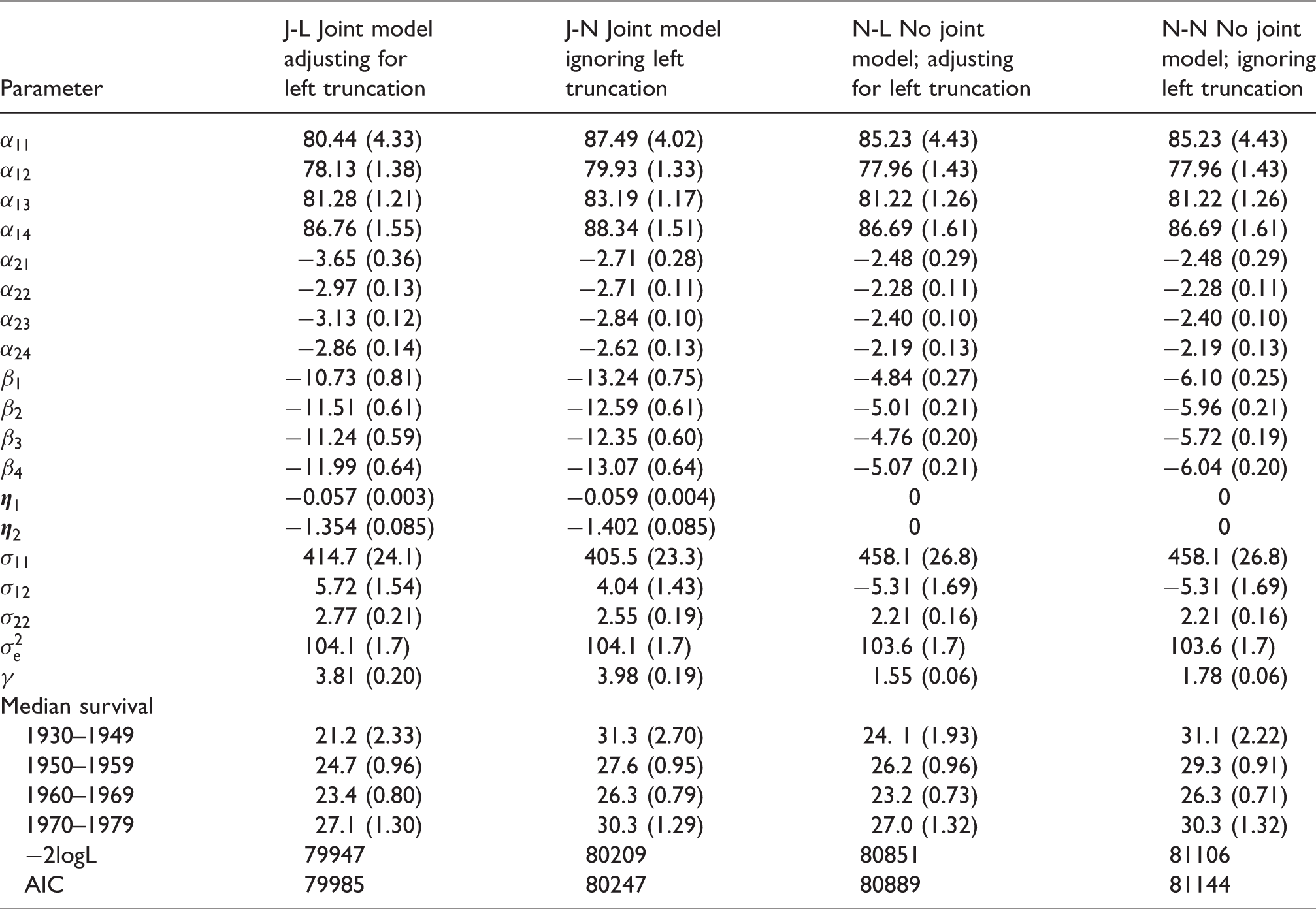
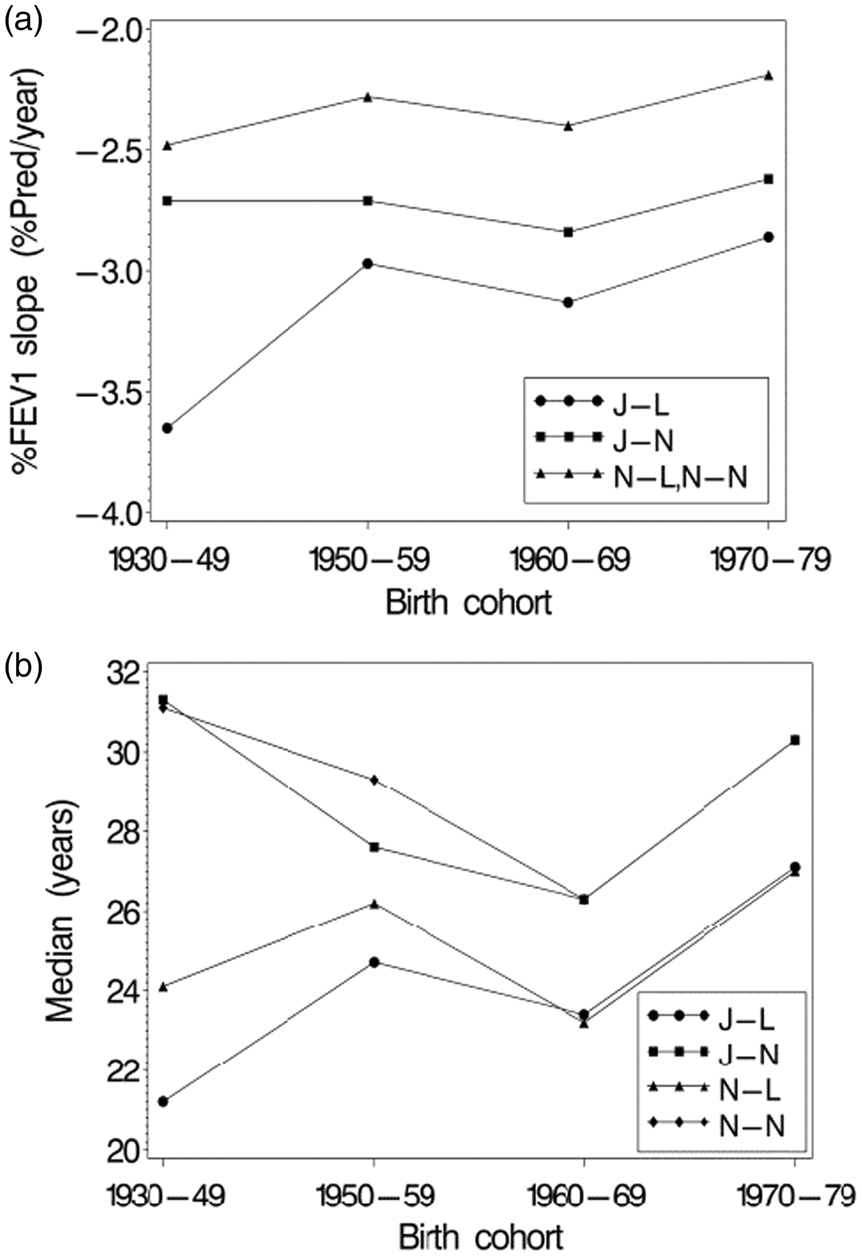
Results of fitting the four models are presented in Table 3. Estimated mean %FEV₁ slopes and median survival times for subjects with random effects values of

b_{1 i}

= 0 and

b_{2 i}

= 0 are presented in Figure 5(a) and (b), respectively. While log-likelihoods and AIC’s are presented in Table 3, likelihoods for the models that ignore left truncation (J-N and N-N) cannot be compared to those that incorporate the left truncation (J-L and N-L). For the oldest three birth cohorts, results for %FEV₁ slope (Figure 5(a)) consistently show that the joint model J-L, which corrects for both bias due to dropout and due to delayed entry, gives mean slope estimates that are more negative by 0.65–0.70% predicted per year, compared to the models ignoring the correlation between %FEV₁ and survival (N-N and N-L). In these cohorts, the slope estimates from the J-N model, which deals only with bias due to dropout but not due to delayed entry, are higher than the estimates from the J-L model by around 0.25% predicted per year, which quantifies the bias due only to ignoring effects of left truncation. For the 1930–1949 cohort, the difference in slopes between J-L and J-N models was larger, reflecting a potentially larger bias due to delayed entry, as was expected since of the four cohorts, the 1930–1949 cohort had the most extensive left truncation of follow-up.

Table 3.

Results of Weibull model fit with and without joint modeling and adjustment for left truncation.

Parameter	J-L Joint model adjusting for left truncation	J-N Joint model ignoring left truncation	N-L No joint model; adjusting for left truncation	N-N No joint model; ignoring left truncation
$α_{11}$	80.44 (4.33)	87.49 (4.02)	85.23 (4.43)	85.23 (4.43)
$α_{12}$	78.13 (1.38)	79.93 (1.33)	77.96 (1.43)	77.96 (1.43)
$α_{13}$	81.28 (1.21)	83.19 (1.17)	81.22 (1.26)	81.22 (1.26)
$α_{14}$	86.76 (1.55)	88.34 (1.51)	86.69 (1.61)	86.69 (1.61)
$α_{21}$	−3.65 (0.36)	−2.71 (0.28)	−2.48 (0.29)	−2.48 (0.29)
$α_{22}$	−2.97 (0.13)	−2.71 (0.11)	−2.28 (0.11)	−2.28 (0.11)
$α_{23}$	−3.13 (0.12)	−2.84 (0.10)	−2.40 (0.10)	−2.40 (0.10)
$α_{24}$	−2.86 (0.14)	−2.62 (0.13)	−2.19 (0.13)	−2.19 (0.13)
$β_{1}$	−10.73 (0.81)	−13.24 (0.75)	−4.84 (0.27)	−6.10 (0.25)
$β_{2}$	−11.51 (0.61)	−12.59 (0.61)	−5.01 (0.21)	−5.96 (0.21)
$β_{3}$	−11.24 (0.59)	−12.35 (0.60)	−4.76 (0.20)	−5.72 (0.19)
$β_{4}$	−11.99 (0.64)	−13.07 (0.64)	−5.07 (0.21)	−6.04 (0.20)
$η_{1}$	−0.057 (0.003)	−0.059 (0.004)	0	0
$η_{2}$	−1.354 (0.085)	−1.402 (0.085)	0	0
$σ_{11}$	414.7 (24.1)	405.5 (23.3)	458.1 (26.8)	458.1 (26.8)
$σ_{12}$	5.72 (1.54)	4.04 (1.43)	−5.31 (1.69)	−5.31 (1.69)
$σ_{22}$	2.77 (0.21)	2.55 (0.19)	2.21 (0.16)	2.21 (0.16)
$σ_{e}^{2}$	104.1 (1.7)	104.1 (1.7)	103.6 (1.7)	103.6 (1.7)
γ	3.81 (0.20)	3.98 (0.19)	1.55 (0.06)	1.78 (0.06)
Median survival
1930–1949	21.2 (2.33)	31.3 (2.70)	24. 1 (1.93)	31.1 (2.22)
1950–1959	24.7 (0.96)	27.6 (0.95)	26.2 (0.96)	29.3 (0.91)
1960–1969	23.4 (0.80)	26.3 (0.79)	23.2 (0.73)	26.3 (0.71)
1970–1979	27.1 (1.30)	30.3 (1.29)	27.0 (1.32)	30.3 (1.32)
−2logL	79947	80209	80851	81106
AIC	79985	80247	80889	81144

Figure 5.

Estimated mean slopes (a) and median survival times (b) by birth cohort based on Weibull models: J-L = Joint model accounting for left truncation, J-N = Joint model not accounting for left truncation, N-L = separate models accounting for left truncation in survival model, N-N = separate models not accounting for left truncation in survival model.

Estimates of median survival were consistently lower for models that accounted for left truncation (J-L, N-L) compared to models that did not (J-N, N-N), where the difference was around three years for the three older birth cohorts but was larger in the 1930–1949 cohort where left truncation was the most pronounced. There was relatively little difference between the J-L and N-L models, particularly in the older cohorts. This suggests that as long as left truncation is adjusted for in the survival model, using a joint model does not offer additional advantages in terms of bias reduction when estimating parameters of survival, at least in this dataset.

5 Assessing model fit and validity of assumptions

One method of assessing fit of survival model is illustrated in Figure 2, which compares the 1-slope Weibull model-estimated marginal survival curves to nonparametric estimates adjusting for left truncation, for each birth cohort. We now examine goodness of fit and validity of assumptions involving the linear mixed model for %FEV₁.

5.1 Examining non-linearity of trajectory of %FEV₁ vs. age

Previous papers analyzing data from adolescents and young adults with cystic fibrosis have found evidence for non-linearity in the %FEV₁ vs. age relationship, modeling nonlinearity using cubic splines²¹ or two-slope models with change points varying from 15 to 21 years of age.^22–24 As a sensitivity analysis, we fit 2-slope Weibull models with change point A₀, with the linear mixed model

\begin{matrix} y_{it} | b_{i} = (\sum_{g = 1}^{4} α_{1 g} G_{gi} + b_{1 i}) + (\sum_{g = 1}^{4} α_{2 g} G_{gi} + b_{2 i}) ({Age}_{it} - 6) + (\sum_{g = 1}^{4} α_{3 g} G_{gi}) ({Age}_{it} - A_{0})^{+} + e_{it} \end{matrix}

(12)

where

a^{+} = a

if a > 0, and is 0 otherwise. Models were fit varying A₀ from 15 to 28 years. Slopes before and after age A₀ are given by

α_{2 i}

and

α_{2 i} + α_{3 i}

, respectively. The model in equation (12) utilizes a technique used previously in modeling lung function decline, where a nonlinear (here 2-slope) regression is combined with a random intercept and slope model to account for between-subject variability.²⁵ Based on comparison of −2LogL values (Supplemental Figure S1), the models with A₀ equal to 25 and 26 fit equally well and the model with A₀ = 25 was arbitrarily selected as the best 2-slope model. Likelihood ratio tests indicated the 2-slope model with A₀ = 25 fits significantly better than the one slope model (p < 0.0001), and also fits better (p < 0.05) than 2-slope models with change point 15 ≤ A₀ ≤ 21.

Maximum likelihood estimates from the 2-slope model are shown in Supplemental Table S1. Estimates of all $α_{3 i}$ parameters were positive and differed significantly from zero, indicating a less steep average decline in %FEV₁ after age 25. Estimated mean trajectories $E (y_{it} | b_{i})$ for the 1- and 2-slope models (using equations 7 and 12, respectively) for the scenarios $(b_{1 i}, b_{i 2})' = (0, 0)'$ and $(b_{1 i}, b_{i 2})' = (0, 1)'$ are shown in Figure 6 for the 1950–1959 cohort, and in Supplemental Figure S2 for all cohorts. These plots indicate very similar mean trajectories for 1- and 2-slope models up to age 25, with some divergence after age 25. Other differences between results of 1- and 2-slope models were minor. Estimated median survival times in the 2-slope model for the four cohorts were 21.0, 24.7, 23.4, and 27.3 for cohorts 1930–1949, 1950–1959, 1960–1969, and 1970–1979, very close to the estimates in the one-slope model (21.2, 24.7, 23.4, 27.1, respectively). Weibull shape parameters were similar for one- and 2-slope models (3.81 and 3.67, respectively).

Figure 6.

Estimated mean trajectories for 1- and 2-slope Weibull models for the 1950–1959 birth cohort. Solid lines are for the 1-slope model, and dashed lines are for 2-slope model. Bolded lines are for a subject with random (intercept, slope) equal to (0,0), and unbolded lines are for a subject with random (intercept, slope) equal to (0,1).

5.2 Comparing marginal to model-predicted means, conditional on $T_{i}^{0} \geq t$

When there is association between $y_{it}$ and $T_{i}^{0}$ (i.e. when $η \neq 0$ ), observed values of $y_{it}$ plotted vs. time do not follow the marginal trajectory predicted by the fixed effects in the linear mixed model, due to survivor bias. Under the 1-slope model, the mean of %FEV₁ of subjects remaining alive at time t, can be written as

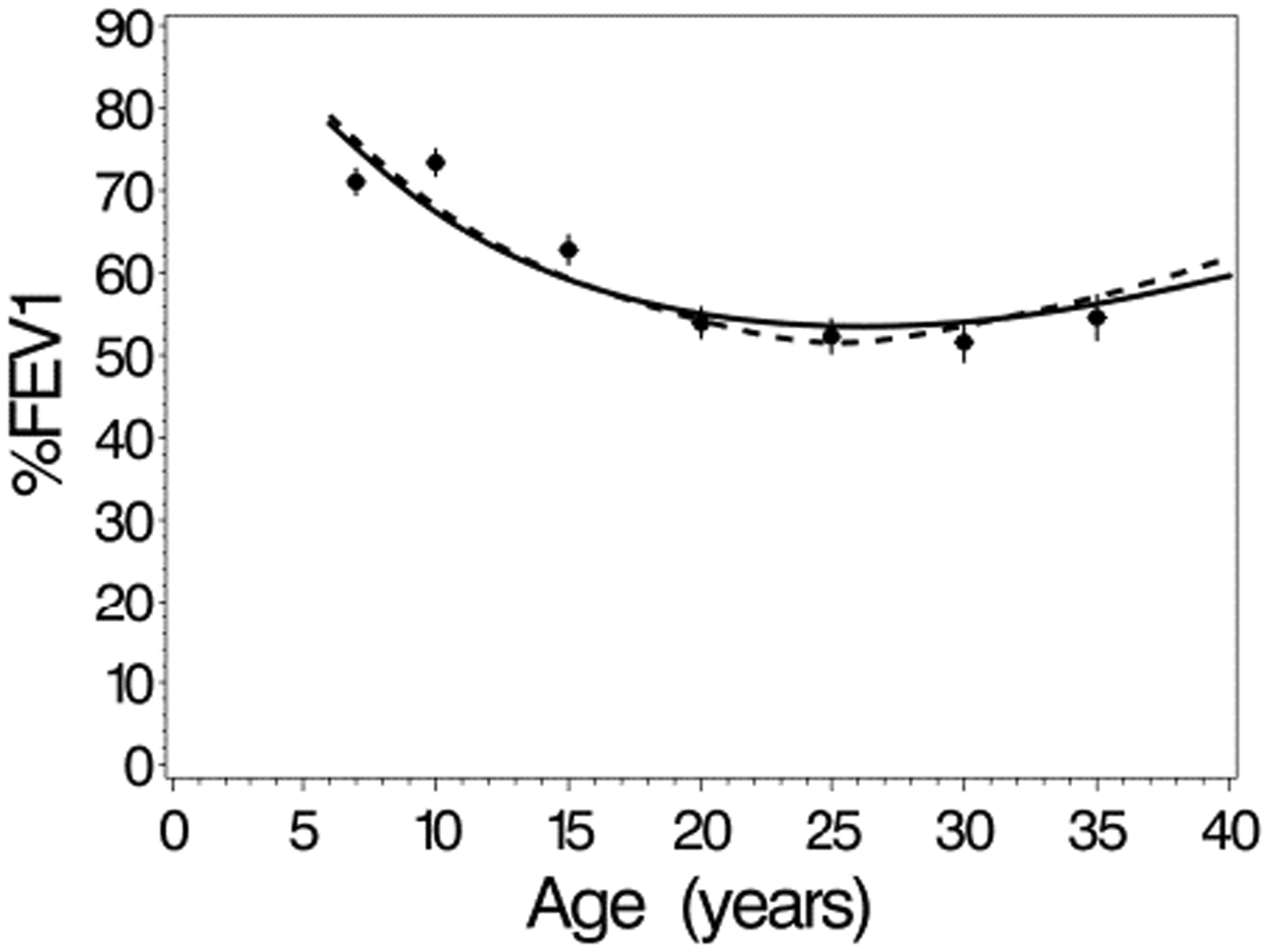
\begin{matrix} E (y_{it} | T_{i}^{0} \geq t) = (\sum_{g = 1}^{4} α_{1 g} G_{gi} + E (b_{1 i} | T_{i}^{0} \geq t)) + (\sum_{g = 1}^{4} α_{2 g} G_{gi} + E (b_{2 i} | T_{i}^{0} \geq t)) ({Age}_{it} - 6)^{+} \end{matrix}

The mean for the 2-slope model is the same, with $(\sum_{g = 1}^{4} α_{3 g} G_{gi}) ({Age}_{it} - A_{0})^{+}$ added to the right-hand side of the equation. One way to assess fit of the model is to compare “observed” vs. model-based estimates of these conditional means. To estimate $E (y_{it} | T_{i}^{0} \geq t)$ for a given t, we simulated values of $b_{i}$ and $T_{i}^{0}$ from their joint distribution under the 1- and 2-slope models, assuming the true parameters values were equal to the MLEs, repeating the simulation until 200,000 subjects with values of $T_{i}^{0} \geq t$ were obtained. Simulated mean values of $b_{1 i}$ and $b_{2 i}$ were used as estimates of $E (b_{1 i} | T_{i}^{0} \geq t)$ and $E (b_{2 i} | T_{i}^{0} \geq t)$ , respectively, allowing estimation of $E (y_{it} | T_{i}^{0} \geq t)$ . By varying t from 6 to 40 and fitting a spline smoother, we obtained marginal mean profiles of %FEV₁ for the four birth cohorts. Estimates of the observed mean %FEV₁ for each cohort at time t, t = 7, 10, 15, 20, … , 35 were obtained by fitting a linear mixed model with random intercept and slope, using only subjects alive at time t years, and restricting %FEV₁ data to the age interval (t, t + 5). Plots of observed and expected means from the 1- and 2-slope model, shown for the 1950–1959 cohort in Figure 7 and for all cohorts in Supplemental Figure S3 indicate reasonably good agreement between observed and model-predicted means, and with only minor differences in predicted marginal mean curves between the 1- and 2-slope models.

Figure 7.

Predicted and observed means of %FEV₁, conditional on surviving to a given age, for the 1950–59 birth cohort. Solid and dashed lines are the estimated conditional means obtained from the 1- and 2-slope Weibull models, respectively. Dots are the observed conditional means, obtained from a mixed model (see text). Error bars are plus or minus one standard error.

5.3 Analysis of conditional residuals

Analyses and plots of conditional residuals, ${\hat{e}}_{it} = y_{it} - \hat{E} (y_{it} | {\hat{b}}_{i})$ can be used to examine assumptions of normality, equal variance and conditional independence of residuals $e_{it}$ in the linear mixed model. Residuals ${\hat{e}}_{it}$ were calculated after obtaining $\hat{E} (y_{it} | {\hat{b}}_{i})$ using the Predict statement in PROC NLMIXED for both 1- and 2-slope Weibull models. Plots of the residuals vs. age and versus the predicted value $\hat{E} (y_{it} | {\hat{b}}_{i})$ (Supplemental Figure S4) appear as random scatters of points with little or only slight systematic trends, and appear similar for the 1- and 2-slope models. Residual variability, however, decreases somewhat with increasing age or decreasing predicted value. Histograms of the residuals (not shown) appear approximately normally distributed, although with somewhat heavier extreme tails.

To assess the assumption conditional independence of the residuals, i.e. that $var (e_{i}) = σ^{2} I_{i}$ , made when using PROC NLMIXED, we fit a mixed model to the estimated residuals ${\hat{e}}_{it}$ from the 1- and 2-slope models, with only a single intercept as fixed effect using SAS PROC MIXED, and assuming the SP(EXP) spatial exponential autocorrelation structure with age as the distance measure. This model assumes that the covariance between residuals $e_{it}$ and $e_{it'}$ corresponding to measures of %FEV₁ at ages $t_{it}$ and $t_{it'}$ is $cov (e_{it}, e_{it'}) = σ^{2} e^{- | t_{it} - t_{it'} | / τ}$ . The MLEs of τ were 0.50 (SE = 0.02) and 0.51 (SE = 0.02) for the 1- and 2-slope models. Estimated lag 1 and 2-year correlations were 0.14 and 0.02, respectively in both models, indicating statistically significant but relatively low degrees of autocorrelation. Note that our approach of analyzing maximal yearly %FEV₁ values, rather than all possible values is expected to reduce the degree of autocorrelation in the data by smoothing over short-term fluctuations in %FEV₁ caused, for example, by intercurrent illness.

6 Discussion

Shared parameter models provide a flexible approach for joint modeling, easily implemented using standard nonlinear mixed modeling software.^14–16 In this paper, we extend this flexible modeling approach to incorporate left-truncated observations, showing how they can be fit using SAS PROC NLMIXED. The extension requires the user to provide a relatively small amount of additional programming code to calculate a term required for the log-likelihood when there is left truncation, using Gaussian quadrature. The extension leverages the flexible nonlinear mixed modeling machinery already available in PROC NLMIXED to allow fitting a wide class of models.

This paper extends previous work fitting the lognormal AFT model to cystic fibrosis data using a novel EM algorithm.¹⁰ The approach described herein is more general, considering a broader class of models for $T_{i}^{0} | b_{i}$ , including Weibull, gamma, and piecewise exponential models. When fitting the lognormal model to the CF data, the EM algorithm¹⁰ and the approach described in this paper yield identical maximum likelihood estimates. Although our previous paper presented limited simulation studies examining performance of the lognormal joint model with left truncation under the assumed model and with model misspecification, further studies of the validity and robustness of these methods under more general conditions or where assumptions such as conditional independence of residuals are not met are warranted.

Analyses of the cystic fibrosis registry data using the Weibull model illustrate the importance of properly accounting for left truncation of follow-up times. We investigated the separate biases caused by non-ignorable dropout (i.e. death) and delayed entry (left truncation) by applying the Weibull model to the CF data. Joint model J-L appeared to correct for biases in mean estimates for %FEV₁ caused by non-ignorable dropout and delayed entry. This was also shown in previous simulation studies based on the lognormal AFT model.¹⁰ Based on these findings, we recommend the use of joint modeling with adjustment for left truncation to account for delayed entry when applicable. We also emphasize the importance of assessing, to the extent possible, the fit of these models and validity of assumptions using graphical and diagnostic techniques described in this paper and elsewhere.^3,15,25 The ability to fit and compare a broad variety of models to a given dataset using this proposed approach also provides another useful type of sensitivity analysis.

Our primary analysis of the cystic fibrosis data focused on fitting models assuming linear decline in %FEV₁ to illustrate the methodology, as done previously.¹⁰ In further sensitivity analyses, a 2-slope model for change in %FEV₁ was found to provide better fit, though actual predictions of mean trajectories of %FEV₁ and median survival of the 1- and 2-slope models were not very different. Our finding that the optimal change point for slope was at 25–26 years differs from results of analyses of other CF datasets where 2-slope models with change points between 15 and 21 years were fit.^22–24 In analyzing %FEV₁ decline using data from Danish CF registry, Taylor-Robinson²⁵ reported evidence supporting a 2-slope model with change point at 25 years; however, it did not significantly improve fit over a 1-slope model.

This paper focuses on the case where y is a continuous outcome where the distribution $y_{i} | b_{i}$ follows a linear mixed model with Gaussian errors, and the random effects $b_{i}$ have a multivariate normal distribution. Extensions to the case where y is a binary or count variable, using a generalized linear model to model $y_{i} | b_{i}$ are possible using the same software and approach. While this paper focused on simple linear trajectories for y given time, polynomials or restricted cubic splines could be used to provide flexible modeling of the mean of y vs. time, as in Crowther et al.,⁸ and as used by Szczesniak et al.²¹ in modeling %FEV₁ decline in cystic fibrosis.

We used piecewise exponential models (PE models 1 and 2) as a way to flexibly model an arbitrary baseline hazard function. In PE model 1, the hazard depends on subject random effects directly through $b_{i}$ in a time-invariant way, whereas in PE model 2, the hazard at time t is a function of a subject’s mean of y at time t, conditional on $b_{i}$ , i.e. as a time-varying covariate. A possible alternative approach to piecewise exponential models is to model the baseline log hazard function using restricted cubic splines. This approach was taken by Crowther et al.,⁸ who considered models where the effect of $b_{i}$ on the hazard was through the current mean of y, $μ_{i} (t)$ as in our PE model 2, through the current rate of change in y, $μ'_{i} (t)$ , as well as models where the hazard depends on the $b_{i}$ in a non-time-varying way.

Supplemental Material

Supplemental material SAS Code -Supplemental material for Shared parameter models for joint analysis of longitudinal and survival data with left truncation due to delayed entry – Applications to cystic fibrosis

Supplemental material, Supplemental material SAS Code for Shared parameter models for joint analysis of longitudinal and survival data with left truncation due to delayed entry – Applications to cystic fibrosis by Mark D Schluchter and Annalisa V Piccorelli in Statistical Methods in Medical Research

Supplemental Material

Supplementary Tables and Figures -Supplemental material for Shared parameter models for joint analysis of longitudinal and survival data with left truncation due to delayed entry – Applications to cystic fibrosis

Supplemental material, Supplementary Tables and Figures for Shared parameter models for joint analysis of longitudinal and survival data with left truncation due to delayed entry – Applications to cystic fibrosis by Mark D Schluchter and Annalisa V Piccorelli in Statistical Methods in Medical Research

Footnotes

Declaration of conflicting interests

The author(s) declared no potential conflicts of interest with respect to the research, authorship, and/or publication of this article.

Funding

The author(s) disclosed receipt of the following financial support for the research, authorship, and/or publication of this article: This research was supported in part by NIH grant P30 DK027651.

Supplemental material

Supplemental material for this article is available online.

Appendix 1. Computing the term S t (L i )

References

Gould

Boye

Crowther

et al.

Joint modeling of survival and longitudinal non-survival data: current methods and issues. Report of the DIA Bayesian joint modeling working group. Stat Med 2015; 34: 2181–2195.

Tsiatis

Davidian

. Joint modeling of longitudinal and time-to-event data: an overview. Stat Sinica 2004; 14: 809–834.

Rizopoulos

. Joint models for longitudinal and time-to-event data with applications in R, New York, NY: Chapman & Hall, 2012.

Sudell

Kolamunnage-Dona

Tudur-Smith

. Joint models for longitudinal and time-to-event data: a review of reporting quality with a view to meta-analysis. BMC Med Res Methodol 2016; 16: 168–168.

Klein

Moeschberger

. Survival analysis – techniques for censored and truncated data, 2nd ed. New York: Springer, 2003, pp. 536–536.

Tsai

Jewell

Wang

. A note on the product-limit estimator under right censoring and left truncation. Biometrica 1987; 74: 883–886.

Woodroofe

. Estimating a distribution function with truncated data. Ann Stat 1985; 13: 163–177.

Crowther

Andersson

TML

Lambert

et al.

Joint modelling of longitudinal and survival data: incorporating delayed entry and an assessment of model misspecification. Stat Med 2016; 35: 1193–1209.

Dantan

Joly

Dartigues

et al.

Joint model with latent state for longitudinal and multistate data. Biostatistics 2011; 12: 723–736.

10.

Piccorelli

Schluchter

. Jointly modeling the relationship between longitudinal and survival data subject to left truncation with applications to cystic fibrosis. Stat Med 2012; 31: 3931–3945.

11.

Proust-Lima

Joly

Dartigues

et al.

Joint modelling of multivariate longitudinal outcomes and a time-to-event: a nonlinear latent class approach. Computat Stat Data Analysis 2009; 53: 1142–1154.

12.

van den Hout

Muniz-Terrera

. Joint models for discrete longitudinal outcomes in aging research. Appl Stat 2016; 65: 167–186.

13.

Crowther

Abrams

Lambert

. Joint modeling of longitudinal and survival data. Stata J 2013; 13: 165–184.

14.

Guo

Carlin

. Separate and joint modeling of longitudinal and event time data using standard computer packages. Am Stat 2004; 58: 16–24.

15.

Vonesh

Greene

Schluchter

. Shared parameter models for the joint analysis of longitudinal data and event times. Stat Med 2006; 25: 143–163.

16.

Wang

Mosley

et al.

A SAS macro for the joint modeling of longitudinal outcomes and multiple competing risk dropouts. Comput Meth Program Biomed Res 2017; 138: 23–30.

17.

Schluchter

Konstan

Davis

. Jointly modeling the relationship between survival and FEV1 in cystic fibrosis patients. Stat Med 2002; 21: 1271–1287.

18.

Schluchter

Konstan

Drumm

et al.

Classifying severity of cystic fibrosis lung disease using longitudinal pulmonary function data. Am J Respirat Crit Care Med 2006; 174: 780–786.

19.

Schluchter

. Methods for the analysis of informatively censored longitudinal data. Stat Med 1992; 11: 1861–1870.

20.

Schluchter

Greene

Beck

. Analysis of change in the presence of informative censoring – application to a longitudinal clinical trial of progressive renal disease. Stat Med 2001; 20: 989–1007.

21.

Szczesniak

McPhail

Duan

et al.

A semiparametric approach to estimate rapid lung function decline in cystic fibrosis. Ann Epidemiol 2013; 23: 771–777.

22.

Dasenbrook

Merlo

Diener-West

et al.

Persistent methicillin-resistant Staphylococcus aureus and rate of FEV1 decline in cystic fibrosis. Am J Respir Crit Care Med 2008; 178: 814–821.

23.

Moss

Juarez-Colunga

Nathoo

et al.

A comparison of change point models with application to longitudinal lung function measurements in children with cystic fibrosis. Stat Med 2016; 35: 2058–2073.

24.

Vandenbranden

McMullen

Schechter

et al.

Lung function decline from adolescence to young adulthood in cystic fibrosis. Pediatric Pulmonol 2012; 47: 135–143.

25.

Taylor-Robinson

Whitehead

Diderichsen

et al.

Understanding the natural progression in %FEV1 decline in patients with cystic fibrosis: a longitudinal study. Thorax 2012; 67: 860–866.

26.

Abramowitz

Stegun

. Handbook of mathematical functions with formulas, graphs, and mathematical tables, New York, NY: Dover, 1964.

Supplementary Material

Please find the following supplemental material available below.

For Open Access articles published under a Creative Commons License, all supplemental material carries the same license as the article it is associated with.

For non-Open Access articles published, all supplemental material carries a non-exclusive license, and permission requests for re-use of supplemental material or any part of supplemental material shall be sent directly to the copyright owner as specified in the copyright notice associated with the article.

0.00 MB

0.23 MB

0.31 MB

Shared parameter models for joint analysis of longitudinal and survival data with left truncation due to delayed entry – Applications to cystic fibrosis

Abstract

Keywords

1 Introduction

2 Model and notation

3 Maximum likelihood estimation of parameters

4 Application to analysis of cystic fibrosis data

4.1 Lognormal model

4.1.1 Results – Lognormal model

4.2 Weibull model

4.2.1 Results – Weibull Model

4.3 Gamma model

4.3.1 Results – Gamma model

4.4 Piecewise Exponential Model 1 – random intercept and slope as predictors

4.4.1 Results – Piecewise Exponential Model 1

4.5 Piecewise Exponential Model 2 – time-dependent covariate

4.5.1 Results – Piecewise Exponential Model 2

4.6 Estimation of marginal and subject-specific survival curves

4.7 Comparison of hazard and average survival curve estimates among models

4.8 Examination of biases due to dropout caused by death and delayed entry

5 Assessing model fit and validity of assumptions

5.1 Examining non-linearity of trajectory of %FEV1 vs. age

5.2 Comparing marginal to model-predicted means, conditional on T i 0 ≥ t

5.3 Analysis of conditional residuals

6 Discussion

Supplemental Material

Supplemental material SAS Code -Supplemental material for Shared parameter models for joint analysis of longitudinal and survival data with left truncation due to delayed entry – Applications to cystic fibrosis

Supplemental Material

Supplementary Tables and Figures -Supplemental material for Shared parameter models for joint analysis of longitudinal and survival data with left truncation due to delayed entry – Applications to cystic fibrosis

Footnotes

Declaration of conflicting interests

Funding

Supplemental material

Appendix 1. Computing the term S t (L i )

References

Supplementary Material

5.1 Examining non-linearity of trajectory of %FEV₁ vs. age

5.2 Comparing marginal to model-predicted means, conditional on $T_{i}^{0} \geq t$