Spatial extreme learning machines: An application on prediction of disease counts

Abstract

Extreme learning machines have gained a lot of attention by the machine learning community because of its interesting properties and computational advantages. With the increase in collection of information nowadays, many sources of data have missing information making statistical analysis harder or unfeasible. In this paper, we present a new model, coined spatial extreme learning machine, that combine spatial modeling with extreme learning machines keeping the nice properties of both methodologies and making it very flexible and robust. As explained throughout the text, the spatial extreme learning machines have many advantages in comparison with the traditional extreme learning machines. By a simulation study and a real data analysis we present how the spatial extreme learning machine can be used to improve imputation of missing data and uncertainty prediction estimation.

Keywords

Bayesian method extreme learning machines integrated nested Laplace approximation missing data spatial modeling

1 Introduction

Artificial neural networks (ANNs) are nonlinear structures inspired by the functioning of the human brain: receive stimuli, compile these stimuli, and transmit a response based on learning. The method is represented by neurons, layers, and synapses and involves several techniques of treatment and definition of parameters. When the relationship between observations and covariates is complex, ANNs are an appropriate tool to learn the underlying information by creating a system that captures the patterns available in the data. For more details, Prieto et al.¹ provides a comprehensive overview about ANN applications and capabilities.

Specifically, feedforward neural networks (FNNs) have shown to be efficient to find solutions in problems with complex nonlinear mapping between the inputs and response and, also, provide alternative models for phenomena that are hard to be handled by parametric techniques. Multiple layers networks have been used to model complex data; however, it has been shown in theory that single-layer feedforward neural networks (SLFNNs) can approximate any continuous function.² Although SLFNNs success and applicability it is well known that (1) the traditional backpropagation algorithm can stop in local minima providing undesired results, (2) the network can provide overfit to the data by the training algorithm, and (3) gradient-based learning is computationally costly in most applications.³ To overcome some of these limitations extreme learning machines (ELMs)³ were proposed as a much more computationally efficient alternative to train SLFNNs providing results as good as traditional SLFNN.

Huang et al.³ showed that it is not necessary to estimate all parameters in a SLFNN, instead the hidden layer linear coefficients can be randomly chosen without losing the capacity of making prediction (generalization performance). This property is essential to make ELM extremely efficient to be fitted. Also, it guarantees that ELMs will overcome some of the drawbacks presented in the traditional SLFNN. Comparison between ELM and a variety of machine learning methods was performed to check its generalization capabilities.^4–6 Recently, Lin et al.⁷ showed that ELMs still suffer from generalization problem and an l² regularization can improve the generalization capability of the method. For a detailed review about ELM, see Huang et al.⁸

Bayesian ELM was introduced by Soria-Olivas et al.⁹ The method has direct advantages when compared with other ELM approaches: (1) introduction of prior knowledge in the network, (2) automatic production of credible intervals, and (3) straightforward regularization. Further, Luo et al.¹⁰ presented a sparse Bayesian approach that tunes some of the weights to zero allowing for automatic selection of the number of neurons in the model avoiding overfitting.

Application of machine intelligence in the medical and the biomedical areas is a new trend for large data applications. For example, most of the diagnosis techniques in medical field are systematized as intelligent data classification approaches. Recently, ELMs have been used to solve problem in many medical situations.^11–15

Spatial models have been used in the biomedical field from many years now to improve modeling.^16–21 Spatial regressions are alternative models to facilitate interpretation and to better assess uncertainty.²² The intrinsic conditional autoregressive model (ICAR)²³ is commonly used as the distribution of the random effects to capture the spatial association in the data and improve fitting.

With the ease and increase of data collection nowadays, several data sources are becoming available for the medical area. However, in many situations the collected data may present underreported values²⁴ or missing information which make statistical analysis biased, unappropriated, or harder, especially in the spatial setup. Borrowing strength from spatial modeling and ELM we introduce a hierarchical model to perform imputation over the missing data. The integrated nested Laplace approximation (INLA)²⁵ became popular because of its modeling flexibility and computational efficiency under the Bayesian paradigm. Keeping the computational efficiency of ELMs under the Bayesian framework, we propose a very flexible hierarchical structure that is capable of automatically dealing with complex relationship between the covariates and the response for spatially dependent data and, thus, improve prediction estimates and better estimate uncertainty. As a good side effect, to the best of our knowledge, this is the first time an implementation of ELM and INLA is presented in the literature.

The rest of the article is organized as follows. In Section 2, ELMs are presented. Section 3.1 presents an overview about the INLA methodology. The widely applicable information criterion (WAIC) to perform model comparison is presented in Section 3.2. In Section 4 we introduce the proposed model to create spatial ELMs. In Section 5 we study the performance of the model in comparison with the traditional ELM and variants to perform accurate prediction. Section 6 presents a real data example on how to perform prediction using the presented methodology. Section 7 concludes with a discussion.

2 ELMs

ANNs are models inspired in the human brain to allow machines to perform specific tasks resembling the behavior of biological networks. Many architectures for ANNs have been proposed: FNNs, recurrent neural networks, Hopfield networks, Boltzmann networks, and others.

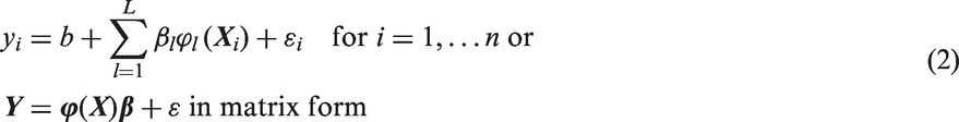
Suppose we observe a sample of $(Y, X)$ : $(Y_{i}, X_{i}), i = 1, \dots, n$ where Y_i is the observed response and $X_{i}$ a $p \times 1$ covariates vector. A SLFNN with L neurons can be represented by the following regression

y_{i} = b + \sum_{l = 1}^{L} β_{l} ϕ (b_{l} + \sum_{j = 1}^{p} w_{lj} x_{ij}) + ɛ_{i}

(1)

where b is the overall intercept, β_l are the regression coefficients, and

ɛ_{i}

independent and normally distributed error term with mean zero and constant variance σ². The

ϕ (\cdot)

function is chosen and is known as the activation function which is nonlinear and varies from (0, 1) or (−1, 1). Traditional activation functions are the logistic sigmoid or the hyperbolic tangent. Inside the activation there is a linear regression where b_l are the specific intercept and w_lj are the specific coefficients. Simply speaking, a SLFNN can be viewed as a linear combination of logistic (hyperbolic tangent) regressions.

In Figure 1 we have a graphical representation of (1) for the ith individual. We can see that in the first layer the b_l and w_lj coefficients are combined with the nonlinear function $ϕ (\cdot)$ to create the L neurons, where $ϕ_{l} (X_{i}) = ϕ (b_{l} + \sum_{j = 1}^{p} w_{lj} x_{ij})$ . Then, a linear combination of the neurons is performed to generate the output Y_i.

Figure 1.

Representation of a SLFNN.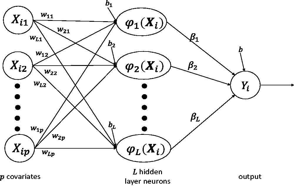

The universal approximation theorem²⁶ guarantees that under mild constraints a SLFNN with L neurons can approximate any continuous function arbitrarily well. To improve the computational cost of the SLFNNs, the ELMs randomly preassign values for all b_l and w_lj (named random feature map) and then solve a linear equation to estimate b and β_l. This prespecification step greatly speeds up the fitting of the ELM in comparison with the traditional SLFNNs. A fundamental result showed by Huang et al.³ is that even with the random feature map preselected the ELMs still have the universal approximation property and it is not sensitive to the fixed values. However, the choice of an optimum L that guarantee both good fitting and capacity of generalization (good prediction) is not a trivial task and is usually done by model selection criteria or cross validation.

For the ith observation randomly preassign values for b_l and w_lj, generated say by a N(0, 1), thus $ϕ_{l} (X_{i})$ is prespecified and known. The ELM can now be expressed as the following regression

\begin{matrix} y_{i} = b + \sum_{l = 1}^{L} β_{l} ϕ_{l} (X_{i}) + ɛ_{i} for i = 1, \dots n or \\ Y = ϕ (X) β + ɛ in matrix form \end{matrix}

(2)

Since $ϕ_{l} (X_{i})$ are known, they can be viewed as a new set of L covariates and the linear regression coefficients $β = (b, β_{1}, \dots, β_{L})^{⊤}$ can be simply estimated by minimizing the squared error by $min_{β} | | ϕ (X) β - Y | |^{2}$ .

Overfitting may be a problem in either SLFNN or ELM⁷ and regularized ELM can be used to reduce this problem. Using a l² regularization, the problem is equivalent to a ridge regression and is solved by minimizing the following objective function $min_{β} | | ϕ (X) β - Y | |^{2} + C \sum_{l = 1}^{L} β_{l}^{2}$ . An appropriate choice of the cost parameter C avoids overfit and improves the generalization characteristics of the ELM. Note that regularized ELM is a direct consequence of Bayesian modeling when a Gaussian prior is set on β_l.

3 Bayesian inference

3.1 INLA

Suppose the following hierarchical representation

\begin{array}{l} Y_{i} \sim π (y_{i} | μ_{i}, σ) \\ g (μ_{i}) = η_{i} = β_{0} + \sum_{k}^{p} β_{k} x_{i k} + \sum_{j}^{n_{f}} f^{j} (u_{j i}) + ε_{i} \end{array}

(3)

where π is a distribution density, g is an appropriate link function, β₀ is the intercept, f ^j are unknown functions of inputs U , β_k are the linear effects of input X , and

ɛ_{i}

are unstructured errors terms.

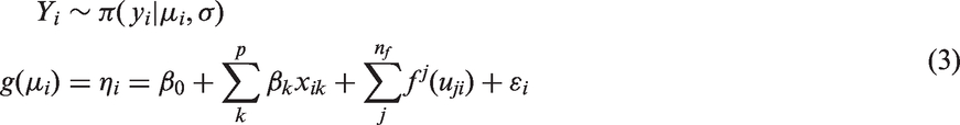
The INLA approach²⁵ performs efficient Bayesian inference over a broad class of models. The methodology relies on the latent Gaussian models structure. This is a subclass of structured additive models that can be seen as the hierarchical representation in equation (3).

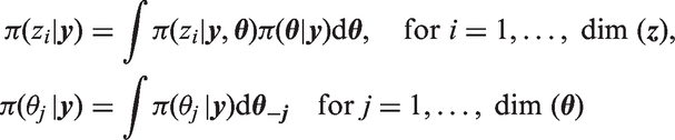
Let $z = (η^{⊤}, β^{⊤}, f^{⊤})^{⊤}$ represent the all Gaussian variables and $θ$ is the non-Gaussian variable in the model. The INLA methodology goal is to approximate the following posterior marginals

\begin{matrix} π (z_{i} | y) = \int π (z_{i} | y, θ) π (θ | y) d θ, for i = 1, \dots, dim (z), \\ π (θ_{j} | y) = \int π (θ_{j} | y) d θ_{- j} for j = 1, \dots, dim (θ) \end{matrix}

To perform the approximation of the full conditionals $π (z_{i} | y)$ and $π (θ_{j} | y)$ , INLA uses Laplace approximations combined with numerical integration routines, for more details see Rue et al.,²⁵ making the method precise and computationally efficient.

3.2 Model assessment

3.2.1 Model comparison

Recently, Gelman et al.²⁷ studied and compared a variety of model comparison criterion. Although their conclusion is that “the current state of the art of measurement of predictive model fit remains unsatisfying,” they indicate the WAIC²⁸ as one of the best current alternatives to perform model selection.

The WAIC is a fully Bayesian approach for estimating the out-of-sample expectation. The idea is to compute the log pointwise posterior predictive density (lppd) given by $lppd = \sum_{i = 1}^{n} log (\frac{1}{D} \sum_{d = 1}^{D} π (y_{i} | θ_{d}))$ , and then, to adjust for overfitting, add a term to correct for effective number of parameters $ρ_{WAIC} = \sum_{i = 1}^{n} V_{d = 1}^{D} (log π (y_{i} | θ_{d}))$ , where $V_{d = 1}^{D} (a) = \frac{1}{D - 1} \sum_{d = 1}^{D} (a_{d} - \bar{a})^{2}$ and D is the number of posterior samples generated. Finally, to set the WAIC in the deviance scale Gelman et al.²⁷ proposed that

WAIC = - 2 (lppd - ρ_{WAIC})

Thus, smaller values indicate better fit to the data.

3.2.2 Model prediction

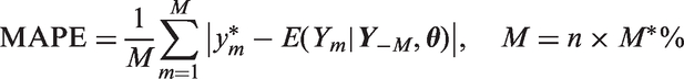
To assess the predictive power of the models we define the following steps:

A random validation sample $y_{M}^{*}$ is selected whose size is $M^{*} %$ of the total observed values. These values are not considered in the model fitting.

All proposed models are fitted with remaining values (data with validation sample removed).

Using the mean posterior parameter estimates of each fitted model, the mean of the absolute prediction error (MAPE) is computed using the validation sample $y_{D}^{*}$

MAPE = \frac{1}{M} \sum_{m = 1}^{M} | y_{m}^{*} - E (Y_{m} | Y_{- M}, θ) |, M = n \times M^{*} %

Steps 1–3 are repeated R times, where R is the number of simulations.

4 Spatial extreme learning machines (SPELMs)

Many biomedical problems are known to have spatial dependence. Inclusion of spatial random effects is common to improve fit and to better quantify uncertainty.^29–33 With the increase of data collection in recent years, missing data have become a common problem in datasets. Missing information can make traditional modeling unfeasible or very hard.

To impute data over missing values or to perform prediction, we propose a hierarchical Bayesian model that captures spatial dependence, allows for a flexible relationship between inputs and response, has generalization capability and better quantify prediction uncertainty. The model is coined as SPELMs. Let $Y = (Y_{O}, Y_{M})$ where $Y_{O}$ is the observed value with size n_O and $Y_{M}$ are missing ones with size n_M. The SPELM can be represented as

\begin{array}{l} Y_{i} \sim π (y_{i} | μ_{i}, σ) \\ g (μ_{i}) = η_{i} = b + \sum_{l = 1}^{L} β_{l} φ_{l} (X_{i}) + f^{s} (u_{i}) + ε_{i}, for i = 1, \dots, n_{O} \end{array}

(4)

where b, β_l’s, and

ϕ_{l} (\cdot)

are presented in equation (2); f ^s represents the spatial effect; and

ɛ_{i}

is an unstructured error term. This way, the SPELM introduced by equation (4) has five main advantages: (1) allow for a flexible choice of the likelihood π, e.g. Gaussian, Poisson, or Binomial; (2) combine the ELM prediction power with spatial dependence; (3) combine the computational efficiency of INLA and ELM in a Bayesian framework; (4) directly allow for l² penalization and estimation of prediction uncertainty; and (5) extension for other random effects models is straightforward, e.g. temporal and spatiotemporal models.

The predictive posterior distribution of $π (Y_{M} | Y_{O}, μ, σ)$ has all information about the n_M missing values. For example, $\hat{Y_{M}} = E (Y_{M} | Y_{O}, μ, σ)$ can be used as an estimate of the missing values. Also, credible intervals of the estimates can be directly obtained using the predictive posterior distribution.

As will be shown, the SPELMs have better point estimates of the missing value, a more parsimonious choice for the number of neurons L and better capability in controlling the prediction uncertainty when compared to the ELM.

5 Simulation study

To determine the prediction capability of ELM, SPELM, and related models, we perform a simulation study using death from lung cancer in 2010 in the municipalities of the state of Minas Gerais, Brazil. The data are freely available for download at https://mortalidade.inca.gov.br/. The Brazilian cancer control is very efficient and data are available even for small municipalities.

The World Cancer Report 2014³⁴ states that cancer is one of the most important health-related problems in developing countries. The National Cancer Institute José de Alencar da Silva is responsible by the register of cancer incidence, cancer deaths, and many other statistics related to the disease in Brazil. Lung cancer is a type of cancer that has one of the highest incidence in the world porpulation and understanding its causes is essential to perform prevention as well as control of its occurence and mortality.³⁵

Demographic information of each municipality is obtained by the 2010 Brazilian CENSUS and the following factors are used as explanatory variables: life expectancy, Gini coefficient, human development index, average income, and percent of urban areas. These variables were selected to be the same as in the real application (Section 6).

Besides having data available for all municipalities of Minas Gerais, as can be seen in Figure 2 the incidence of lung cancer somehow resembles the incidence of HIV (Section 6) where data are not fully collected. Figure 2 presents the standard incidence ratio for both lung cancer and HIV in Minas Gerais municipalities. From this figure it is also clear to verify the strong spatial association in both scenarios.

Figure 2.

Map of the standardized incidence ratio of lung cancer and HIV, respectively, in the state of Minas Gerais. (a) Lung Cancer and (b) HIV.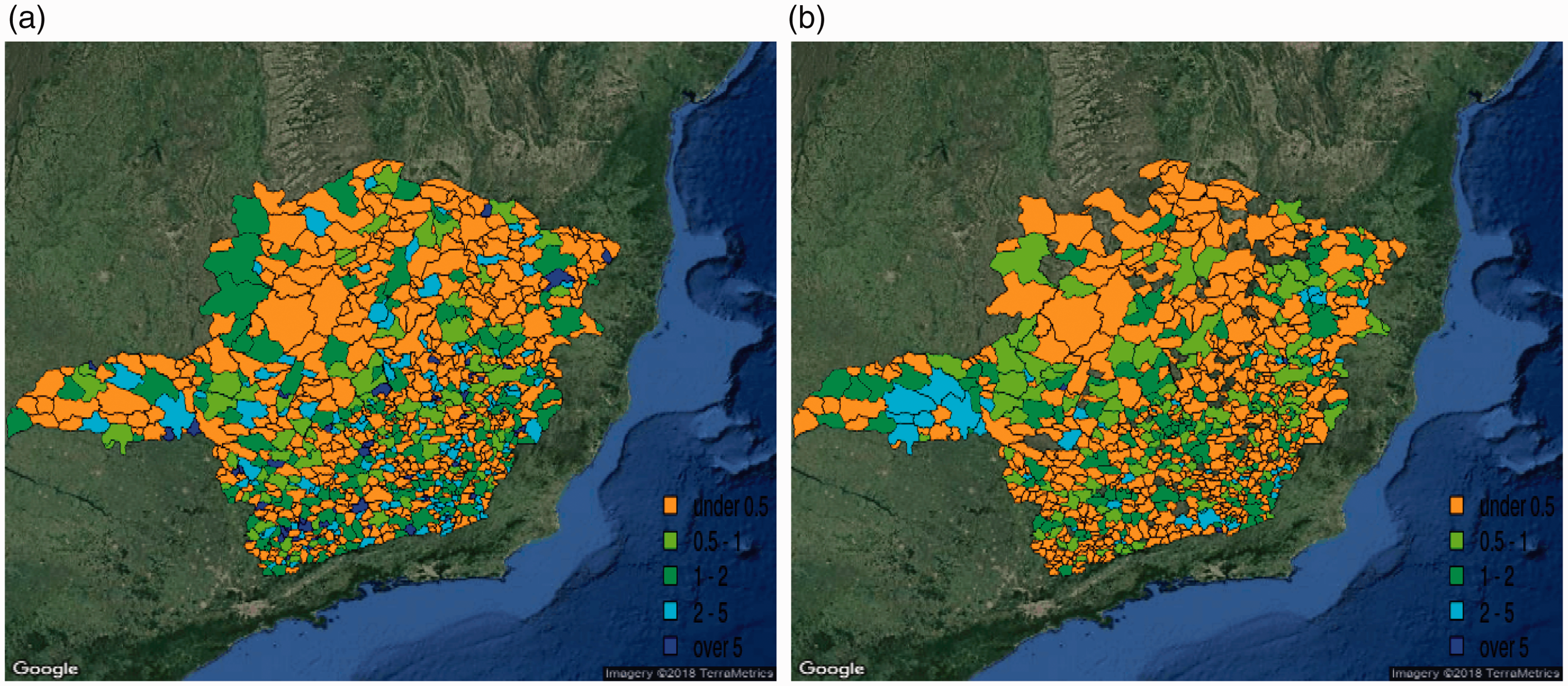

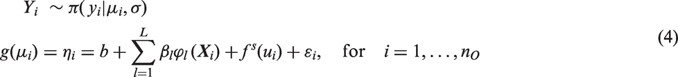
To perform prediction over missing counts we study four models as variations of equation (4) given by

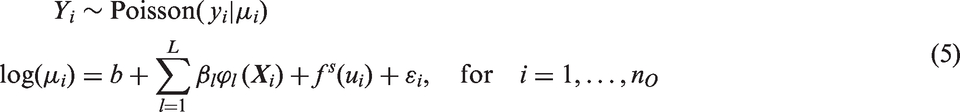
\begin{array}{l} Y_{i} \sim Poisson (y_{i} | μ_{i}) \\ \log (μ_{i}) = b + \sum_{l = 1}^{L} β_{l} φ_{l} (X_{i}) + f^{s} (u_{i}) + ε_{i}, for i = 1, \dots, n_{O} \end{array}

(5)

Model (1) is the traditional ELM (no random effects, no $f^{s} (u_{i})$ nor $ɛ_{i}$ ); Model (2) is the ELM with overdispersion ( $ɛ_{i} \sim^{iid} N (0, σ^{2})$ and no spatial effect $f^{s} (u_{i})$ —ELM-IID); Model (3) is the traditional spatial model with ICAR spatial dependence, ( $ϕ_{l} (X_{i})$ is the identity function, $f^{s} (u_{i})$ is the ICAR spatial effect, and $ɛ_{i} \sim^{iid} N (0, σ^{2})$ —SPGLM); and Model (4) is the SPELM with ICAR prior ( $f^{s} (u_{i})$ is the ICAR spatial effect and $ɛ_{i} \sim^{iid} N (0, σ^{2})$ —SPELM). For all ELM models $ϕ (\cdot)$ was chosen as the logistic activation function.

To check the models’ imputation capacity we break the simulation in two parts: (1) we use the complete data to train the model and select the number of neurons to avoid overfitting for the data improving generalization. To do so, we allow the number of neurons to vary from 2 to 30 and the cost parameter $C = (0.01, 0.02, 0.05, 1, 2, 5, 10)$ . This creates, for each proposed model, 203 configurations. To select the best fitting model we rely on the WAIC criterion that measures goodness of fit penalizing for model complexity. (2) With the selected models in hand, to check the model prediction capability, we perform a Monte Carlo study with R = 500 replicates on each scenario where we randomly set the missing information as 5, 10, and 20% of the complete data. For each replicate, to compare prediction, we calculate the MAPE for the ELM, ELM-IID, SPGLM, and SPELM.

The WAIC criterion varies with the number of neurons and cost parameter. To continue the analysis, the cost is fixed at C = 10 which provided the best results for all fitted models under the WAIC criterion for these data. Figure 3 shows the WAIC variation by the number of neurons. As it can be seen, the selected number of neurons is L = 25, L = 15, and L = 15 for the ELM, ELM-IID, and SPELM, respectively. This shows that the ELM-IID and the SPELM are more parsimonious in the number of neurons, being able to achieve the same learning with less neurons. Moreover, the SPELMs (Figure 3(c)) have a better fit for the data and the competitors’ models, since its WAIC have lower values than the other models. For the SPGLM there is no C nor L, so the model was fitted once with a WAIC_SPGLM = 2190.17 which is little higher than the WAIC_SPELM = 2186.33.

Figure 3.

(a) WAIC estimates by neurons for the ELM model, (b) WAIC estimates by neurons for the ELM-IID model, and (c) WAIC estimates by neurons for the SPELM model.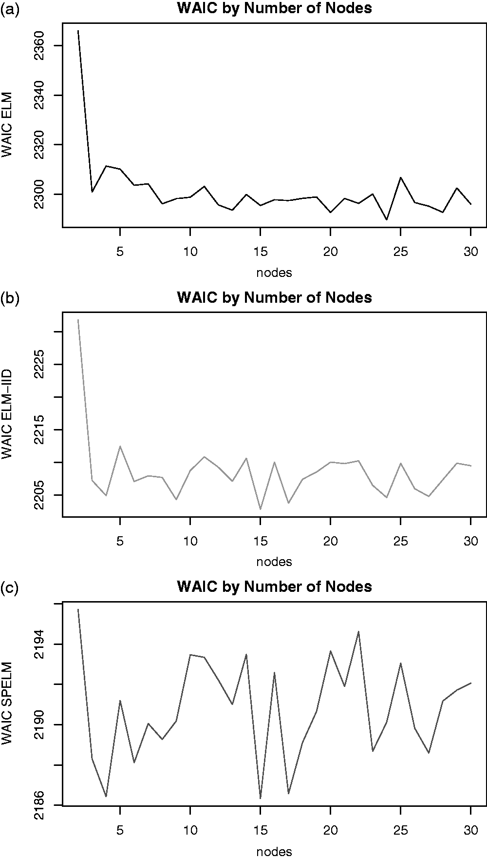

After selecting the best models fitting model in stage (1), we move to stage (2) to study the prediction potential of each model. Figure 4 shows the box plots of the MAPE for the 500 Monte Carlo replicates for the ELM, ELM-IDD, SPGLM, and SPELM. As can be seen, for all fitted models, the median of the prediction error increases as the missing percentage also increases. However, the SPELMs uniformly have better performance in the pointwise estimation than the other methods. Thus, including a spatial effect improve the prediction capacity of the ELM model. Note that the SPGLM is very competitive; however, in the SPELM, there is no restriction about the functional relationship between the mean and the covariates. This fact makes the model more robust since it can simply adapt even when this relationship is complex and far from linear.

Figure 4.

Box plot with the mean posterior prediction error of the models for the missing information of 5, 10, and 20%.

Another important characteristic to verify besides the point estimation is the coverage of the prediction interval. In other words, if the uncertainty of the prediction is adequate. From Table 1 we can see that for the 90% expected coverage probability, all fitted models are not capable to attain even near to the nominal coverage prediction probability. Although this is true for all models, the ELM-IIDs have the best performance followed very closely by the SPGLM and SPELM while the ELM method really underestimates the posterior variability of the process. The average lengths of the 90% credible interval for the ELM, ELM-IID, SPGLM, and SPELM are 0.22, 0.78, 0.75, and 0.73 which agree with the results of Table 1.

Table 1.

Coverage of the 90% predicted posterior intervals for the fitted models.

Fitted model	Coverage (in %)
Fitted model	5%	10%	20%
ELM	7	7	8
ELM-IID	31	31	31
SPGLM	29	29	29
SPELM	29	29	29

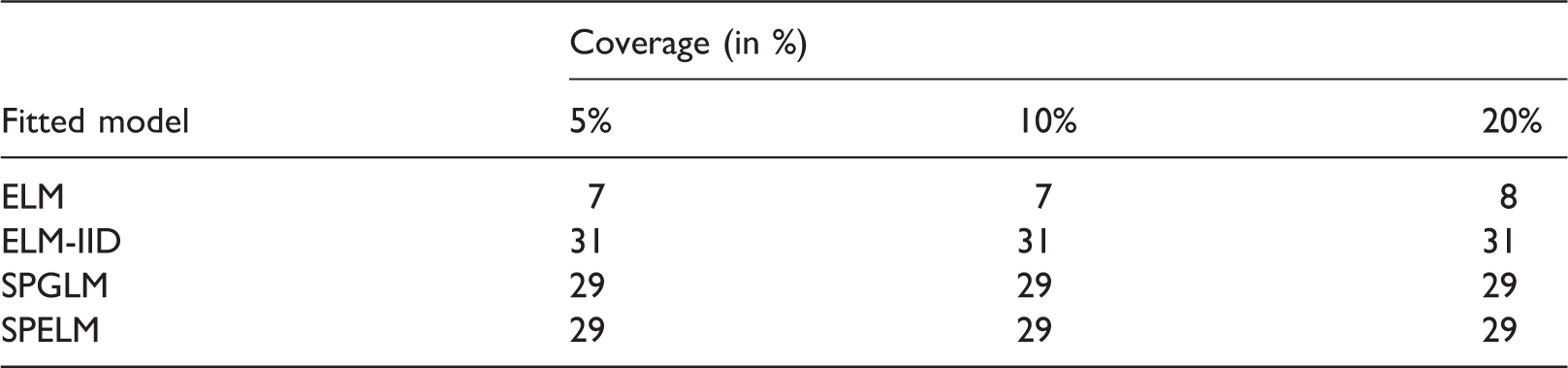
ELM: extreme learning machine; ELM-IID: extreme learning machine with overdispersion; SPELM: Spatial extreme learning machine; SPGLM: traditional generalized model with ICAR spatial effects

6 Imputing HIV data

The human immunodeficiency virus (HIV) is a chronic disease with no cure, constituting a serious public health problem. It is estimated that today 35 million people have the disease and that 54% of them are not aware that they carry the virus.³⁶ An important public health challenge is to understand the complexity and dynamics of the disease in the society, and for public policies to be effective it is necessary that more studies are conducted about the topic. Many spatial studies about HIV have been done to understand its dynamics and enlighten possible improvement in public policies (e.g. Brunello et al.,³⁷ Hixson et al.,³⁸ Thorpe et al.,³⁹ De Araujo Teixeira et al.,⁴⁰ Magalhães,⁴¹ and others).

Since 1980s, the Ministry of Health annually releases the number of new people infected with HIV for the Brazilian municipalities. Although the number of HIV infection is systematically controlled in Brazil, in practice, smaller municipalities are not able to report the number of new people infected annually, generating missing information in the available data. This missing information makes some statistical analysis harder or impracticable, especially in spatial modeling. Brazilian HIV data are freely available at http://datasus.saude.gov.br/. To make statistical analysis feasible we use the ELM, ELM-IDD, SPGLM, and SPELM to impute the missing HIV data for the state of Minas Gerais in 2010.

Magalhães⁴¹ showed that life expectancy, Gini coefficient, human development index, average income, and percent of urban areas are important covariates to explain the number of HIV new infections by municipalities in the state. These variables cover many social dimensions that are related with the HIV incidence of each municipality, e.g. life expectancy is related with the health structure; Gini coefficient, human development index, and average income are related with the wealth and job opportunity; and percent of urban areas is related with population distribution.

From the 2010 HIV report for the state of Minas Gerais, 81 out of the 853 municipalities (around 10%) of the state were unable to provide information about the number of new cases in its premises. Figure 2(b) shows the relative incidence ratio of HIV in the state. From the figure it is possible to see the missing municipalities and a clear strong spatial association in the map, which indicates that accounting for spatial dependence will improve model fitting and prediction. Following the selection model procedure presented in Section 5 we find that the best combination of the number of neurons and cost for the ELM, ELM-IID, and SPELM models are (L = 28, C = 1), (L = 4, C = 10), and (L = 4, C = 10), respectively. As we can see in Figure 5 the ELM is the only model that does not provide a good fit for the observed data. From the WAIC criterion the SPELM is the one with better fit to the data with WAIC_SPELM = 1871.97 in comparison against WAIC_ELM = 2085.51, WAIC_SPGLM = 1886.64, and WAIC_ELM_–_IID = 1873.53. As observed in Figure 5 the ELM has the worst fit which is captured by its high WAIC.

Figure 5.

Fitted values versus observed values for the ELM, ELM-IID, SPGLM, and SPELM, respectively.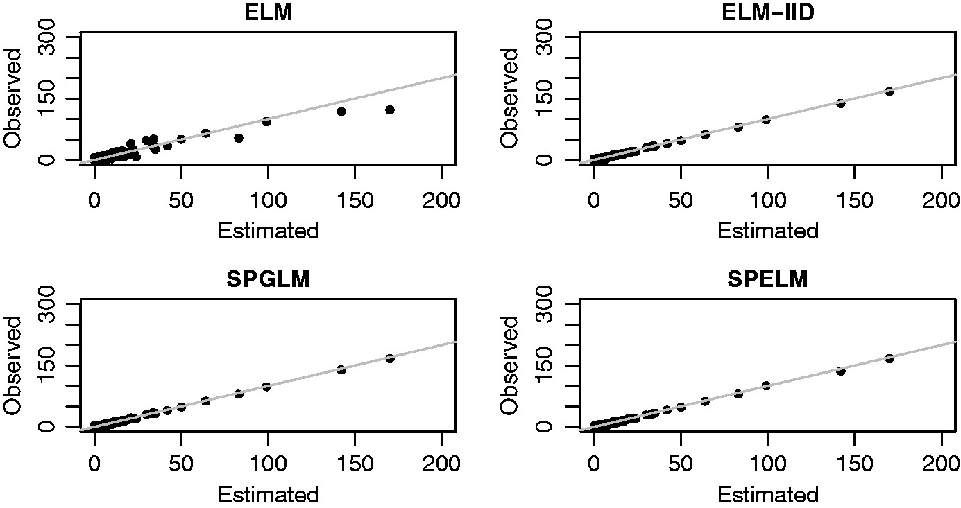

Figure 6 shows the predicted values and standard deviation of the fitted models. From the second column of figure it is clear that the ELMs have very small standard deviation which comprises its credible interval making it too narrow. Figure 6, first column, shows that the SPELM and SPGLM have predicted value that varies smoothly over the region; this is expected because both have an ICAR spatial component that capture the spatial dependence in the data while the other two models do not. Another observation is that Figure 6(a) has more extreme predicted value (low: orange areas; high: dark blue areas) than the competitors, followed by Figure 6(e) model.

Figure 6.

(a) and (b) ELM predicted value and posterior standard deviation for the missing municipalities. (c) and (d) ELM-IID predicted value and posterior standard deviation for the missing municipalities. (e) and (f) SPGLM predicted value and posterior standard deviation for the missing municipalities. (g) and (h) SPELM predicted value and posterior standard deviation for the missing municipalities. (a) ELM—prediction, (b) ELM—standard deviation, (c) ELM-IID—prediction, (d) ELM-IID—standard deviation, (e) SPGLM—prediction, (f) SPGLM—standard deviation, (g) SPELM—prediction, and (h) SPELM—standard deviation.

7 Discussion

In this paper a Bayesian SPELM is introduced. The proposed modeling strategy has many advantages: (1) it is simple yet very attractive allowing for the learning capabilities of neural networks while accommodating spatial dependence; (2) combined with INLA keeps the ELM computational efficiency even in a Bayesian framework; (3) by the intrinsic l² regularization of the method and the approximation theorem guarantee good generalization capacity; (4) easily allows for any likelihood for the response; and (5) extension for more complex models is straightforward, e.g. spatiotemporal.

From our simulation study and real data analysis we can conclude that accounting for spatial dependence make fitting and prediction more reliable and robust to spurious observations, providing more stable results when imputing the missing values. Another advantage is that the SPELM makes no restriction in the functional form of the connection between the covariates and the mean making the model more robust; this is a strong advantage in comparison with the traditional SPGLM that heavily depends on the linearity assumption. It also improves the estimation of uncertainty in prediction. However, although it has some improvement in the uncertainty estimates of the predicted values, from our simulation we can see that the improvement is still not adequate. A possible solution is to choose another likelihood for the response; this might improve model fit and help improve uncertainty estimation. This possibility will be investigated in future studies.

From the practitioners’ point of view, we think that the SPELM is a straightforward and interesting modeling alternative for the biomedical community when a nonlinear or unknown relationship between the explanatory variables and the response is observed, and, moreover, it is an adequate tool to make imputation in areal data problems with missing information.

Footnotes

Declaration of conflicting interests

The author(s) declared no potential conflicts of interest with respect to the research, authorship, and/or publication of this article.

Funding

The author(s) disclosed receipt of the following financial support for the research, authorship, and/or publication of this article: This works was partially supported by FAPEMIG and CNPq.

References

Prieto

Ortigosa

, et al. Neural networks: an overview of early research, current frameworks and new challenges. Neurocomputing 2016; 214: 242–268.

Huang

Chen

Babri

. Classification ability of single hidden layer feedforward neural networks. IEEE Trans Neural Netw 2000; 11: 799–801.

Huang

Zhu

Siew

. Extreme learning machine: theory and applications. Neurocomputing 2006; 70: 489–501.

Huang

Zhou

Ding

, et al. Extreme learning machine for regression and multiclass classification. IEEE Trans Syst Man Cybernet Part B (Cybernet) 2012; 42: 513–529.

Huang

Song

Gupta

, et al. Semi-supervised and unsupervised extreme learning machines. IEEE Trans Cybernet 2014; 44: 2405–2417.

Fernández-Delgado

Cernadas

Barro

, et al. Direct kernel perceptron (DKP): ultra-fast kernel elm-based classification with non-iterative closed-form weight calculation. Neural Netw 2014; 50: 60–71.

Lin

Liu

Fang

, et al. Is extreme learning machine feasible? A theoretical assessment (Part II). IEEE Trans Neural Netw Learn Syst 2015; 26: 21–34.

Huang

Song

, et al. Trends in extreme learning machines: a review. Neural Netw 2015; 61: 32–48.

Soria-Olivas

Gomez-Sanchis

Martin

, et al. Belm: Bayesian extreme learning machine. IEEE Trans Neural Netw 2011; 22: 505–509.

10.

Luo

Vong

Wong

. Sparse bayesian extreme learning machine for multi-classification. IEEE Trans Neural Netw Learn Syst 2014; 25: 836–843.

11.

Kim

Shin

, et al. Robust algorithm for arrhythmia classification in ecg using extreme learning machine. Biomed Eng Online 2009; 8: 31–31.

12.

Adamos

Laskaris

Kosmidis

, et al. NASS: an empirical approach to spike sorting with overlap resolution based on a hybrid noise-assisted methodology. J Neurosci Methods 2010; 190: 129–142.

13.

Savojardo

Fariselli

Casadio

. Improving the detection of transmembrane β-barrel chains with n-to-1 extreme learning machines. Bioinformatics 2011; 27: 3123–3128.

14.

Osman

Mashor

Jaafar

. Performance comparison of extreme learning machine algorithms for mycobacterium tuberculosis detection in tissue sections. J Med Imaging Health Informat 2012; 2: 307–312.

15.

Gao

Wang

Yang

, et al. A novel approach for lie detection based on f-score and extreme learning machine. PLoS One 2013; 8: e64704–e64704.

16.

MacNab

Read

Strong

, et al. Bayesian hierarchical modelling of noisy spatial rates on a modestly large and discontinuous irregular lattice. Stat Methods Med Res 2014; 23: 552–571.

17.

Piroutek

Assunção

Paiva

. Space–time prospective surveillance based on Knox local statistics. Stat Med 2014; 33: 2758–2773.

18.

Prates

Kulldorff

Assunção

. Relative risk estimates from spatial and space–time scan statistics: are they biased? Stat Med 2014; 33: 2634–2644.

19.

Riebler

Sørbye

Simpson

, et al. An intuitive Bayesian spatial model for disease mapping that accounts for scaling. Stat Methods Med Res 2016; 25: 1145–1165.

20.

Rotejanaprasert

Lawson

Bolick-Aldrich

, et al. Spatial Bayesian surveillance for small area case event data. Stat Methods Med Res 2016; 25: 1101–1117.

21.

Lawson

Banerjee

Haining

, et al. Handbook of spatial epidemiology, Boca Raton, FL: Chapman and Hall/CRC, 2016.

22.

Banerjee

Carlin

Gelfand

. Hierarchical modeling and analysis for spatial data, New York: Chapman & Hall, 2004.

23.

Besag

York

Mollie

. Bayesian image restoration with two application in spatial statistics (with discussion). Ann Inst Stat Math 1991; 43: 1–59.

24.

de Oliveira

Loschi

Assunção

. A random-censoring poisson model for underreported data. Stat Med. Epub ahead of print 2017. DOI: 10.1002/sim.7456 (accessed 24 October 2017).

25.

Rue

Martino

Chopin

. Approximate Bayesian inference for latent Gaussian models using integrated nested Laplace approximations (with discussion). J Royal Stat Soc Ser B 2009; 71: 319–392.

26.

Haykin

. Neural networks: a comprehensive foundation 2nd ed. Upper Saddle River, NJ: Prentice Hall PTR.

27.

Gelman

Hwang

Vehtari

. Understanding predictive information criteria for Bayesian models. Stat Comput 2014; 24: 997–1016.

28.

Watanabe

. Asymptotic equivalence of Bayes cross validation and widely applicable information criterion in singular learning theory. J Mach Learn Res 2010; 11: 3571–3594.

29.

Cressie

NAC

. Statistics for spatial data, USA: Wiley, 1993.

30.

Breslow

Clayton

. Approximate inference in generalized linear mixed models. J Am Stat Assoc 1993; 88: 9–25.

31.

Rue

Held

. Gaussian Markov random fields: theory and applications, Boca Raton, FL: Chapman & Hall, 2005.

32.

Leroux

Lei

Breslow

Estimation of disease rates in small areas: a new mixed model for spatial dependence. In: Halloran

Berry

(eds). Statistical models in epidemiology; the environment and clinical trials, New York: Springer-Verlag, 1999, pp. 179–192.

33.

Prates

Dey

Lachos

. A dengue fever study in the state of Rio de Janeiro with the use of generalized skew-normal/independent spatial fields. Chilean J Stat 2012; 3: 173–155.

34.

Stewart

Wild

. World cancer report 2014, Lyon: International Agency for Research on Cancer, 2014.

35.

INCA I. Estimativa 2016: incidência de câncer no Brasil. Rio de Janeiro: Ministério da Saúde, 2015.

36.

UNAIDS U. How AIDS changed everything MDG 6: 15 years, 15 lessons of hope to AIDS response. UNAIDS, 2015. Available at http://www.unaids.org/sites/default/files/media_asset/MDG6Report_en.pdf.

37.

Brunello

MEF

Neto

Arcêncio

, et al. Áreas de vulnerabilidade para co-infecção hiv-aids/tb em ribeirão preto, sp. Rev Saúde Pública 2011; 45: 556–563.

38.

Hixson

Omer

Del Rio

, et al. Spatial clustering of HIV prevalence in Atlanta, Georgia and population characteristics associated with case concentrations. J Urban Health 2011; 88: 129–141.

39.

Thorpe

Shepard

Gortakowski

, et al. Using GIS-based density maps of HIV surveillance data to identify previously unrecognized geographic foci of HIV burden in an urban epidemic. Public Health Rep 2011; 126: 741–749.

40.

de Araujo Teixeira

Gracie

Malta

, et al. Social geography of aids in brazil: identifying patterns of regional inequalities Geografia social da aids no Brasil: identificando padrões de desigualdades regionais geografía social del sida en brasil: los patrones. Cad Saúde Pública 2014; 30: 259–271.

41.

Magalhães DL. Estudo da Relação entre as Variáveis Sociais e Econômicas e o Padrão da Distribuição Espaço-Temporal dos Casos de AIDS por Município de Minas Gerais – Período entre 2000 e 2010. Master’s Thesis, Universidade Federal de Minas Gerais, Brazil, 2015.