Is the matched extreme case–control design more powerful than the nested case

Abstract

For time-to-event data, the study sample is commonly selected using the nested case–control design in which controls are selected at the event time of each case. An alternative sampling strategy is to sample all controls at the same (pre-specified) time, which can either be at the last event time or further out in time. Such controls are the long-term survivors and may therefore constitute a more ‘extreme’ comparison group and be more informative than controls from the nested case–control design. We investigate this potential information gain by comparing the power of various ‘extreme’ case–control designs with that of the nested case–control design using simulation studies. We derive an expression for the theoretical average information in a nested and extreme case–control pair for the situation of a single binary exposure. Comparisons reveal that the efficiency of the extreme case–control design increases when the controls are sampled further out in time. In an application to a study of dementia, we identified Apolipoprotein E as a risk factor using a 1:1 extreme case–control design, which provided a hazard ratio estimate with a smaller standard error than that of a 2:1 nested case–control design.

Keywords

Extreme case–control weighted likelihood matched design logistic regression power

1 Introduction

Large biobanks are valuable sources of information for genetic and molecular epidemiology. However, the amount of stored biological material is often limited and analysing it is costly. Thus, researchers are frequently forced to use case–control studies of limited size, and since the magnitude of genetic associations are often moderate, many studies have low power. This may lead to the use of non-standard sampling designs that are perceived to boost the statistical power in a specific study. One example of such a non-standard design can be found in Sboner et al.¹ In that study, men who died from prostate cancer within 10 years of diagnosis were defined as cases, and were compared to controls who were event free at least 10 years after diagnosis. The design was motivated by a conjecture that the efficiency of finding biomarkers predicting lethal prostate cancer was maximised by contrasting these two ‘extreme’ groups. The assumption was that there was underlying information in the time from diagnosis to death from prostate cancer, which seems reasonable and is intuitively appealing. However, the authors analysed the study with a logistic regression model that did not explicitly incorporate this information. In recent decades, there have also been other published studies that used a similar design, where the data also were analysed with logistic regression.^2–4

We will refer to the design used in Sboner et al.¹ as an extreme case–control (ECC) design, which we define more generally as a study that samples controls from individuals who are event-free at a pre-specified time which is either at the event time of the last case, or at a later point in time. Salim et al.⁵ suggested an alternative to logistic regression for the analysis of ECC data, proposing a method where the sampling design is taken into account in the analysis step. They considered an unconditional likelihood approach for frequency-matched controls, and a conditional approach for individually matched controls. Although the contribution of time to the sampling process is taken into account, the authors did not find any power advantage over analysis with simple logistic regression. However, their simulation studies were under-powered in many settings and they only considered a constant baseline hazard.

The nested case–control (NCC) design (incidence density sampling)⁶ is the most common sampling design for time-to-event data and is known to be close to fully efficient with four or more controls per case.⁷ The purpose of this paper is to investigate how the power of the ECC design, in particular its performance relative to the NCC design, depends on the underlying baseline hazard and the extent of the delay in sampling controls. We investigated the power of these two designs in simulation studies, and in order to understand the observed differences in power, we developed an analytical expression for the average observed information in an ECC case–control pair in a simple setting and compared it to the average observed information in an NCC pair.

2 Statistical methods

Consider a cohort of size N followed prospectively in time for an event of interest. Let τ be the end of follow-up and let t_i be the follow-up time for subject i, where t_i denotes the event-time for the cases and the censoring time for the non-cases. We assume that the event times follow the Cox proportional hazards model $h (t) = h_{0} (t) exp (β x + γ z)$ , where $h_{0} (t)$ is the baseline hazard, x the exposures of interest with associated regression coefficients $β$ , and z a vector of potential confounders with regression coefficients $γ$ .

2.1 ECC design

Assume subjects with event times smaller than τ₀ are regarded as cases and that the controls are required to be event free at time $τ \geq τ_{0}$ . When $τ = τ_{0}$ , the controls are event-free at the event-time of the last case, which is identical to the traditional case–control design. However, one could also sample more extreme controls for which $τ > τ_{0}$ . Salim et al.⁵ investigated $τ = 2 τ_{0}$ and we will also consider $τ = 3 τ_{0}$ .

Data with $τ = τ_{0}$ are routinely analysed with logistic regression, but even when $τ > τ_{0}$ , logistic regression is a valid estimator of the odds ratio. However, this approach ignores the time information. Salim et al.⁵ remarked that more careful modelling of the survival times may be advantageous and suggested both unconditional and conditional estimators. In this paper, we will focus on matched case–control studies analysed with the conditional estimator. This estimator is more robust with respect to the censoring mechanism as it only requires the censoring to be independent of covariates. In contrast, the unconditional estimator, as presented in Salim et al.,⁵ requires the censoring to be independent of t, or if it depends on t, that there is little or no censoring before τ. A derivation of the likelihood expressions for the conditional and unconditional estimators with general censoring can be found in the supplementary material. In this paper, we consider data where m controls, matched on one or more confounders, are sampled for each case. Estimation is based on fitting the following Cox regression⁵ to account for the sampling procedure for the controls

\begin{matrix} L = \underset{j \in E}{Π} \frac{exp (β x_{j}) w_{jj}}{\sum_{i \in R_{j}} exp (β x_{i}) w_{ij}} \end{matrix}

(1)

Here E is the collection of all events (cases), $R_{j}$ is the sampled risk set at event time t_j and the weight w_ij for control i in set j is given by

w_{i j} = {(\frac{S_{0} (t_{j})}{S_{0} (τ)})}^{\exp (β x_{i} + γ z_{i})}

(2)

when censoring does not depend on covariates and

S_{0} (t)

is the baseline survival at t. Intuitively, the early cases are more informative and offer a greater contrast to the controls, and this additional information is reflected in a larger weight. These weights depend on

β

and

γ

and are therefore not simple inverse sampling probabilities. Salim et al.⁵ suggested using the Kaplan–Meier method to estimate

S_{0} (\cdot)

. By noting that w_ij can be rewritten as

w_{i j} = {(\frac{S (t_{j} | x = μ_{x}, z = z_{j})}{S (τ | x = μ_{x}, z = z_{j})})}^{\exp (β (x_{i} - μ_{x}))}

(3)

then for categorical Z, we recognise

S (t_{j} | x = μ_{x}, z = z_{j})

as the survival function for a subject in stratum

z_{j}

with average exposure, denoted by

μ_{x}

. Assuming that the event is rare, we can approximate

S (t_{j} | x = μ_{x}, z = z_{j})

and

S (τ | x = μ_{x}, z = z_{j})

using the KM estimates based on the full cohort, where separate curves are estimated for different strata defined by Z. The estimate of w_ij is then given by replacing

S (\cdot)

with its estimate

\hat{S} (\cdot)

and

μ_{x}

with

\bar{x}

in equation (3).

The regression coefficient $β$ is obtained by maximizing the likelihood L in equation (1) and the variance estimate of $β$ is obtained from the inverse of the information matrix which is available numerically from the optimization routine. The interpretation of $β$ is a log-hazard ratio. The full derivation of the likelihood expression can be found in the supplementary material.

As noted above, both weighted Cox regression and logistic regression are valid methods of analysis for ECC data. However, the two regression models have different target parameters, the hazard ratio and odds ratio, respectively. In addition, the weighted Cox regression is only valid for rare events, while logistic regression is always a valid estimator of the odds ratio.

2.2 NCC design

In a NCC design, the m controls sampled for each case are required to be event-free at the event-time of the case, and may also be matched on additional factors. The traditional way of analysing NCC data is by stratified Cox regression, or equivalently conditional logistic regression, each of which maximises the following (partial) likelihood when all confounders have been matched

\begin{matrix} L' = \underset{j \in E}{Π} \frac{exp (β x_{j})}{\sum_{i \in R_{j}} exp (β x_{i})} \end{matrix}

(4)

The regression coefficients are interpreted as log-hazard ratios and the partial likelihood has the usual likelihood properties.⁸

3 Simulation study

Sboner et al.¹ wrote that the efficiency of finding signature genes predicting prostate cancer was maximised by comparing cases with the ‘extreme’ controls which were required to be event-free 10 years after diagnosis. Those controls were ‘long-term survivors’ and the underlying assumption was that there was information in the follow-up time. The expression for w_ij above facilitates an investigation of how this information is reflected in the power of the ECC designs with different baseline hazards and different τ (minimum survival time of a control), for a given τ₀ (time of last event).

We simulated cohorts of size 50,000 where the underlying baseline hazard was either constant $h_{0} (t) = λ$ = 0.0111, or linearly increasing $h_{0} (t) = \tilde{λ} t = 0.001 t$ . For the constant baseline hazard, the event times were drawn from a Weibull distribution with rate $λ exp (β x + γ z)$ and shape = 1, while for the increasing baseline, the rate was $\tilde{λ} exp (β x + γ z)$ , and shape = 2. We also simulated a censoring time for each subject which was exponentially distributed with rate = 0.05 and the follow-up time of each subject was the minimum of the event time and the censoring time. To evaluate the sensitivity to the independent censoring assumption, we also simulated censoring times with rate = 0.04 for unexposed and either 0.06 or 0.2 for exposed. This induced a correlation between the exposure and censoring of approximately −0.1 and −0.3.

The covariates x and z were simulated as binary variables: the confounder z was Bernoulli with parameter = 0.5, and we introduced a relationship between exposure x and the confounder z by a logistic regression model for the probability of being exposed, $exp (- 2 + g z) / (1 + exp (- 2 + g z))$ with g taking values 0.5 or 1. We chose values for β of $log (1.2) = 0.182$ and $log (1.5) = 0.405$ to be representative of genetic studies where the effect sizes are usually moderate.

In the ‘extreme design’, subjects with $t < τ_{0}$ and with an uncensored event time were considered to be cases and τ₀ was chosen large enough for the ECC study with $τ = τ_{0}$ and one control per case to have approximately 50% power. To achieve this, τ₀ was set at the time required to observe 1700 and 320 events (3.4% and 0.6% of the total cohort size) for hazard ratios of 1.2 and 1.5, respectively.

For each case, we sampled controls corresponding to $τ = τ_{0}, τ = 2 τ_{0}$ and $τ = 3 τ_{0}$ and for each setup we sampled one, two and three controls per case matched on z. Since the ‘extreme’ designs are to be compared to the NCC design with regard to power, we also sampled one, two and three controls matched on z at the event times, i.e. risk set sampling.

The ECC data were analysed with the weighted method, equation (1) and logistic regression. The NCC data were analysed with a stratified Cox regression, equation (4). The simulations were conducted 500 times and the power was estimated as the proportion of times the 95% confidence interval for the hazard ratio did not include one. All simulations were carried out using R version 3.3.2.⁹

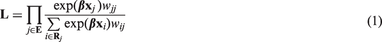
Figure 1 displays the power for the analyses with the weakest confounding by z (g = 0.5) and one control per case. The power increases over time for the extreme designs, except for $β = log (1.5)$ and constant baseline in which case the power is approximately constant. The extreme designs have similar power in all scenarios for both estimation methods and higher than the power of NCC. For increasing baseline, there is a substantial power gain already at $τ = τ_{0}$ for the ‘extreme’ designs compared to the NCC design, and the power continues to increase at $2 τ_{0}$ and $3 τ_{0}$ , particularly for $β = log (1.2)$ . When comparing the power at $2 τ_{0}$ for constant and increasing baseline for $β = log (1.2)$ , it is clear that the power is higher for increasing baseline, and even more pronounced at $3 τ_{0}$ .

Figure 1.

Power of ECC at τ₀, 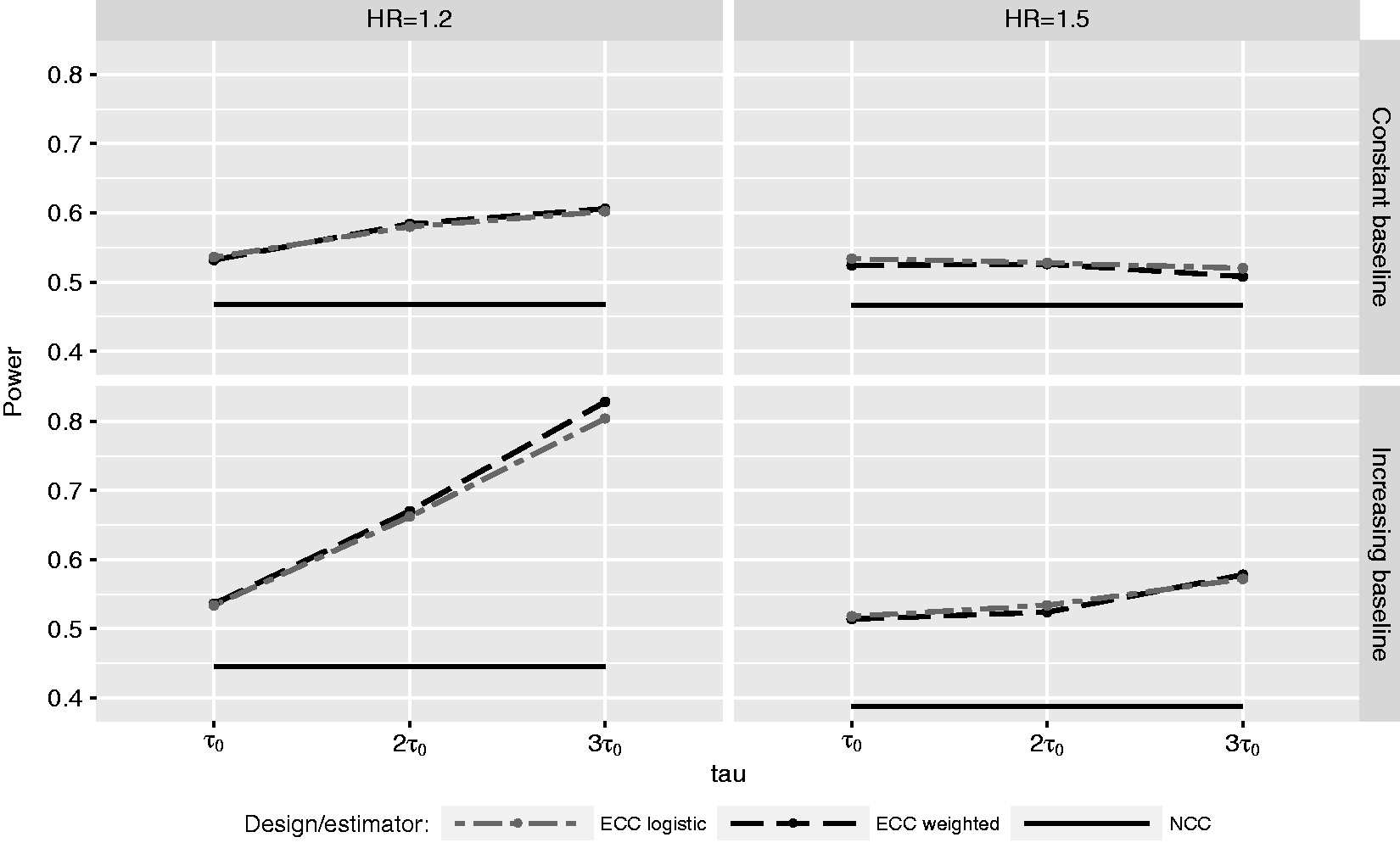$2 τ_{0}$ and $3 τ_{0}$ . ECC data analysed with proposed weighted method and logistic regression, and NCC design analysed with conditional logistic regression. Studies have 1700(HR = 1.2) and 320(HR = 1.5) cases with each cases matched to one control on a weak confounder z.

With the strongest confounding by z (g = 1), the overall picture is similar (Figure 2) but the power advantage of the ‘extreme’ design is somewhat higher at 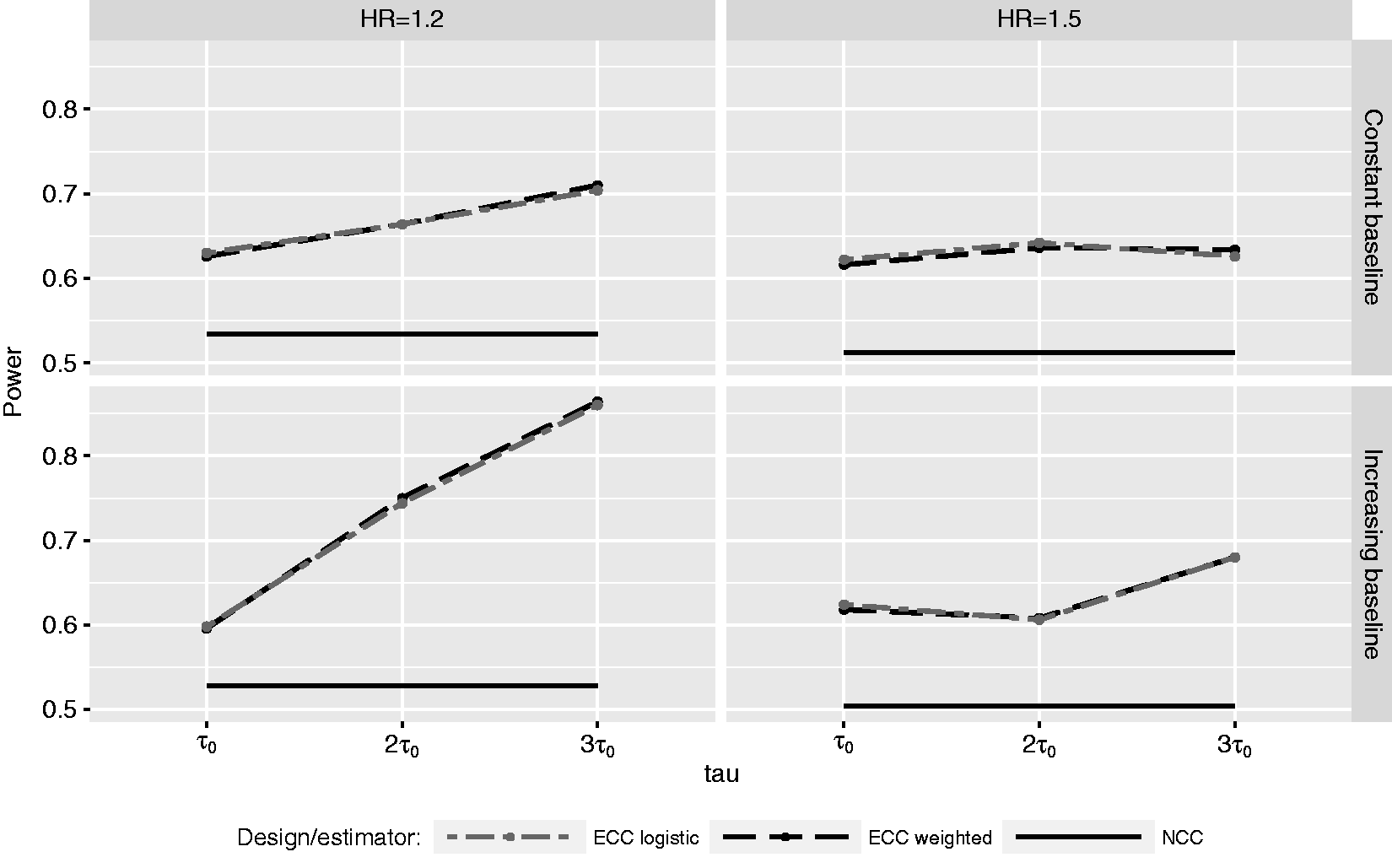$τ = τ_{0}$ for the constant baseline than in Figure 1. The results for 2 and 3 controls per case follow Figures 1 and 2 closely and can be found in the supplementary material.

Figure 2.

Table 1 presents the bias, standard error and type I error or power from all designs with one control per case, constant baseline hazard and the weakest confounding. All estimates are unbiased except those from the unadjusted cohort analyses where there is considerable bias, as expected. The empirical and estimated standard errors are in good agreement and the type I errors are close to 0.05. The corresponding table for increasing baseline hazard is reported in the Supplementary Material, Table S1. For the strongest confounding by z, the results are similar, but with a larger bias in the estimates from the unadjusted cohort analysis (results not shown). Tables S2 and S3 in the Supplementary Materials show the simulation results when censoring is weakly and moderately dependent on exposure. The empirical and estimated standard errors are in good agreement, but the estimates from ECC are biased. The bias is increasing for increasing τ and larger when there is stronger dependence between exposure and censoring time.

Table 1.

Simulation results for one control per case, constant baseline hazard and weakest confounding by z.

	Bias (β)	Est. se	Emp. se	Type I error/power
Design	$β = log (1) = 0$
Cohort unadj.	0.095	0.151	0.153	0.110
Cohort adj.	−0.016	0.152	0.153	0.038
ECC $τ = τ_{0}$	−0.015	0.215	0.216	0.054
ECC $τ = 2 τ_{0}$	0.003	0.217	0.217	0.044
ECC $τ = 3 τ_{0}$	−0.002	0.219	0.211	0.046
NCC	0.001	0.227	0.227	0.044
	$β = log (1.2) = 0.182$
Cohort unadj.	0.130	0.062	0.062	0.998
Cohort adj.	0.001	0.062	0.062	0.834
ECC $τ = τ_{0}$	−0.001	0.088	0.083	0.532
ECC $τ = 2 τ_{0}$	−0.002	0.084	0.088	0.584
ECC $τ = 3 τ_{0}$	−0.002	0.080	0.082	0.606
NCC	−0.001	0.097	0.097	0.468
	$β = log (1.5) = 0.405$
Cohort unadj.	0.104	0.134	0.137	0.942
Cohort adj.	−0.013	0.134	0.138	0.810
ECC $τ = τ_{0}$	−0.001	0.204	0.193	0.524
ECC $τ = 2 τ_{0}$	−0.004	0.202	0.202	0.526
ECC $τ = 3 τ_{0}$	−0.012	0.199	0.198	0.508
NCC	−0.001	0.222	0.234	0.466

Bias: mean of estimates – true value; Est. se: mean of estimated standard error; Emp. se: standard deviation of estimates; Type I error/power: proportion of estimates within 95% confidence interval; Cohort unadj./adj.: Cox regression of full cohort not adjusted/adjusted for z; ECC: extreme case–control data; NCC: nested case–control data.

4 Variance comparison

To understand the contributions to the higher power of the ECC design, we compared the variance estimators from the two designs by using the information matrix. For simplicity, we consider a binary exposure and a $1 : 1$ case–control ratio. We plot a quantity which we refer to as the average information which we motivate as follows: due to the conditional nature of the likelihood, each information contribution is from a case–control pair and not from a single individual. The information is defined as $I_{j} = - \frac{\partial^{2}}{\partial β^{2}} log (L_{j})$ where $\frac{\partial^{2}}{\partial β^{2}} log (L_{j})$ is the second-order derivative of the log-likelihood with respect to β. It is clear that, similar to the NCC design, concordant pairs do not contribute to the information. Additionally, it is not informative to examine the ‘crude’ information over time from a particular case–control pair with specific covariates since the probability of such a pair occurring will change over time depending on the hazard ratio and the prevalence of exposure. A more reasonable quantity to consider is the following, which we will refer to as the average information in a pair

J_{j} = J (t_{j}, τ) = I_{j}^{1} p^{1} + I_{j}^{0} p^{0}

(5)

where superscript 1 refers to a pair with an exposed case (and thus unexposed control), superscript 0 refers to a pair where the case is unexposed (and control exposed), and p₁ and p₀ are the probabilities of sampling such pairs. Thus, our average information is the sum of the two types of informative pairs multiplied by the probabilities of obtaining such pairs if the case occurs at time t_j and the control survives event-free until at least time τ (see Appendix 1 for details).

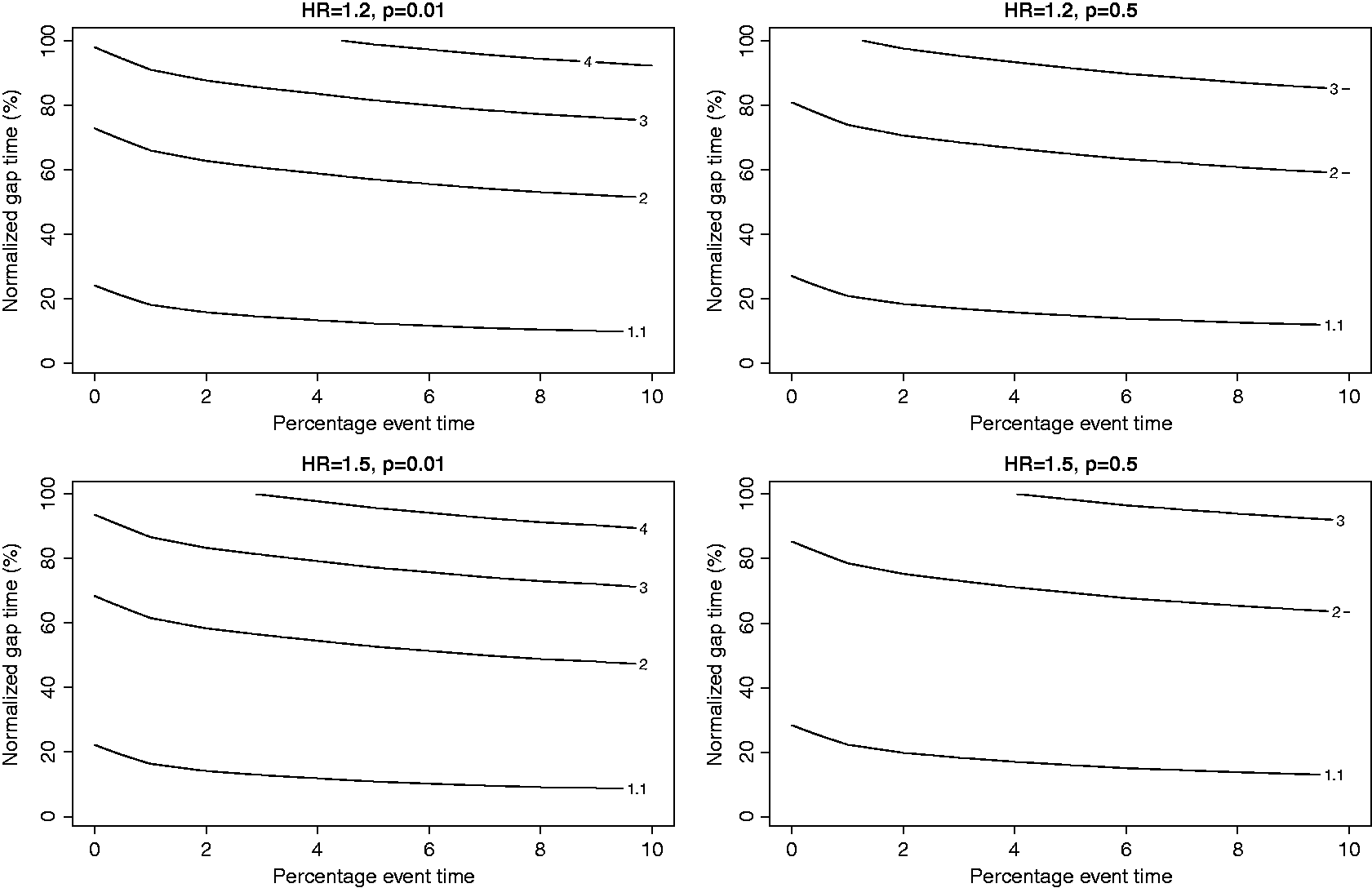
As before, we consider constant and linearly increasing baseline hazards and hazard ratios of {1.2, 1.5}. The baseline exposure prevalence is set at 0.01 and 0.5. In each scenario, we let the event times range from 0+ to τ₀ which we fix at a specified decile, α₀ of the given survival distribution (assuming no censoring). We chose the first decile, hence $τ_{0} (α_{0}) = τ_{0} (0.1)$ and the controls are sampled from $τ_{0} (0.1)$ up to the third quartile of the survival distribution, $τ (α) = τ (0.75)$ , see Figure 3. We also define the ‘gap time’ as the difference between the sampling time of a control and the event time of the corresponding case. The average information in the NCC design is calculated at each event time with $τ = t_{j}$ .

Figure 3.

Schematic representation of one case–control configuration. Probability distribution function of event times. T_e and T_c are a particular event and sampling time, respectively. Cases occur before 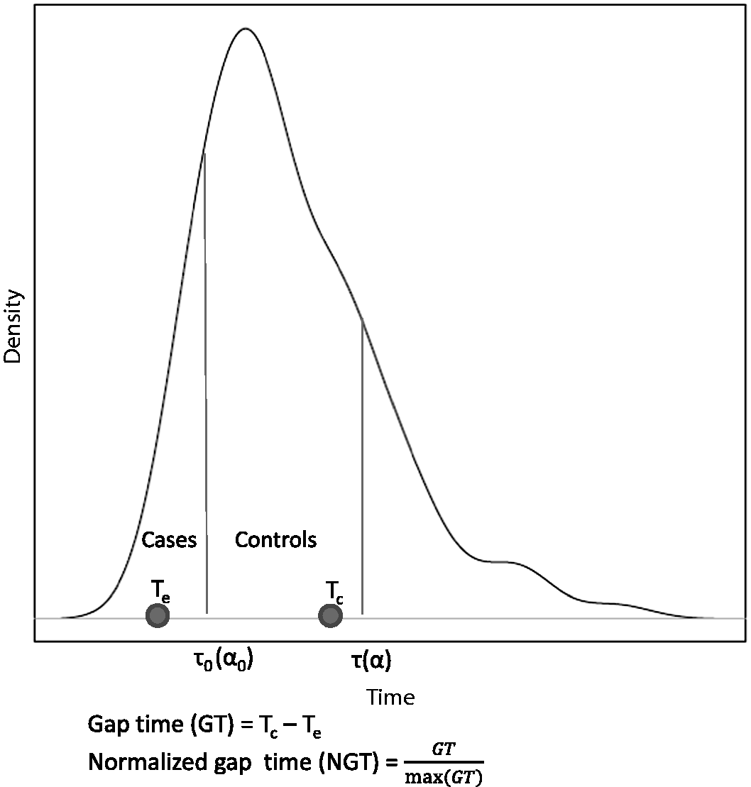$τ_{0} (α_{0})$ and controls are sampled from $τ_{0} (α_{0})$ up to $τ (α)$ with α₀ and α being percentiles in the distribution of the event times. max(GT) is the time between first case and last possible control.

The contour plots of average information in an ECC pair relative to the average information in a NCC pair for four combinations of hazard ratio and baseline exposure prevalence are given in Figure 4 for constant baseline and in Figure 5 for increasing baseline. The x-axis denotes the percentile of the survival distribution (from zero to $τ_{0} (0.1)$ ) and the y-axis denotes the gap time which has been normalized so that 100 represents the time between the first case and the last possible control. The values of the contour lines denote the relative average information in an ECC design compared to the NCC design. The relative information will only equal one when the gap time is zero, i.e. when the control is sampled at the event time of the case. Since this only occurs at the last event time in the ECC design, the smallest contour lines are drawn at a relative information of 1.1.

Figure 4.

Contour plots of relative average information for a constant baseline for combination of hazard ratios and exposure prevalence. X-axis: event times, ranging from 0+ to the first decile. Y-axis: normalised gap time between event time and sampling time in percent with 0 representing control sampled at the event time of the case and 100 the gap time between the first case and the last control sampled at the third quartile of the survival distribution.

Figure 5.

Contour plots of relative average information for an increasing baseline for combination of hazard ratios and exposure prevalence. X-axis: event times, ranging from 0+ to the first decile. Y-axis: normalised gap time between event time and sampling time in percent with 0 representing control sampled at the event time of the case and 100 the gap time between the first case and the last control sampled at the third quartile of the survival distribution.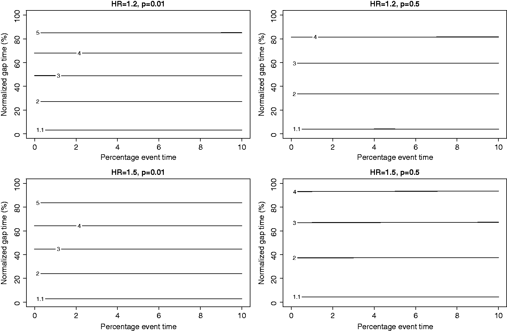

From Figure 4, we see that with a constant baseline hazard, the average information is always higher for the ECC design than for the NCC design. The horizontal contour lines indicate that it is only the time difference between the case and the control that governs the information increase of the ECC design. It is also seen that to obtain the same relative increase in information, a shorter gap time is required for the rare exposure compared to the common exposure. For a rare exposure, the ECC design is relatively more informative for larger hazard ratios, while for a balanced exposure, the relative information is larger for smaller hazard ratios.

For the increasing hazard ratio (Figure 5), the contour lines are no longer horizontal but have a negative gradient, indicating that the event times also influence the relative information and for larger event times a smaller gap time is required to obtain the same amount of relative information compared to the earlier cases. This seems reasonable since the cases will occur more and more frequently and a specific gap time early in the process is somehow less ‘extreme’ than the same gap time later in the process. Apart from this, the plots display the same features as Figure 4 with respect to exposure prevalence and gap times.

5 Data analysis

As an illustration, we analysed the association between the Apolipoprotein E (APOE) $ɛ 4$ allele and dementia. APOE is a polymorphic gene with three major alleles $ɛ 2, ɛ 3$ and $ɛ 4$ , and $ɛ 4$ has been shown to be associated with dementia¹⁰ and particularly with Alzheimer’s disease.¹¹ Our data consist of a small cohort of opposite-sex twins called GENDER¹² recruited from 1995 to 1997 with a mean age of 75 and followed up for diagnosis of dementia or death until the end of 2012. After excluding prevalent cases (n = 19), our data set consisted of 466 subjects including 126 cases of dementia. The use of these data was approved by the Ethics Review Committee at Karolinska Institutet (ethical approval number 03:124 and 2007-151-31-4).

From Figure 6, we see that the baseline hazard is increasing from approximately year 10 of the follow-up in our data set. For the ECC sampling design, we define a dementia case to be a subject experiencing dementia within 10 years of inclusion in the study (76 cases) and we sample controls from the 153 individuals who are alive and dementia-free 15 years after inclusion, i.e. 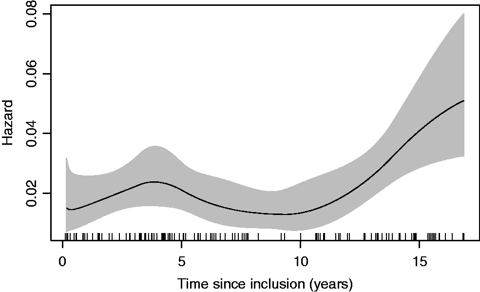$τ = 1.5 τ_{0}$ . The controls are not matched in the traditional sense, but we require that they are not the case’s co-twin and we therefore use the conditional estimator for the ECC design. For the NCC design, we use the same 76 cases but the time-matched non-twin controls are only required to be alive and event-free at the event time of the case. The NCC data are analysed with the traditional conditional logistic regression estimator (stratified Cox regression). For comparison, we do a full cohort analysis where we fit a shared frailty model with a gamma distributed frailty to take care of the twin dependencies in the data, using the R-package frailtypack.^13,14

Figure 6.

Baseline hazard of dementia from full data estimated with a flexible parametric model¹⁵ using the rstpm2-package¹⁶ in R with 5 knots.

The results presented in Table 2 indicate that the presence of the

ɛ 4

allele approximately doubles the risk of developing dementia. Adjustment for cardiovascular disease or for educational level (shorter or longer than seven years) did not change the results (data not shown). Although the estimate from the 1:1 ECC analysis is somewhat smaller than the cohort estimate, it is not biased in the sense that the confidence interval covers the cohort estimate. The ECC design is also clearly more efficient than the NCC design and is close to fully efficient with two controls per case.

Table 2.

Results from the dementia data.

Design	n/case	HR (95% CI)	Se(β)
Cohort	466/126	1.96 (1.31–2.93)	0.206
ECC 1:1	152/76	1.68 (1.05–2.69)	0.240
NCC 1:1	152/76	2.08 (1.07–4.03)	0.338
ECC 2:1	228/76	2.28 (1.53–3.40)	0.204
NCC 2:1	228/76	1.81 (1.01–3.26)	0.300

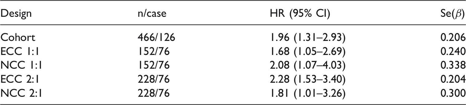
ECC: extreme case–control; NCC: nested case–control.

6 Discussion

We have investigated the power of the ECC design and compared it to the NCC design. Our main conclusions are that an ECC design may be more powerful than the NCC design, with the gain increasing with increasing time gap between the sampling of cases and controls. In the dementia analysis, the standard error of the hazard ratio in the 1:1 ECC design was smaller than the corresponding standard error for the 2:1 NCC design. Secondly, our investigations confirmed the findings of Salim et al.⁵ that there is almost no gain in power using the estimators they suggest compared to a simple logistic regression. However, an important advantage of using the weighted Cox regression is that we can estimate hazard ratios instead of odds ratios. The size of the hazard ratio does not depend on the follow-up time τ₀, and it therefore provides a parameter estimate that is comparable with other studies and will lend itself to future meta analyses. The drawback is, of course, that the estimation is somewhat more complicated since the likelihood must be optimized numerically.

In this paper, we show that there can be substantial power gains when the controls are sampled after τ₀. This contrasts with previously reported minor differences,⁵ which may have been due to a lack of power especially for the smallest β (where we found the largest power gain). In addition, we found the largest gain for an increasing baseline hazard which has not been investigated previously.

The contour plots in Figures 4 and 5 showed that for the same percentage event time and normalized gap time, the relative information gain from ECC is larger under constant hazards. This may seem surprising at first, especially since our simulation studies demonstrated greater power gain under an increasing baseline hazard. These seemingly contrasting results can be explained by the fact that in the simulation studies, the threshold for early cases (τ₀) under a constant baseline hazard was much earlier than the threshold for early cases under the increasing baseline hazard (Supplementary Figure 5). Since we choose the gap time in the simulation studies as multiples of τ₀, this results in wider gap times for simulations where τ₀ is larger, in this case under the increasing hazards. Hence, the power gain we observe in the simulation studies under the increasing baseline hazard is primarily due to larger gap times, which is consistent with our observations from the relative information plots.

In practice, sampling controls at specific percentiles of the survival distribution may be difficult due to censoring. We therefore chose to use the one, two and three times τ₀ ‘rule’ for sampling controls in the simulations and we refer to such controls as ‘extreme’. It is, however, important to think about where/when τ₀ and τ are defined, because depending on where we fix τ₀ in the survival process, a time point that is a factor of two and three times larger might or might not be an ‘extreme’ survival time. Additionally, it is important to keep in mind the duality of $τ_{0} = τ_{0} (α_{0})$ and $τ = τ (α)$ . From Figure 3, it is clear that with 1 control per case α cannot be larger than $1 - α_{0}$ . This means that the more cases that are included, the less extreme the controls can be, in order to ensure sufficient subjects at risk at τ.

Some caution is required regarding the weighted estimator. Firstly, the weights given in equation (2) are only valid when censoring does not depend on covariates, so further work is needed to derive weights that could account for this type of dependent censoring. Secondly, we assume time-constant coefficients, so if this assumption does not hold, there is no clear interpretation of the estimate of β, in contrast to a cohort analysis where it is the weighted average of the time-varying coefficients.¹⁷

We have motivated the use of ECC for situations where limited and expensive material (e.g. from a biobank) is to be used so that selecting the most informative cases and controls can be important in order to make efficient use of valuable resources.¹⁸ However, in studies of rare diseases, the main limitation is slow accrual of cases, so that (i) sampling only the earliest cases may be too costly in terms of power, and (ii) by the time sufficient cases have been identified, extending the follow-up to obtain more extreme controls too costly in terms of time. In such situations, an NCC design may be the best choice.

In summary, we have shown that ‘extreme’ case–control designs may be more powerful than the NCC design. We have also shown that with regard to power, a simple logistic regression analysis is no less powerful than the somewhat more complicated weighted Cox regression. Thus, the purpose of the study becomes important when choosing the method of analysis: if the only motivation is discovery, for example identification of significant molecular or genetic markers, the logistic model is adequate. However, if the effect sizes are of interest, the weighted Cox regression is a better choice since the estimated hazard ratios enable comparison with other work and a contribution to meta-analyses.

Supplemental Material

Supplemental material for Is the matched extreme case–control design more powerful than the nested case–control design?

Supplemental Material for Is the matched extreme case–control design more powerful than the nested case–control design? by NC Støer, A Salim, K Bokenberger, I Karlsson and M Reilly in Statistical Methods in Medical Research

Footnotes

Declaration of conflicting interests

The author(s) declared no potential conflicts of interest with respect to the research, authorship, and/or publication of this article.

Funding

The author(s) disclosed receipt of the following financial support for the research, authorship, and/or publication of this article: This work was supported in part by the Swedish Cancer Society [Grant number CAN 2009/1175 and CAN 2015/493].

Supplemental material

Supplemental material for this article is available online.

Appendix 1

References

Sboner

Demichelis

Calza

, et al. Molecular sampling of prostate cancer: a dilemma for predicting disease progression. BMC Med Genom 2010; 3: 1–12.

Miller

Førde

Thelle

, et al. The Tromsø heart-study – high-density lipoprotein and coronary heart disease: a prospective case–control study. Lancet 1977; 1: 965–968.

Després

Lamarche

Mauriège

, et al. Hyperinsulinemia as an independent risk factor for ischemic hart disease. N Engl J Med 1996; 334: 952–958.

Danesh

Wheeler

Hirschfield

, et al. C-reactive protein and other circulating markers of inflammation in the prediction of coronary heart disease. N Engl J Med 2004; 350: 1387–1397.

Salim

Fall

, et al. Analysis of incidence and prognosis from ‘extreme’ case–control designs. Stat Med 2014; 33: 5388–5398.

Thomas

. Addendum to: “methods of cohort analysis: appraisal by application to asbestos mining” by Liddell FDK, McDonald JC and Thomas DC. J R Stat Soc 1977; 140: 469–491.

Goldstein

Langholz

. Asymptotic theory for nested case–control sampling in Cox regression models. Ann Stat 1992; 20: 1903–1928.

Borgan

Samuelsen

Nested case–control and case–cohort studies. In: Klein

Houwlingen

Ibrahim

, et al.(eds). Handbook of survival analysis, London: Chapman and Hall, 2013, pp. 346–347.

R Core Team. R: a language and environment for statistical computing, Vienna, Austria: R Foundation for Statistical Computing, 2014.

10.

Hofman

Ott

Breteler

MMB

, et al. Atherosclerosis, apolipoprotein E, and the prevalence of dementia and Alzheimer’s disease in the Rotterdam Study. Lancet 1997; 349: 151–154.

11.

Farrer

Cupples

Haines

, et al. Effects of age, sex and ethnicity on the association between Apolipoprotein E genotype and Alzheimer disease. J Am Med Assoc 1997; 278: 1349–1356.

12.

Gold

Malmberg

McClearn

, et al. Gender and health: a study of older unlike sex-twins. J Gerontol 2002; 57B: 168–176.

13.

Rondeau

Gonzalez

. Frailtypack: a computer program for the analysis of correlated failure time data using penalized likelihood estimation. Comput Meth Prog Biomed 2005; 80: 154–164.

14.

Rondeau

Mazroui

Gonzalez

. frailtypack: an R package for the analysis of correlated survival data with frailty models using penalized likelihood estimation or parametrical estimation. J Stat Software 2012; 47: 1–28.

15.

Royston

Parmar

MKB

. Flexible parametric proportional-hazards and proportional-odds models for censored survival data, with application to prognostic modelling and estimation of treatment effects. Stat Med 2002; 21: 2175–2197.

16.

Clements M and Liu XR. rstpm2: flexible link-based survival models, http://CRAN.R-project.org/package=rstpm2 [R package version 1.2.2] (2015, accessed 10 May 2018).

17.

Struthers

Kalbleisch

. Misspecified proportional hazard models. Biometrika 1986; 73: 363–369.

18.

Lash

Schisterman

. New designs for new epidemiology. Epidemiology 2018; 29: 76–77.

19.

Aalen

Borgan

Gjessing

. Survival and event history analysis (statistics for biology and health), 1st ed. New York: Springer, 2008, pp. 196–197.

Supplementary Material

Please find the following supplemental material available below.

For Open Access articles published under a Creative Commons License, all supplemental material carries the same license as the article it is associated with.

For non-Open Access articles published, all supplemental material carries a non-exclusive license, and permission requests for re-use of supplemental material or any part of supplemental material shall be sent directly to the copyright owner as specified in the copyright notice associated with the article.

0.00 MB

0.22 MB