
Abstract
This paper concerns estimation of subgroup treatment effects with observational data. Existing propensity score methods are mostly developed for estimating overall treatment effect. Although the true propensity scores balance covariates in any subpopulations, the estimated propensity scores may result in severe imbalance in subgroup samples. Indeed, subgroup analysis amplifies a bias-variance tradeoff, whereby increasing complexity of the propensity score model may help to achieve covariate balance within subgroups, but it also increases variance. We propose a new method, the subgroup balancing propensity score, to ensure good subgroup balance as well as to control the variance inflation. For each subgroup, the subgroup balancing propensity score chooses to use either the overall sample or the subgroup (sub)sample to estimate the propensity scores for the units within that subgroup, in order to optimize a criterion accounting for a set of covariate-balancing moment conditions for both the overall sample and the subgroup samples. We develop two versions of subgroup balancing propensity score corresponding to matching and weighting, respectively. We devise a stochastic search algorithm to estimate the subgroup balancing propensity score when the number of subgroups is large. We demonstrate through simulations that the subgroup balancing propensity score improves the performance of propensity score methods in estimating subgroup treatment effects. We apply the subgroup balancing propensity score method to the Italy Survey of Household Income and Wealth (SHIW) to estimate the causal effects of having debit card on household consumption for different income groups.
Keywords
1 Introduction
A central goal in comparative effectiveness research is to estimate the causal effect of a treatment unconfounded by differences between characteristics of subjects assigned to alternative treatment conditions. Comparisons between groups can be biased when the groups are unbalanced with respect to confounders. Propensity score methods 1 have been widely used as a robust approach to achieve covariate balance and draw causal inferences in observational studies.2,3 The propensity score is the probability that a unit is assigned to one treatment condition; balance of the propensity score leads to balance of the multivariate covariates.
Causal inference has traditionally focused on average treatment effects for the overall population. However, heterogeneity in treatment effects across different subpopulations is the norm rather than exception in medical research. Patients with the same medical condition but different age, gender, race and risk profile usually respond to the same treatment differently.
4
Research on heterogeneous treatment effects (HTE) has received increasing attention in recent years, where the goal is to identify the subpopulations who are the most or the least responsive to a treatment. In this paper, we focus on a specific type of HTE analysis, namely the propensity-scores-based subgroup analysis (SGA), which aims at estimating the causal effects of the subgroups that are pre-defined by one or several observed covariates. This is in contrast to the HTE studies that aim to identify the subpopulations in a data-driven fashion, as many of the recently developed machine learning HTE methods.5,6 The routine procedure of such subgroup analysis is:
Estimate the propensity scores based on the full study sample. Calculate the treatment effects in each of the subgroups defined by one variable (e.g. the male and female subgroups defined by “sex”), via either matching or weighting, based on the propensity scores estimated in Step 1. Repeat Step 2 for each variable—one at a time—in a set of covariates (e.g. sex, age) pre-selected by the investigators.
Though simple, this type of subgroup analysis is prevalent in medical research. For example, a literature review found that, among the 16 propensity-score-based observational comparative effectiveness analyses published in Journal of American Medical Association (JAMA) in 2017, half of them reported this type of “one-variable-at-a-time” subgroup analysis.
Theoretically, we can show that in addition to balancing covariates for the overall population, the true propensity score also balances covariates for any covariate-defined subpopulations (see section 2), providing the basis for the above subgroup analysis. However, in practice, the propensity scores are usually unknown and must be estimated from the study sample, e.g. through a logistic model or other flexible models fitted to the overall sample. Because the estimated propensity scores rarely exactly match the true propensity scores, severe covariate imbalance in subgroups is not uncommon, leading to potential bias in estimating the subgroup causal effects. The subgroup analysis amplifies a bias-variance tradeoff, whereby increasing complexity of the propensity score model may help to achieve covariate balance within subgroups, but it also increases variance. More specifically, if we fit a propensity score model to the whole sample, we may obtain good overall covariates balance but severe imbalance in some subgroups; conversely, if we fit a separate propensity score model within each subgroup of interest, we would obtain good subgroup balance, but the subsequent treatment effects estimates will have larger variance because of the reduced subgroup sample size. Somewhat surprisingly, despite the prevalent use of subgroup analysis in comparative effectiveness research, to our knowledge, there has been little if any research on adapting propensity score methods to subgroup analysis in observational studies. For example, none of aforementioned JAMA articles that reported subgroup analysis checked subgroup covariates balance or acknowledged the issue.
In this article, we propose the subgroup balancing propensity score (SBPS) method to ensure good subgroup balance as well as to control the variance inflation. The SBPS is a hybrid approach that combines propensity score estimation from the overall sample and the subgroup samples. For each subgroup, we choose to fit a propensity score model using either the overall sample or only the subgroup sample. The combination of estimation samples is chosen by optimizing a criterion that accounts for a set of covariate-balancing moment conditions for both the overall sample and the subgroup samples. Conceptually, the proposed SBPS method extends the covariate balancing propensity score (CBPS) method by Imai and Ratkovic, 7 which was developed in the context of estimating overall treatment effects. Directly extending CBPS to the subgroup analysis faces two challenges when the number of covariate-balancing moment constraints grows as the number of subgroups grows. First, the computational cost is higher since solving for the optimum given the constraints becomes increasingly difficult. Second, the propensity score model becomes more complex, leading to increasing variance. In SBPS, we devise a stochastic search algorithm that can effectively handle the computational demand when the number of subgroups is large. It also effectively controls variance inflation because the resulting propensity score model is less complex than a direct extension of CBPS.
Section 2 defines the subgroup causal estimands and present the estimators based on propensity score matching and weighting. Section 3 presents the SBPS method and the stochastic search algorithm for estimating the scores. Section 4 conducts simulation studies to compare the performance of SBPS with several existing methods. In Section 5, we apply the SBPS method to the Italy Survey of Household Income and Wealth (SHIW) data to evaluate the effects of debit card possession on monthly household consumption for different income groups. We also conduct a simulation based on the SHIW data to gain more insights of the performance of the proposed method. Section 6 concludes.
2 Estimating subgroup causal effects
Consider a sample of N units, consisting of N
t
treated and N
c
control units. Suppose that the population can be partitioned into subpopulations based on certain covariates and the interest is to estimate the treatment effects for these subpopulations. Specifically, in this paper we focus on subpopulations defined by a categorical covariate G. For each unit i, denote G
i
the indicator of its subgroup, with

The propensity score is the probability of receiving the treatment given the covariates, which includes
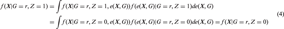
We also assume the standard strong ignorability assumption: (i) there is overlap in the propensity score distribution between the treated and control groups, that is, The propensity score balances the distribution of Matching and weighting are the two most common strategies in estimating causal effects based on propensity scores. Below we discuss propensity score matching and weighting in estimating subgroup causal effects, particularly the subgroup ATTs. In matching, for each treated unit, one finds a matched control unit from the same subgroup using propensity score as the distance metric. Within each subgroup in the matched population, the distributions of the propensity score are expected to be the same between the treated and control groups, that is, for Combining equations (2) and (3), for Hence the distribution of We now consider propensity score weighting. In estimating ATT, each treated unit is weighted by 1 and each control unit is weighted by Proposition 1


Therefore, the ATT weights balance
The subgroup ATTs can be written as
Proposition 2


The above discussions are in the setting of true propensity scores and population distributions. In observational studies, the propensity scores are usually unknown and have to be estimated from the study sample. Let

3 Subgroup balancing propensity score
Conventionally the propensity score is estimated by fitting a logistic regression model or other flexible models such as boosting
14
to the overall (full) sample. Here we use the logistic model as an example

The model is usually assessed based on some covariate balancing criterion in the overall study sample.
15
However, the estimated propensity scores often do not give exact balance in the overall sample, and the imbalance can be particularly severe in subsamples. Consequently, estimates of subgroup effects based on these estimated propensity scores may be biased. An alternative approach is to estimate the propensity score separately within each subgroup, for example, by fitting a logistic model to each subgroup sample

Matching or weighting based on the subgroup-fitted propensity scores would lead to better balance of covariates within each subgroup and thus smaller biases in causal estimates. However, due to the smaller sample sizes of the subsample, the ensuing causal estimates usually have larger variances, embodying a bias-variance tradeoff.
To address this tradeoff, we propose the SBPS as a hybrid approach to adaptively choose between the overall sample fit and the subgroup sample fit by optimizing a criterion that accounts for covariate balance for both the overall sample and the subgroup samples. Below we introduce two such criteria, one based on matching and one based on weighting.
3.1 SBPS: Matching-based criterion
When propensity score matching within each subgroup is conducted, treatment assignment can be treated as random for the overall matched population and for the matched population for each subgroup r. Hence we have the following set of moment conditions based on the standardized mean difference (SMD) measure
16
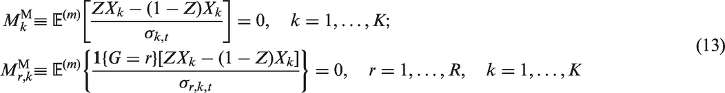
For unit i in the matched sample, let
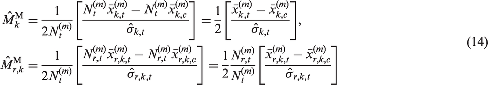
Here

We consider nearest neighbour matching with caliper 17 to remove possible bias of matching. For each subgroup r, we set the caliper to one-fourth of the standard deviation of the logit of estimated propensity scores for units in this subgroup; each treated unit in this subgroup is matched with a control unit in this subgroup whose logit of estimated propensity score is closest to and within the caliper of that of the former, and units that cannot be matched are dropped from further analysis. We allow replacement and ties in matching; hence the weights for matched treated units are all equal to one, but the weights for matched control units may be smaller or larger than one.
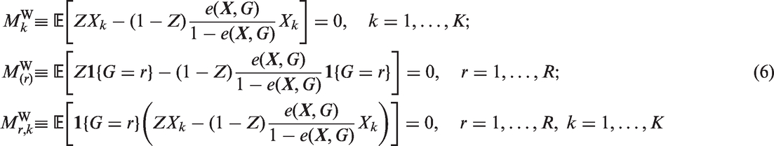
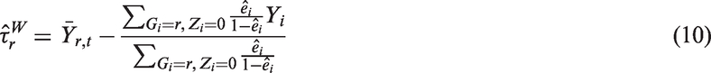
3.2 SBPS: Weighting-based criterion
The second criterion is related to covariate balance for propensity score weighting. For unit i (
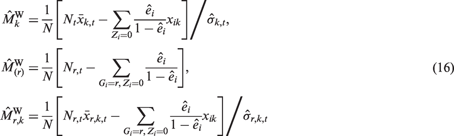
These estimates have comparable variances in a similar way to those in the matching-based criterion. The objective function is the sum of squares of these estimates, i.e.

The moment conditions for
3.3 A stochastic search algorithm to estimate the SBPS
In SBPS, for each subgroup we choose between the overall sample fit and the subgroup sample fit. Specifically, for
If R is small, we can exhaustively search through all 2
R
possible combinations for Initialize Repeat the following steps until the number of repeats is no smaller than L1, and the minimum value of the objective function encountered in the search, Randomly permutate For Repeat the following step to update If the value of FM or FW is smaller than
When R is large, results of the stochastic search algorithm depend on the random initial values and the random orders of updates for
4 Simulations
This section presents some Monte Carlo simulations to examine the performance of SPBS compared to several other methods. Consider two scenarios: (a) the number of subgroups is R = 20, and the number of units in each subgroup is N
r
= 100 ( We compare the performance of the following methods.


For CBPS, Imai and Ratkovic 7 used the “continuous updating” GMM estimator of Hansen et al. 19 which has better finite-sample properties than the usual optimal GMM estimator. However, the “continuous updating” GMM method cannot converge in one week for any of our simulations. Therefore, we use the two-step optimal GMM estimator, which is the default estimation method in the R package CBPS. We also find that the just-identified CBPS generally performs similar to or worse than the corresponding over-identified CBPS. So we only show results for the over-identified CBPS. The causal forest method does not model propensity scores and is instead an outcome-model-based approach. It directly models the outcomes and tries to identify the subpopulations with significant heterogeneous treatment effects in a data-driven fashion.
For all methods,
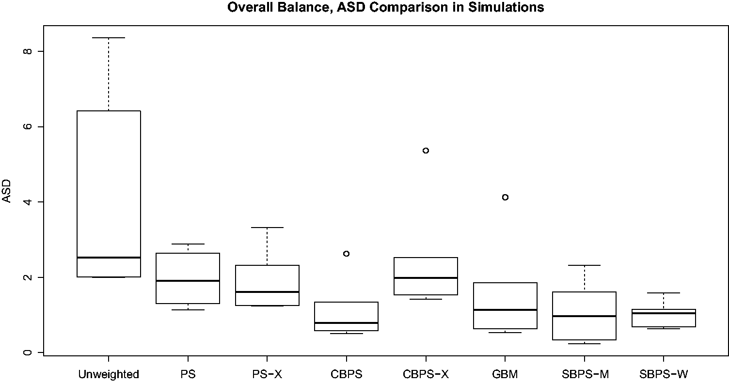
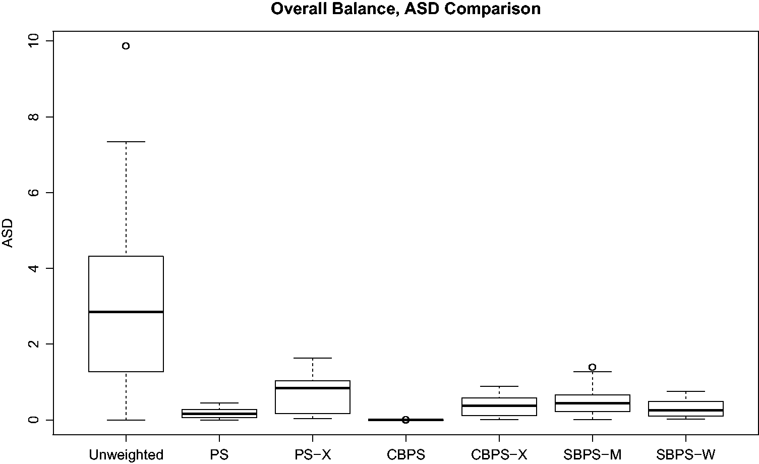
We first check the performance of the propensity score methods in balancing covariate distributions in both the subgroup samples and the overall sample. The absolute standardized difference (ASD) of X
k
in subgroup r is

Here w
i
is the weight for unit i. In the original sample, w
i
equals one for every unit. With estimated propensity scores

For the simulations with R = 20 and N
r
= 100 ( Boxplots of Boxplots of 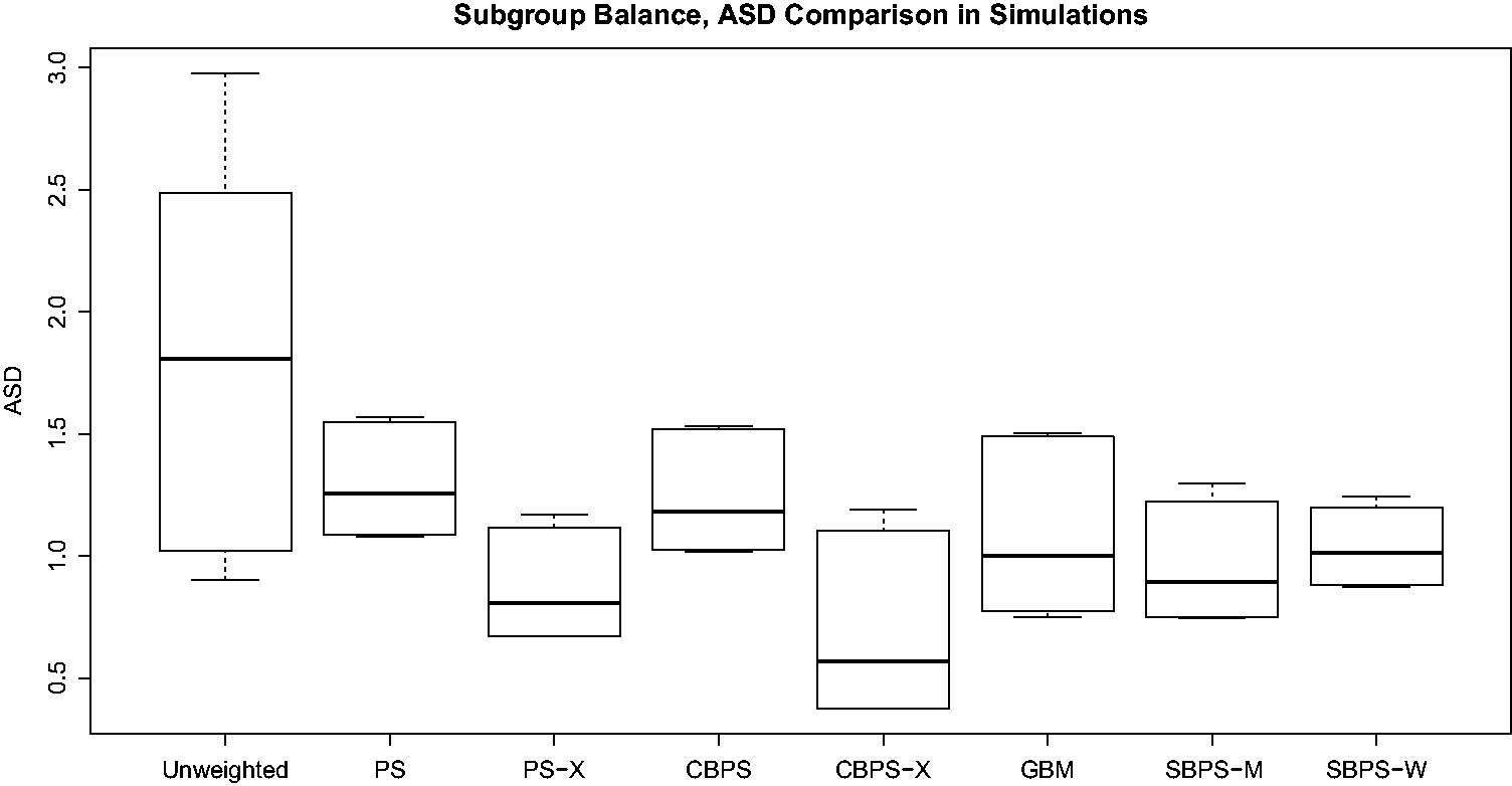
We next examine the performance of different methods in estimating subgroup ATTs. For the v'th data set, let
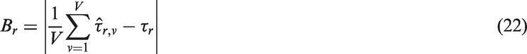
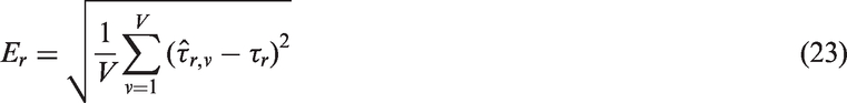
We also consider 95% confidence intervals of the form

Average performance measures of different methods using direct matching estimator
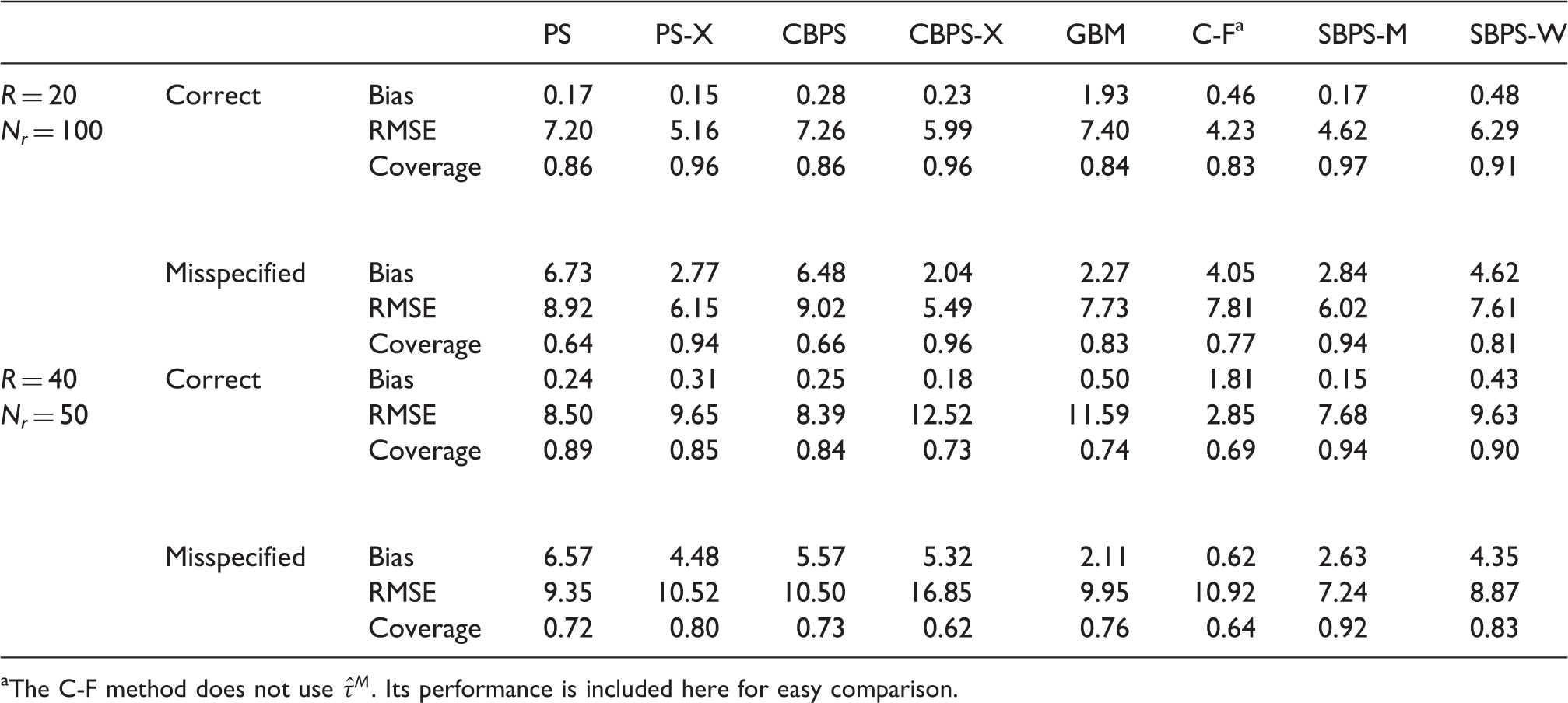
The C-F method does not use
Average performance measures of different methods using weighting estimator
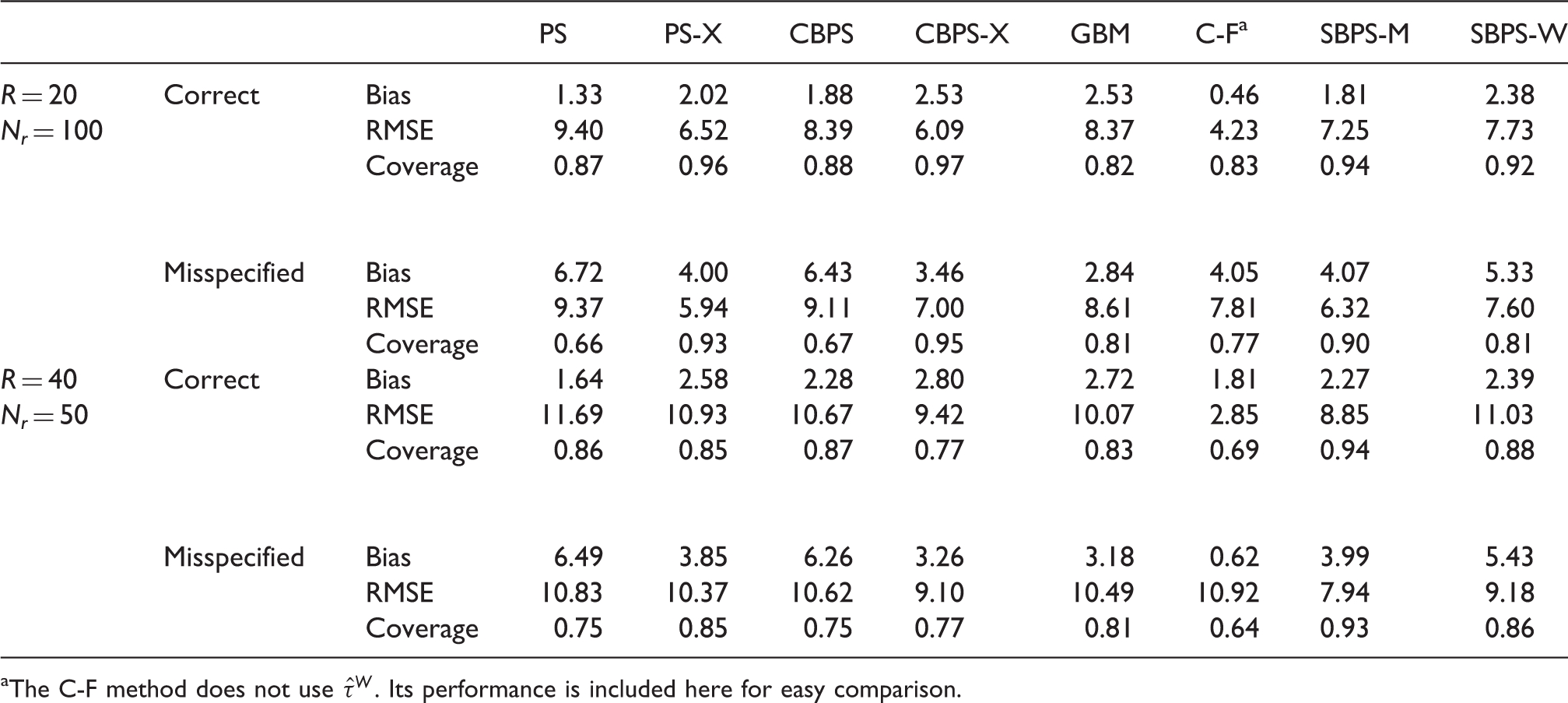
The C-F method does not use
Compared to PS, CBPS and GBM, SBPS-M has smaller average RMSE and better coverage rate, regardless of whether the model is correctly specified or misspecified. Compared to C-F, when the model is correctly specified, SBPS-M has larger average RMSE, but has much better coverage; when the model is misspecified, SBPS-M has smaller average RMSE and much better coverage. As all models are likely to be misspecified to a certain degree in real applications, SBPS-M leads to more robust results. We next compare SBPS-M with PS-X and CBPS-X. When R = 20 and N r = 100, in most cases SBPS-M has smaller RMSE, except that SBPS-M has slightly larger RMSE than CBPS-X when the model is misspecified. The coverage rates of SBPS-M and PS-X/CBPS-X are comparable. When R = 40 and N r = 50, SBPS-M has smaller average RMSE and better coverage than PS-X/CBPS-X. SBPS-W does not perform as well as SBPS-M. We recommend to use SBPS-M combined with the direct matching estimator.
For SBPS-M, if the model is correctly specified, the average proportion of subgroups using subgroup sample fit (i.e. with S r = 2) is 72.6% when R = 20 and N r = 100, and 72.0% when R = 40 and N r = 50; if the model is misspecified, the average proportion of subgroups using subgroup sample fit is 85.1% when R = 20 and N r = 100, and 81.1% when R = 40 and N r = 50. Hence in order to achieve better subgroup covariate balance, the subgroup sample fit instead of the overall sample fit is used for a fairly large proportion of subgroups.
We have also compared the performance in estimating the overall ATT using different methods (details not reported). We find that in general the SBPS method is comparable to the standard PS/CBPS, but better than PS-X/CPBS-X, GBM and C-F in estimating the overall ATT.
5 Application to the SHIW
5.1 Background
Variables in the SHIW data.
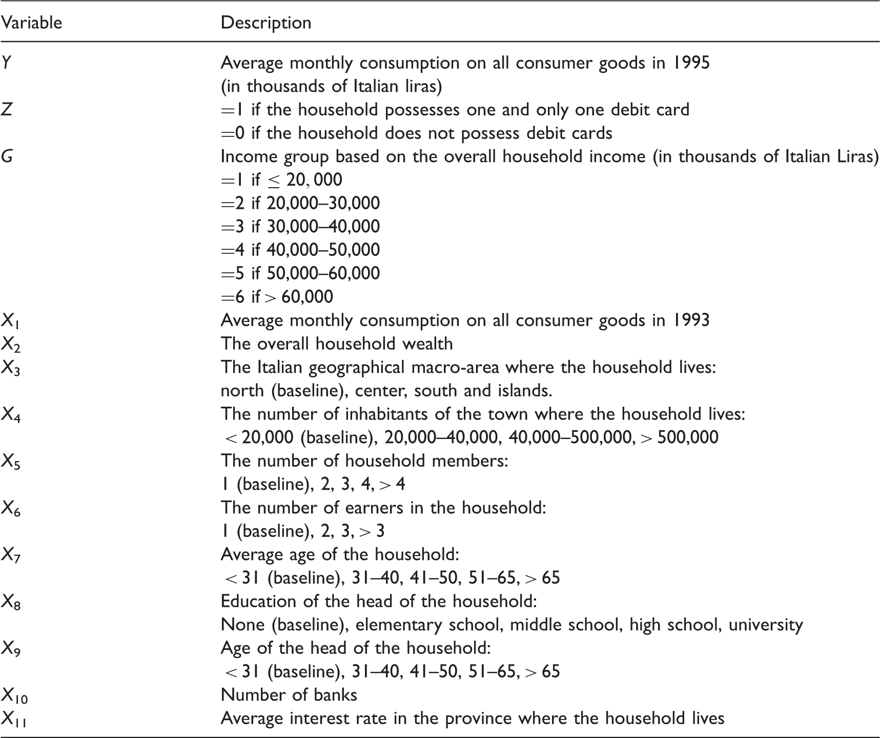
Based on the SHIW data, Mercatanti and Li 20 found statistically significant positive average effects of possessing debit cards on household spending for the whole population. The findings can be explained by the mental accounting theory which describes how consumers and their households organize, evaluate, and record their economic activities.21–23 Non-cash payment instruments, such as debit and credit cards, decouple purchases from payment and mix different purchases. Consumers have cognitive biases and hence may spend more when they use the non-cash methods.
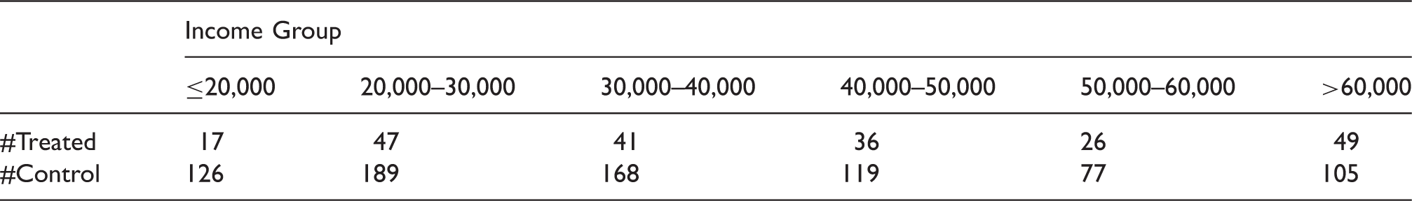
Number of treated and control units in each income group in the SHIW data.
5.2 SHIW-based simulations
We first conduct a simulation study based on the SHIW data to better understand the performance of the methods. We fix the covariates 
We conduct propensity score matching over the real data based on the estimated propensity score from fitting (11) to the real data, apply equation (25) to the matched sample, and set β0 and
We estimate the subgroup ATTs using the methods similarly as in Section 4, except that for the SBPS-M and SBPS-W methods exhaustive search is used to find the optimal combination for
Average performance measures of different methods in estimating subgroup ATTs in the SHIW-based simulations.
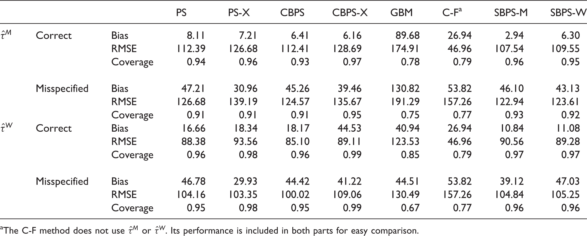
The C-F method does not use
We have also compared the performance in estimating the overall ATT using different methods (details not reported). Similar to the findings in Section 4, in general the SBPS method is comparable to the standard PS/CBPS, but better than PS-X/CPBS-X, GBM and C-F in estimating the overall ATT.
5.3 Real data analysis
For real data analysis, we excluded the GBM and C-F methods and applied the remaining six propensity score estimation methods, where for the SBPS-M and SBPS-W methods exhaustive search is used to find the optimal combination for Boxplots of Boxplots of 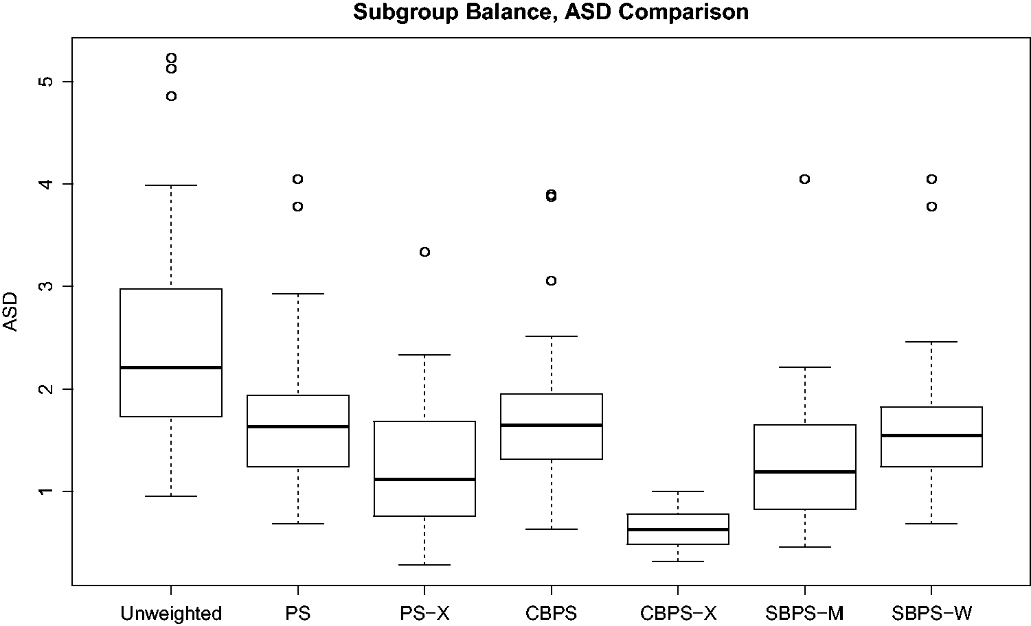
Estimated treatment effects for each income group in the SHIW data using the different propensity score estimation methods, and the associated p-values and adjusted p-values.
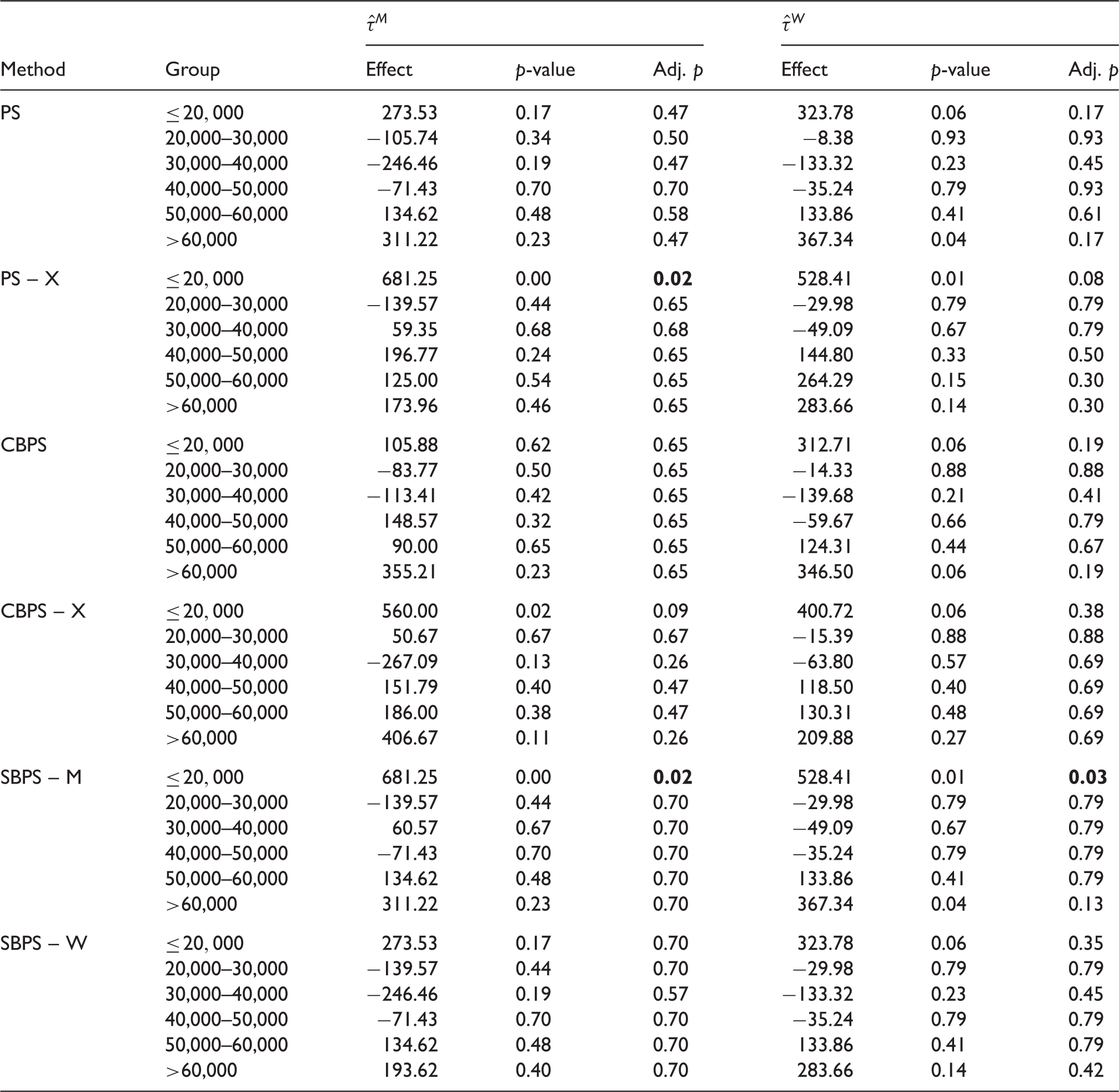
In order to account for simultaneous estimation of effects for multiple subgroups, which is known as the multiple testing issue, we use the false discovery rate method by Benjamini and Hochberg 25 to calculate the adjusted p-values in Table 6. This method controls for the false discovery rate, or the expected proportion of rejected null hypotheses that are incorrect rejections. It is more powerful than methods based on the family-wise error rate, such as the Bonferroni correction. Judging from the adjusted p-value, the PS-X method yields significantly positive effect for the lowest income group when the direct matching estimate is used, and the SBPS-M method yields significantly positive effect for the lowest income group regardless of whether the direct matching estimate or the weighting estimate is used. This is consistent with our previous conjecture.
6 Discussion
Focusing on the case where the subgroups are defined by one categorical covariate, we have demonstrated the advantage of the SBPS methods, particularly the SBPS-M method combined with direct matching estimator, compared to several existing methods in estimating subgroup treatment effects. The proposed objective functions are designed to be natural aggregate measures of the overall and subgroup-specific covariate imbalance. The subgroup variable is selected a priori by the investigators. As advocated by Kent,4,26 in comparative effectiveness research it is particularly important to stratify on the baseline risk score, also known as the prognostic score. 27 When such a risk score is available and validated from previous studies, e.g. the Framingham score in cardiovascular diseases, it is natural to perform subgroup analysis based on it.
The SBPS method can be extended to more general settings where the subgroups are defined by multiple covariates. Specifically, let G
h
(
We now use an example with two subgrouping variables to illustrate the extension of the SBPS method. Here the subgroups are defined by age and baseline risk, then the true propensity score can balance: (a) the distribution of
As the number of covariates increases, the above extension would quickly become intractable due to the rapidly increased moment balancing conditions. A possible direction is to use instead the overlap weights, 8 which weight each unit by its propensity of being assigned to the opposite group, that is, each treated unit is weighted by 1 – e and each control unit is weighted by e. Specifically, Li et al. 8 showed that when the propensity scores are estimated by maximum likelihood under a logistic regression model, the overlap weights lead to exact balance in the means of any included covariate between treatment and control groups, and the exact balance property applies to any included derived covariate, such as high order terms and interactions. Therefore, if the postulated propensity score model includes any interaction term of a binary covariate, then the overlap weights lead to exact balance in the means in the subgroups defined by that binary covariate. Considering any category variables are equivalent to a collection of binary dummy variables, we can leverage this exact balance property to subgroup analysis. For example, we can first use some high dimensional variable selection methods such as LASSO to select important interaction terms (which defines subgroups) in a propensity score model, then we estimate the propensity score using the selected main effects and interactions, finally we use these estimated propensity score to obtain the overlap weights.
In the cases of multiple subgrouping variables, a natural extension is to incorporate the potential correlation between different variables by considering a Mahalanobis-type balance metric in the objective function. Specifically, one could replace the standard deviation in our objective function (equations (14) and (15)) with the inverse of the correlation matrix of all covariates excluding the subgrouping variables. However, in the design stage, there is no guarantee that such an objective function will outperform the one with marginal moment conditions in terms of treatment effect estimation. Comparison between different balance metrics would require outcome information, which is not available in the design stage. Nonetheless, performance of such alternative balance metrics merits further investigation in empirical studies.
Much advance has been made recently in leveraging machine learning models in estimating heterogeneous treatment effects (HTE). Popular examples include the BART approach, 5 tree methods such as Causal Forest, 6 and causal boosting, 28 which are designed to identify the subpopulations with significant HTEs in a data-driven fashion. A main distinction between these methods and the proposed SBPS method is the design- versus analysis-based approach to causal inference. For example, SBPS, as well as CBPS or any propensity-score-based method, is design-based, which avoids modeling the outcome and instead focuses on ensuring covariate balance. In contrast, most of the above machine learning methods directly model the outcomes, bypassing the propensity scores and thus the balance issue. When the outcome model is correctly specified, such outcome-model-based method would produce valid and the most efficient estimates. However, the outcome model is almost always misspecified to some degree, threatening the validity of the causal conclusions. Indeed, in our simulations, the results of the Causal Forest method are generally inferior to those of SBPS in estimating the subgroup ATTs. This, of course, cannot be taken as a general evidence against the outcome-model-based methods to HTE. Rather, this highlights that comparison between the two streams (design versus analysis) of methods is highly case-dependent.
Footnotes
Acknowledgements
The authors are grateful to Peter Austin, Laine Thomas and three anonymous referees for their helpful comments that have greatly improved the exposition of this paper, and to Andrea Mercatanti for providing the SHIW data. Part of this paper was written when Jing Dong was an exchange student at Duke University under the High-Level Graduate Student Scholarship of China Scholarship Council.
Declaration of conflicting interests
The author(s) declared no potential conflicts of interest with respect to the research, authorship, and/or publication of this article.
Funding
The author(s) disclosed receipt of the following financial support for the research, authorship and/or publication of this article: Fan Li's research is partially funded by NSF-SES grant 1424688.