Experimental design and sample size considerations in longitudinal magnetic resonance imaging-based biomarker detection for multiple sclerosis

Abstract

Several modeling approaches have been developed to quantify differences in multiple sclerosis lesion evolution on magnetic resonance imaging to identify the effect of treatment on disease progression. These studies have limited clinical applicability due to onerous scan frequency and lengthy study duration. Efficient methods are needed to reduce the required sample size, study duration, and sampling frequency in longitudinal magnetic resonance imaging studies. We develop a data-driven approach to identify parameters of study design for evaluation of longitudinal magnetic resonance imaging biomarkers of multiple sclerosis lesion evolution. Our design strategies are considerably shorter than those described in previous studies, thus having the potential to lower costs of clinical trials. From a dataset of 36 multiple sclerosis patients with at least six monthly magnetic resonance imagings, we extracted new lesions and performed principal component analysis to estimate a biomarker that recapitulated lesion recovery. We tested the effect of multiple sclerosis disease modifying therapy on the lesion evolution index in three experimental designs and calculated sample sizes needed to appropriately power studies. Our proposed methods can be used to calculate required sample size and scan frequency in observational studies of multiple sclerosis disease progression as well as in designing clinical trials to find effects of treatment on multiple sclerosis lesion evolution.

Keywords

Imaging statistics sampling structural magnetic resonance imaging multi-sequence imaging neurostatistics

1 Introduction

Focal inflammatory demyelination in the central nervous system, commonly referred to as lesions, is the hallmark pathological finding in multiple sclerosis (MS). Lesion evolution is a dynamic and complex process consisting of inflammation, demyelination, tissue injury, and, in some lesions, repair that occurs over weeks to months. With the potential of a heterogeneous outcome for any given MS lesion, an imaging biomarker that can characterize differences between lesions would be of great use. Particularly, with the rapid expansion of new drugs that have the potential to impact lesion development and lesion outcomes, there is great need for an imaging biomarker that can identify differences in lesion evolution and/or outcomes for clinical trials. An ideal imaging biomarker would be sensitive to identify differences between MS lesions observed by magnetic resonance imaging (MRI). The computation of the ideal biomarker would require small number of patients given the high costs of MRI data collection. Finally, the biomarker would be identified early in lesion formation using few longitudinal MRI scans to shorten the duration of the study to limit costs and speed up the delivery to larger phase III clinical trials.

MRI is very sensitive to detecting MS lesions, but most imaging studies use MRI to find whether new lesions form or study the effects of newly forming lesions on long-term outcomes (measured months or years after lesion formation). Much fewer studies have imaged the dynamic process of MS lesion evolution as an early marker of lesion heterogeneity. Various imaging characteristics have been proposed to be useful in identifying differences in MS lesion evolution and/or outcomes including transient changes in T2-weighted signal intensity and differences in the change in the magnetization transfer ratio (MTR).^1–5 Sweeney et al.⁶ studied longitudinal intensity profiles in MS lesions using a multimodal approach with commonly available clinical sequences including T1-weighted (T1w), T2w, fluid-attenuated inversion recovery (FLAIR), and proton density-weighted (PD) sequences. More recently, Dworkin et al.⁷ built a prediction model using imaging features, clinical information, and treatment status at the time of lesion incidence to predict voxel intensities approximately a year post-incidence. However, these studies have limited applicability to clinical trials as they rely on either frequent MRIs, not commonly available MRI sequences, or study duration of one year or greater.

Many statistical methods have been developed for sample size computations in hypothesis testing.⁸ However, in serial imaging studies, traditional sample size computational approaches may not be directly applicable. Most existing sample size computation approaches focus on estimating the minimum number of patients required for a clinical trial, but do not account for the number of visits per patient and time between each visit. The problem of estimating these three parameters of interest is compounded by biological variability of lesions between and within patients, study duration, frequency of visits, and the choice of the biomarker used for a specific trial. Recent studies that calculated sample sizes for proof-of-concept trials of MS, including the study by Reich et al.,⁹ have focused on reducing one of the above factors, but were still based on the requirement of monthly MRIs scan acquisition, while more efficient methods in terms of reduced number of MRI acquisition visits were not explored.

In this paper, we develop and test experimental designs for longitudinal MRI studies in MS to identify the minimum number of MRIs needed for investigating the effects of therapeutic interventions on lesion recovery after controlling for clinical information. We use a database of structural MRI images collected from 60 patients with MS. The patients are scanned between 2000 and 2008 on a monthly basis at the National Institutes of Health Clinical Center in Bethesda, Maryland. The follow-up time is on average 2.2 years (standard deviation = 1.2) and ranges from 0.9 year to 5.5 years. First, we discuss the choice of an MRI marker that can differentiate MS lesion evolution and refer to it as lesion evolution index or index as an abbreviation. Secondly, we present methods for computing the corresponding sample sizes, considering the complex structure of the voxel level longitudinal lesion data analysis. Our proposed approach is essential for developing clinical trials where treatment effects on lesion development at voxel level are of interest.

Details of the image acquisition and preprocessing have been previously published by Sweeney et al.⁶ and are summarized here. Whole-brain two-dimensional (2D) FLAIR, PD, T2, and three-dimensional (3D) T1 volumes are acquired in a 1.5 tesla (T) MRI scanner (SIGNA Excite HDxt; GE Healthcare, Milwaukee, Wisconsin) using a body coil for transmission and a head coil as receiver. The 2D FLAIR, PD, T2 volumes are acquired using fast-spin-echo sequences, and the 3D T1 volume is acquired using a gradient-echo sequence. The PD and T2 volumes are acquired as short and long echoes from the same sequence. Medical Image Processing Analysis and Visualization (http://mipav.cit.nih.gov) and the JAVA Image Science Toolkit (http://www.nitrc.org/projects/jist) are used for image preprocessing.¹⁰ All images for each subject at each visit are interpolated to a voxel size of 1 mm³ and rigidly co-registered longitudinally and across sequences to a template space.¹¹ Extracerebral voxels are removed using a skull-stripping procedure.¹² The brain is automatically segmented using the Lesion-topology-preserving anatomical segmentation (TOADS) algorithm to produce a mask of normal-appearing white matter (NAWM)¹³ excluding white matter lesions. Since structural MRI is acquired in arbitrary units, signal intensities are normalized with respect to the average intensity of NAWM.^14,15 The normalization of the intensities allows us to compare MRI intensities among voxels within lesions and across individuals in the study.

2 Study duration and sampling in time

Subjects that failed to meet certain pre-specified inclusion criteria were excluded from the study. Specifically, we used three rules guiding subject selection: (1) the subject should have at least one new lesion during the follow-up time; (2) the subject should be scanned at least once approximately 100 days after lesion incidence; (3) all scans for the subject should pass visual quality control for segmentation of lesion tissue. As a result, 36 subjects remained in the study for further analysis. From 36 patients in the study, 21 were female and 15 were male. The baseline age of the subjects was between 18 and 60 years, with a mean of 37 years (sd = 9.6). Thirty-one patients had relapsing-remitting MS and the other five patients had secondary-progressive MS. The patients were either untreated or treated with a variety of disease-modifying therapies, including FDA-approved and experimental treatments. The treatments changed during the follow-up visits for many subjects, and hence we use time-dependent treatment indicators within each subject in building our regression models. Seven subjects also received steroids during the course of the study.

To illustrate the design of the experiments and the optimal distribution of MRI data collection over time, we use a composite MRI marker developed by Sweeney et al.⁶ We consider “lesion incidence” to be the time when the lesion is first seen on MRI (which may post-date the true biological incidence date by a time within the interval between the lesion incidence scan and the prior scan) and use intensity profiles for each lesion voxel detected at lesion incidence in the analysis. The full pipeline for extracting the longitudinal voxel-level lesion profiles from multi-sequence structural MRI is described in detail by Sweeney et al.⁶ The pipeline is divided into three main steps: (1) identifying each instance of new lesions for each study subject at baseline and all available follow-up time points, (2) temporal alignment, and (3) temporal interpolation.

Lesion incidence was obtained automatically: at baseline using the Automated Statistical Inference for Segmentation (OASIS) method¹⁶ and at each follow-up time point using Subtraction-Based Logistic Inference for Modeling and Estimation (SubLIME).¹⁷ OASIS is an automatic method for segmenting MS lesions from a combination of data from multiple modalities using logistic regression to model the probability of voxel-level lesion presence. As a result, we obtain a probability map that is thresholded to obtain a mask of lesions for each baseline image in the study. Sweeney et al.¹⁶ showed that when assessed by an experienced neuroradiologist, OASIS out-performs LesionTOADS¹⁸ in terms of estimating the lesion tissue. We use the baseline lesion masks obtained from the OASIS method to eliminate lesions present at the baseline visit, ensuring analysis of only newly incident lesions.

SuBLIME is an automatic method for identification of newly appearing lesions from MRI images of multiple modalities using logistic regression to model voxel-level MS lesion presence in subtraction images. For each follow-up scan, a subtraction image is computed by subtracting the voxel-level intensities of the previous scan from the follow-up scan. The resulting subtraction image is analyzed to obtain the map of newly appearing lesions. When we identify a new lesion by comparing the two scans, we use the time of the second scan as the incidence time. Since the SuBLIME method was used for identifying lesion incidence, only the first time when a lesion is observed was marked as lesion incidence to avoid analyzing the same lesion more than once. After selecting the lesion voxels, the intensity profiles were aligned temporally using the lesion incidence time point. Linear interpolation was used to estimate the intensities at five-day intervals. The resulting time courses were then concatenated by MRI sequences. We only included lesions with at least two follow-up scans obtained at approximately 30 ( $\pm 15$ ) days and 100 ( $\pm 15$ ) days post-incidence. As a result of these exclusion criteria, 75 lesions were removed and 561 lesions remained in our final database.

Figure 1 shows temporally registered normalized intensity trajectories of 10 randomly sampled voxels from the same lesion in T1w, T2w, PD, and FLAIR sequences, in which each curve shows the intensity profile for one voxel. The horizontal axis represents the time from lesion incidence in days, and the vertical axis represents the value of normalized signal intensities. Given that most of the transient portion of truly new lesions resolves within 10 weeks,¹ the trajectories illustrated in Figure 1 suggest that the incident lesions detected in this study were typically relatively new. Figure 2 shows the time points at which each of the 36 subjects included in the study was scanned. Each row is a subject and each point represents an MRI scan. Pink indicates the visit included newly incident lesions and blue indicates those without new lesions.

Figure 1.

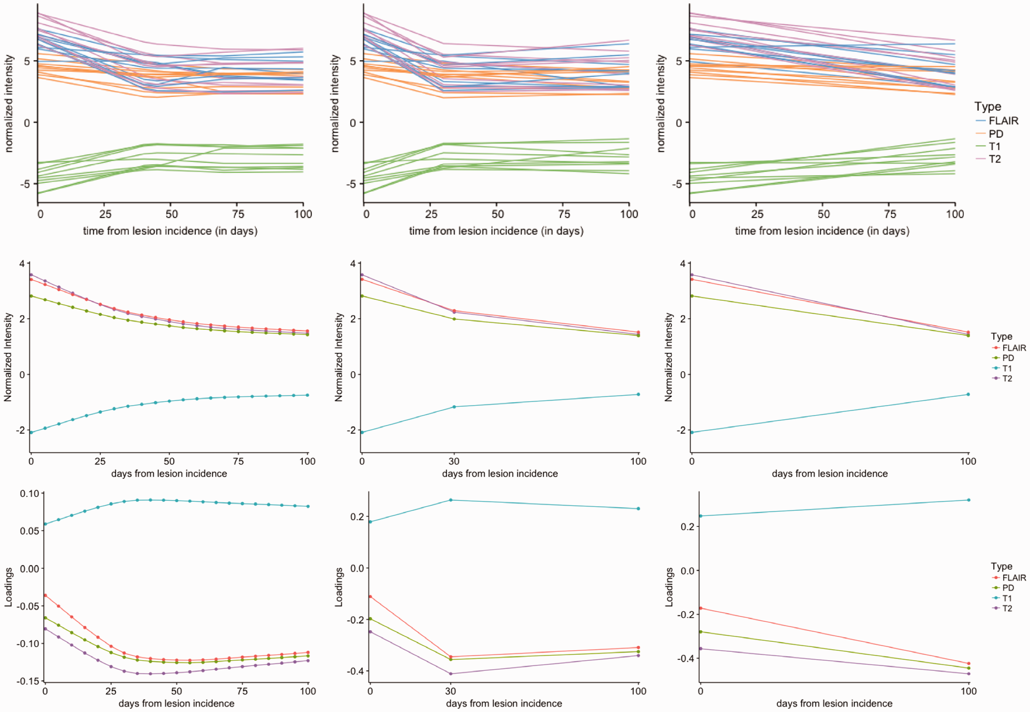
Normalized intensity trajectories (top row) for 10 randomly sampled lesion voxels in four MRI sequences. The horizontal axis shows the time in days from the lesion incidence and the vertical axis shows the normalized sequence intensities. The trajectories are after temporal alignment and linear interpolation over the 100 days after incidence, which is the time period used in this analysis. Mean intensity trajectories (second row) and loadings on the first principal component (bottom row) for Design 0, Design 1, and Design 2, from left to right. A curvature is captured by the first PC, in the opposite direction to the mean in Design 0 and Design 1. Visually, Design 1 replicated the trajectories obtained in Design 0. While Design 2 has a similar trend to Design 0, we do not observe the rapid initial response followed by a less steep change in mean and first PC trajectories in Design 0.

Figure 2.

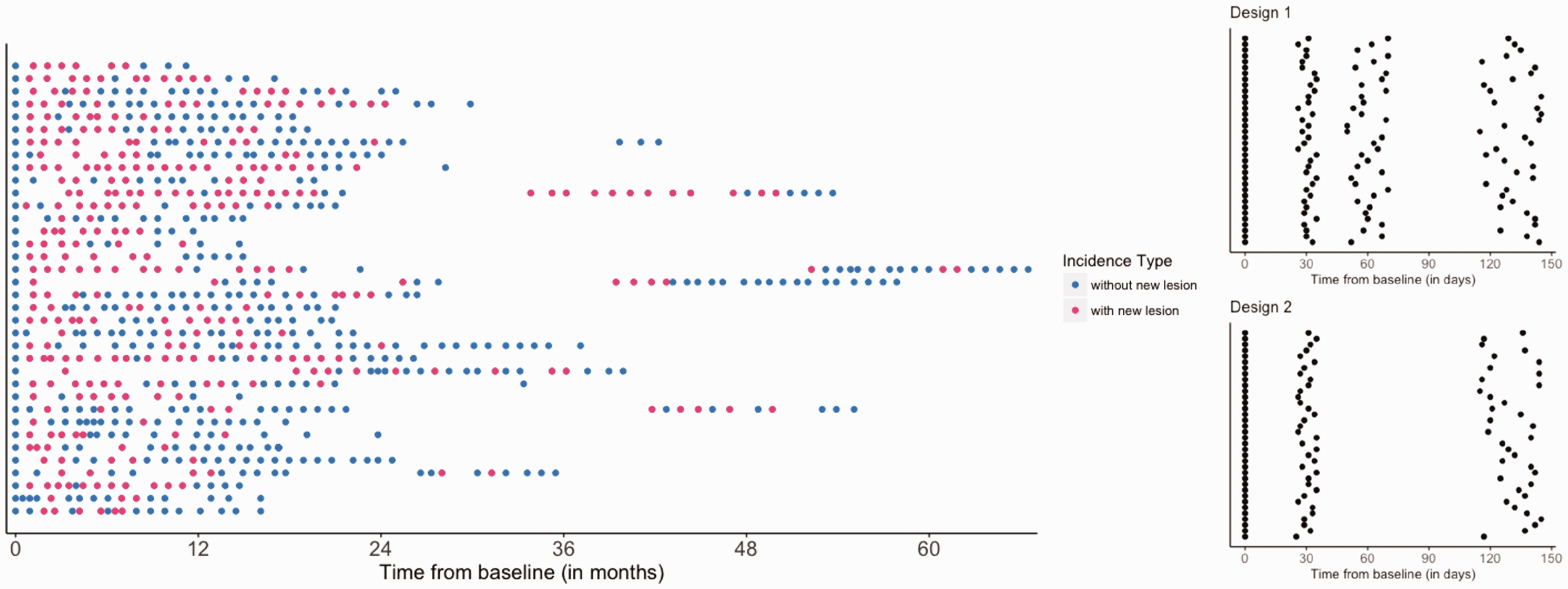
Left: Time of scan visits. Each row is a subject and each point represents an MRI scan visit. Pink indicates the visits with new lesions and blue indicates those without new lesions. Patients appear to have more new lesions at the beginning of study. Right: Sketch of the experimental design schemes for Designs 1 and 2. In both Designs 1 and 2, the newly incident lesions are identified at the second scan approximately one month after baseline scan, and have two and one follow-up scans, respectively.

We tested multiple study designs, iteratively reducing the number of MRI scans, to determine the differences in sensitivity to detect variability in evolution in new MS lesions. Figure 2 presents the design schemes considered in our study. At least two data collection visits are required to identify newly incident lesions to be used to detect lesion recovery vs. non-recovery. We present two design strategies and compare them to Design 0, which is an abridged version of a previously published study design using this MRI dataset. Sweeney et al.⁶ followed the lesions for 200 days. Design 0 is based on the assumption that five monthly MRIs are available and is similar to the study by Sweeney et al.⁶ In Design 1, we assume that one less follow-up MRI visit is conducted. In Design 2, only three MRI visits are used in the analysis, i.e. one additional MRI after lesion incidence approximately 100 (±15) days later.

3 Lesion evolution and regression analysis

We performed the following steps to estimate a biomarker of lesion evolution for each of the design schemes described in Figure 2. We extract the lesion intensity trajectories from all four sequences and estimate a voxel-specific index of lesion recovery reducing the dimension of the data while retaining important information on the variability using principal component analysis (PCA). To use the information from all four pulse sequences, we concatenate the longitudinal lesion profiles from the four sequences for each voxel. We use all follow-up scans obtained after the baseline scanning visit. For subject i, lesion l, and voxel v, let $I_{ilv} = {T 1_{ilv}, T 2_{ilv}, P D_{ilv}, FLAI R_{ilv}}$ denote the concatenated profile, where each of $T 1_{ilv}, T 2_{ilv}$ , PD_ilv, FLAIR_ilv is a $1 \times t$ vector of longitudinal intensities. Specifically, t = 3 for Design 1 and t = 2 for Design 2. After removing the mean over time from the concatenated profiles, we perform PCA on the resulting matrix. The jth entry of the intensity vector can be written as

I_{ilv} (j) = \sum_{k = i}^{K} ξ_{ilv} (k) ϕ_{k} (j)

where

ϕ_{k}

is the kth principal component (PC) and

ξ_{ilv} (k)

is the score on the kth PC for voxel v.

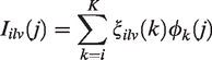
Figure 1 shows the mean profiles of the lesion trajectories and the first principal component plotted for the three study designs. The loadings on the first principal component have very similar longitudinal trends compared to the mean intensity trajectory, but in the opposite direction. In the settings of Design 1 and Design 2, the first PC explains $68 %$ and $65 %$ of the variation in the concatenated longitudinal profiles, respectively. $ξ_{ilv} (1)$ , the score on the first PC, $ϕ_{1}$ , is the voxel-level index for identifying intensity changes within lesion tissue. Positive values of $ξ_{ilv} (1)$ indicate a voxel in recovery, and negative values indicate a voxel remaining as lesion tissue. The expert validation of this index is described in detail by Sweeney et al.⁶

MRI signal intensities are normalized with respect to the average intensity of the NAWM. The normalization transforms the intensity values into units of standard deviations above or below the mean of the NAWM. The mean intensity profiles are above 0 throughout the study period for T2w, PD, and FLAIR, since lesions appear as hyperintense areas on these sequences and hence the values are larger than the average of NAWM. On the contrary, the mean intensity profile is below 0 for T1w, since lesions appear hypointense on this sequence. For T2w, PD, and FLAIR, the first principal component is negative throughout the study period and the loadings are closer to 0 at time 0, the lesion incidence. Positive scores on this PC in these sequences indicate a decrease in the intensity, corresponding to a return to an intensity value closer to that of normal-appearing tissue, i.e. lesion recovery. For T1w, the first principal component is positive throughout the study period and the loadings are also closer to 0 at the lesion incidence. Positive scores on this PC in these sequences indicate an increase in the intensity, which also correspond to a return to an intensity value of a voxel closer to that of normal-appearing tissue. To evaluate whether subsampled study designs (Designs 1 and 2), using fewer MRIs, can identify differences in the lesion evolution index we computed Pearson correlation coefficients as quantitative estimates of similarity between the estimated PC profiles at each reduced study design compared with the full study sample, Design 0. The correlation coefficient of values of the index estimated by Design 1 and Design 0 is 0.98, and the correlation between the index values estimated by Design 0 and Design 2 is 0.95. Hence, the estimated index between the reduced MRI sampled designs and analysis with the full number of scans, Design 0, is highly correlated. The high correlation between the PC scores for the three designs further illustrates that the first PC computed from each of the designs captures the relevant information concerning lesion evolution trajectory, and hence the reduced designs can be used in practice to obtain similar secondary analysis results, such as estimation of treatment effects, as those from Design 0.

From Figure 1, we observe that the estimated PC1 corresponds to the main lesion development trajectory for each of the Designs 0, 1, and 2. However, when comparing Design 2 with Designs 0 and 1, while we observe the downward trajectory of the lesion intensity profiles, we do not obtain the initial rapid decline visible in Designs 0 and 1. However, the high correlation between the lesion level PC scores indicates that for the purposes of further analysis, missing the initial rapid decline may not affect estimation of treatment effects. This observation is further confirmed by investigating the association between the estimated PC scores in Designs 1 and 2 and distance to boundary as follows.

We use visualization techniques to illustrate the relationship of the estimated index with distance of a voxel to the boundary of the corresponding lesion. We plot the distribution of the estimated PC scores by distance to the boundary. In addition, we present differences of the relationship of the index and distance to the boundary with treatment. Figure 1 shows that the first PC estimated based on data from much fewer patient visits has similar properties to that estimated using Design 0 (the design with the full set of data) in terms of longitudinal trends of the lesion estimate. Sweeney et al.⁶ showed that the degree and rate of recovery in center voxels is different from boundary voxels. We observed similar patterns of associations both in the plots based on Design 1 and those based on Design 2. In Figure 3, the curves are separated, indicating that a voxel’s score on the first principal component is associated with its distance from lesion boundary. In addition, Figure 3 shows that within the same treatment group, the voxels closer to the boundary of a lesion are more likely to have higher scores, and the voxels closer to the center of a lesion are more likely to have a lower score, consistent with the visual observation that voxels in the center of the lesion are less likely to repair. In Design 1, the average lesion index value is 1.4 (95% confidence interval (CI): –7.4, 7.0) for voxels with a distance of 1 and –4.2 (95% CI: –11.5, 3.5) for voxels with a distance of 4 or more from the boundary of the lesion. In Design 2, the average index value is 1.1 (95% CI: –5.8, 5.1) for voxels with a distance of 1 and –3.4 (95% CI: –8.9, 2.4) for voxels with a distance of 4 or more from the boundary of the lesion.

Figure 3.

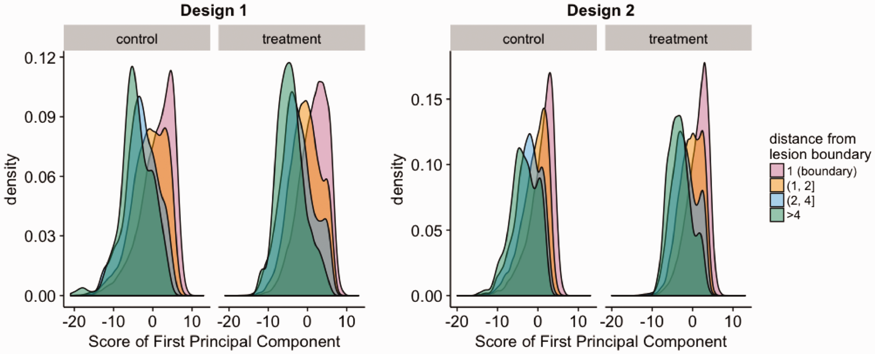
Distribution of first PC score by distance. A clear separation between curves can be observed, indicating that the distribution of the first PC score is associated with voxels’ distance from lesion boundary.

4 Association of lesion evolution index with treatment interventions

To test whether the lesion trajectory can be affected by disease-modifying treatment (after correcting for clinical covariates), we use a linear regression approach where we include random effects for subjects and lesions. The random effects for the lesions are added to take into account the longitudinal structure of the data where each subject is sampled during several visits, while the random effect for the subjects takes into account the between-subject variability.

Specifically, for each voxel v in lesion l of each subject i at each visit, we are interested in the association between the lesion evolution index and age, sex, the indicator of DMT, and the shortest distance of the lesion voxel from the boundary of the lesion of which it is a part. The treatment indicator implies treatment with any potentially DMT during the course of observation period. As we are using a longitudinal model, it is important to note that all covariates except for sex may change in value over time. Since over the course of about three months of observation, the influence of changes in age (recorded in years in our study) is likely to be relatively minor, we index this covariate by the combination of $i, l, v$ and use the value at the time of incidence. The administration of DMT also changes over the course of the study. We use the indicator of DMT at lesion incidence for each lesion in our longitudinal model as we are interested in the effect of DMT received at lesion incidence on its evolution. To account for the differences in variability structure among lesions within a subject, we also add random effects, α_i at the subject level and γ_l at the lesion level. Both random effects are assumed to follow a normal distribution: $α_{i} \sim N (0, σ_{i}^{2})$ and $γ_{l} \sim N (0, σ_{l}^{2})$ . Age is centered at the mean age of 34 years. The linear mixed-effects model can be written as follows

ξ_{ilv} (1) = β_{0} + β_{1} {Age}_{ilv} + β_{2} {Male}_{i} + β_{3} {Distance}_{ilv}

(1)

+ β_{4} {Treatment}_{ilv} + α_{i} + γ_{l} + ϵ_{ilv}

(2)

We assume the error terms are independent and identically distributed, following a normal distribution $ϵ_{ilv} \sim N (0, σ_{ϵ}^{2})$ . The variable treatment is an indicator such that ${Treatment}_{ilv} = 1$ if the subject i is receiving any disease-modifying treatment at the time of the incidence of lesion l and ${Treatment}_{ilv} = 0$ otherwise.

To estimate the precision of the estimates, we compute 95% CI for the covariate coefficients by performing parametric bootstrap. Specifically, independent and identically distributed bootstrap samples are generated from the estimated parametric model using the parameter estimates from the original data. The outline of the process is as follows

Fit the mixed effect model to the data to obtain the MLEs $\hat{β}, {\hat{σ}}_{α}^{2}, {\hat{σ}}_{l}^{2}$ , and ${\hat{σ}}_{ϵ}^{2}$ ;

Generate the bootstrap samples using the fitted model with $α_{i}^{*}, γ_{l}^{*}$ and $ϵ_{ilv}^{*}$ generated from $N (0, {\hat{σ}}_{α}^{2}), N (0, {\hat{σ}}_{l}^{2})$ , and $N (0, {\hat{σ}}_{ϵ}^{2})$ , respectively;

Fit the mixed effect model to the bootstrap data and obtain the bootstrap MLEs $\hat{β}, {\hat{σ}}_{α}^{2}, {\hat{σ}}_{l}^{2}$ , and ${\hat{σ}}_{ϵ}^{2}$ ;

Repeat steps (2)–(3) for 1000 iterations.

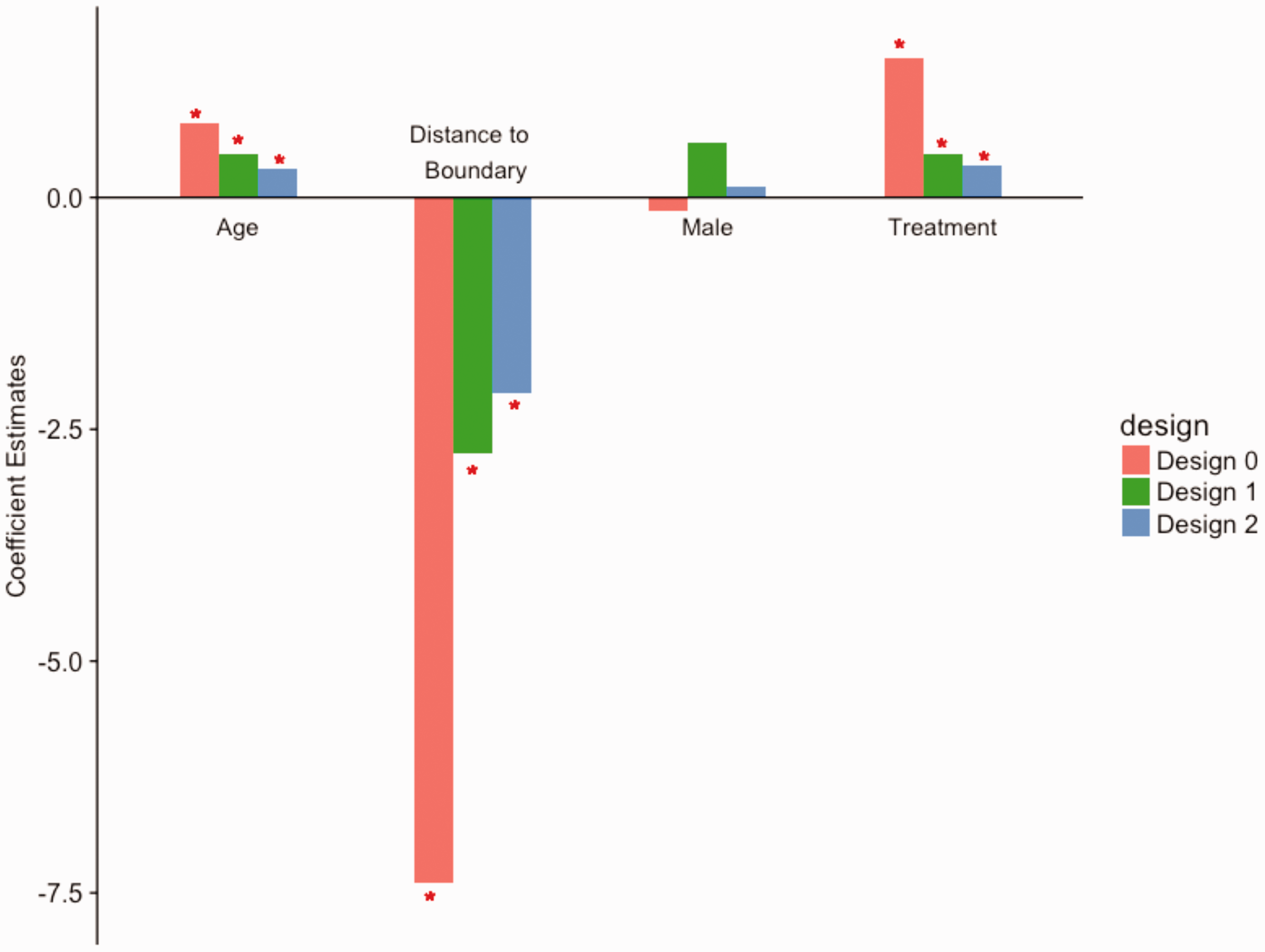
The estimates of the coefficients from fitting the multivariate mixed-effects model to explore the relationship between the lesion evolution index and the clinical covariates for all the three designs are shown in Figure 4, with asterisks indicating statistical significance at $α = 0.05$ level. The summaries of coefficient estimates, standard errors, t-values, and 95% CIs are presented in Table 1. Both Figure 4 and Table 1 indicate that for the variables that are significantly associated with the lesion recovery index, the parameter estimates are in the same direction for all three designs, except the effect sizes are relatively larger for Design 0 compared with Designs 1 and 2.

Figure 4.

Coefficients from the multivariate mixed-effects models. The bar plots show the coefficient estimates from the three designs, with asterisks indicating statistical significance at the 5% level. Both of the designs produce results that are consistent with previous study.

Table 1.

Summary of regression results for all three designs (fixed effects).

	Estimate	SE	t-Value	p-Value	95% bootstrapped CI
Design 0
Intercept	3.17	2.16	1.47	0.15	(–0.90, 7.58)
Age	0.80	0.06	14.17	<0.01	(0.69, 0.92)
Distance to boundary	–7.39	0.03	–242.79	<0.01	(–7.45, 7.33)
Male	–0.15	3.28	–0.046	0.96	(–6.36, 6.42)
Treatment	1.50	0.11	13.54	<0.01	(1.27, 1.72)
Design 1
Intercept	0.45	1.08	0.42	0.68	(–1.89, 2.50)
Age	0.47	0.02	22.37	<0.01	(0.42, 0.50)
Distance to boundary	–2.76	0.01	–256.17	<0.01	(–2.78, –2.73)
Male	0.59	1.66	0.36	0.72	(–2.70, 3.93)
Treatment	0.47	0.04	11.83	<0.01	(0.39, 0.54)
Design 2
Intercept	0.67	0.76	0.88	0.38	(–0.79, 2.06)
Age	0.31	0.02	20.17	<0.01	(0.28, 0.34)
Distance to boundary	–2.11	0.01	–260.42	<0.01	(–2.13, –2.10)
Male	–0.11	1.16	0.10	0.92	(–2.10, 2.39)
Treatment	0.34	0.03	11.56	<0.01	(0.28, 0.40)

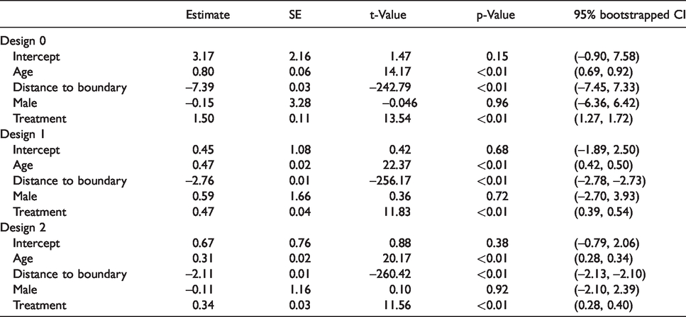
Positive values of coefficients are interpreted as higher recovery on average with an increase in the covariate. Negative values of coefficients are interpreted as higher remaining lesion tissue with an increase in the covariate. The results obtained from Design 1 and Design 2 are consistent with each other and suggest that voxels closer to the boundary have a higher chance to recover, while the voxels further away from the boundary are more likely to remain as lesion tissue, adjusting for other covariates and random effects. The results also indicate that, after adjusting for other covariates and random effects, the voxels under treatment recover better on average. The inference is consistent with the result by using Design 0.

5 Sample size and power considerations

The power of a statistical test generally depends on the sample size, effect size, and pre-defined desired level of significance.¹⁹ The goal of the analysis in this paper is to identify whether a significant difference in lesion progression index exists between a potential experimental treatment group and control group using as small a sample of participants and MRI scanning visits as possible. Hence, we are interested in testing the effect of treatment with the statistical modeling framework described in the previous section. The null hypothesis of interest is that the use of treatment does not affect the value of the index, while the alternative is that treatment leads to higher index values. Using our proposed notation, we can write the hypothesis of interest as follows

H_{0} : β_{4} = 0 vs . H_{a} : β_{4} > 0

This hypothesis can be tested using a two-sample t-test in the context of linear models. We compute the required sample size to obtain a test with a certain power (i.e. power of 80%) based on an estimated or known effect size and a pre-defined level of significance. We use the available sample data to obtain an estimate of the effect size. 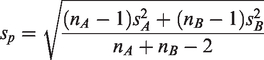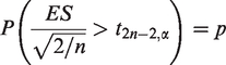Suppose the treatment group is denoted by A and the control group by B, we compute the effect size as $\frac{{\bar{X}}_{A} - {\bar{X}}_{B}}{s_{p}}$ , where $\bar{X}$ is the average value of the index and s_p is the pooled standard deviation computed as follows

s_{p} = \sqrt{\frac{(n_{A} - 1) s_{A}^{2} + (n_{B} - 1) s_{B}^{2}}{n_{A} + n_{B} - 2}}

Assuming equality of the same sample sizes of treatment and control groups, we obtain n by solving the following equality for the desired power p

P (\frac{E S}{\sqrt{2 / n}} > t_{2 n - 2, α}) = p

Due to the structure of MS data, where voxels in an MRI of the same lesion may share more similar characteristics than those of a different lesion, the power and required sample size need to be determined in a multilevel design. Such grouped data violate the assumption of independence across observations. The amount of dependence can be expressed as the intraclass correlation coefficient (ICC), defined by ρ, which is the ratio of the between-cluster variance to the total variance.²⁰ Data grouping in MS lesions resembles data clustering in cluster randomized trials, where the information gained is less than that in an individually randomized trial of the same size.²¹ Donner et al.²² proposed an approach to calculation of a sample size assuming individual randomization inflated by a Design Effect (DE), a function of cluster size and ICC, to reach the required level of statistical power under cluster randomization. Snijders¹⁹ states that the level-one sample size is of main importance for testing the effect of a level-one variable, the level-two sample size is important for testing the effect of a level-two variable, etc. The average cluster sizes are not of importance for the power of a test focusing on regression coefficients.

In order to calculate the required sample size for the full model including the random effects, $\hat{n}$ is inflated to account for clustering effects.²¹ The random effect structure of the model implies specific assumptions on the variability of the outcome within subjects and lesions. One can think of these as clusters. To offset the clustering effect, we need to multiply the estimated sample size from the fixed effects part of the model by the design effect, $1 + (r - 1) ρ$ , where r is the cluster size and $ρ$ is the ICC. We use the median number of voxels per lesion as an estimate of cluster size. We estimate the ICC by finding the proportion of variance that comes from the within-lesion variation. The population ICC is $\frac{σ_{l}^{2}}{σ_{l}^{2} + σ_{ϵ}^{2}}$ , where $σ_{l}^{2}$ denotes the variance of γ_l and $σ_{ϵ}^{2}$ denotes the variance of the noise term.

Finally, an important consideration in estimating the required sample size in this setting is the number of incident lesions between the baseline scanning visit and the first follow-up visit. One approach would be to recruit patients with markedly active disease where more incident lesions would be expected. Here, we use a data-driven approach to estimate the probability of new lesion incidence for a particular patient in the study using the observational sample we analyzed. For each patient, we can compute the probability of lesion incidence within a randomly selected month during the follow-up. By averaging these probabilities, we obtain an estimate of the probability of a randomly selected patient having at least one incident lesion at their first follow-up visit. Finally, we inflate our estimated sample size by this probability to obtain the final estimate of the sample size.

6 Sample size estimation

For both Design 1 and Design 2, we treat lesions as clusters of lesion voxels and set the cluster size as 125, which is approximately the median number of voxels in each lesion. Effect size is defined as normalized average difference in the value of lesion evolution index between treatment and control groups. The normalizing factor is the pooled standard deviation of the index values. For the same statistical power, a model with smaller effect size would require a larger sample size than one with larger effect size. ICC also affects the sample size estimation. The higher the ICC, the more lesions are needed due to the dependence-caused inefficiency of the data. The estimated ICC on the lesion level is 0.52 based on our data implying that about half of the variance comes from within-lesion variation. The effect size of treatment estimated by observational data is 0.083 for Design 1 and 0.123 for Design 2. After adjusting for clustering effect, the number of lesions required per treatment group is 834 for Design 1 and 380 for Design 2 to achieve a statistical power of 0.8. Figure 5 shows the plots of estimated sample sizes at lesion level for various effect sizes and power values. The number of patients depends on the number of lesions that each patient contributes and the lesion incidence rate.

Figure 5.

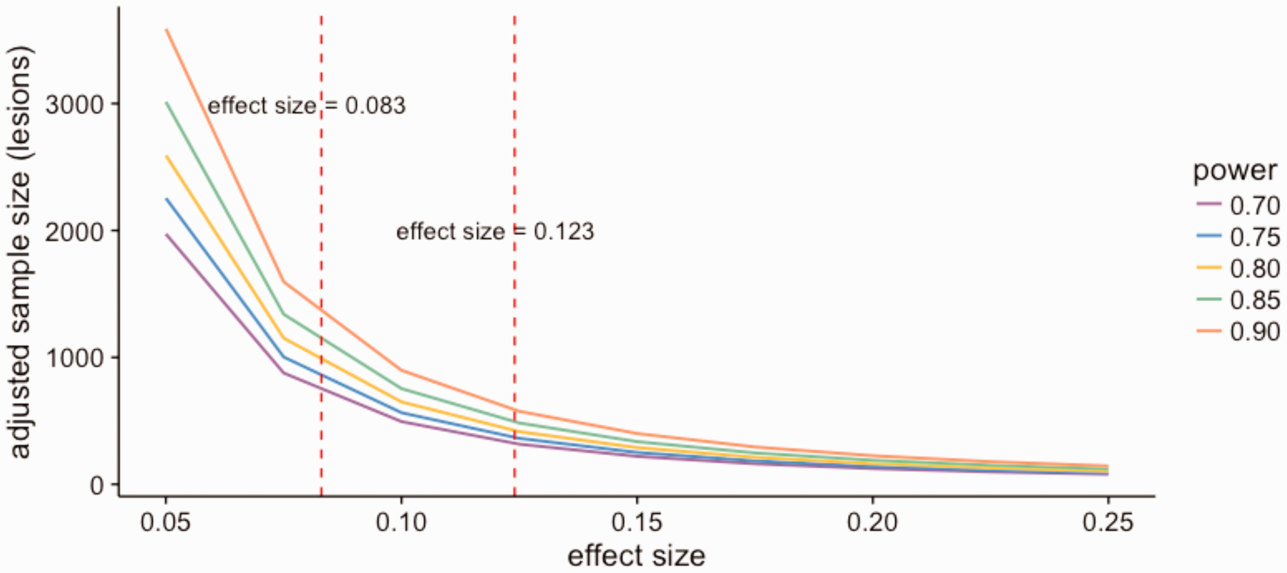
Calculated sample size vs. effect size. The sample size is adjusted for clustering effect. Estimated by observational data, the effect size is 0.083 for Design 1 and 0.123 for Design 2. Assuming there are 125 voxels in each lesion, the number of lesions required per treatment group is 834 for Design 1 and 380 for Design 2 to achieve a statistical power of 0.8.

Based on the data in this study, new lesions may not be evident at every MRI visit (see Figure 2). When new lesions were observed, an average of three new lesions was identified. However, based on our pre-specified criteria, only 60% of the subjects could be included in the analysis. Thus, there is a need to increase the calculated sample size to account for the possibility of removing data due to quality control issues and lesion incidence timing restriction.

7 Discussion

We presented experimental design strategies that can be used in MS clinical trials to identify associations of treatment interventions with lesion recovery. A lesion evolution index was computed based on multimodal clinical MRI sequences and statistical quantifying of voxel-wise lesion recovery. We described two strategies for experimental designs. By comparing two sequential MRI scans one month apart, we identified new MS lesions and observed changes in normalized signal intensity in these lesions. We showed that with as few as three MRIs, the index that quantifies lesion progression is highly correlated with one derived from full set of observations.

Using a random effects regression model, we found the use of disease modifying therapy to be positively associated with our estimated index of lesion recovery. Here we assumed that all treatments are equally effective in affecting lesion trajectories. The dataset does not lend to testing for differences between treatments, but future prospective studies could ask this important question. The positive association between voxel-level MRI intensity changes in MS lesions and therapeutic interventions after controlling for clinical information in Design 1 and Design 2 both agree with the results of a previous study.⁶ The degree of recovery in center voxels is different from boundary voxels. “distance to boundary” dwarfs the effects of other variables in Figure 4. Even though we adjusted for age and sex in multivariate regression model, there may exist unobserved differences between individuals on a treatment and those who are untreated, leading to potentially biased conclusions. The results can be validated in clinical trials that can be developed using the proposed experimental designs.

In this study, we had access to a database that contained scans from multiple visits over years for each of the participants. While having such granular data for the study participants allowed us to obtain more precise estimates of the principal component loadings of interest along with the principal component scores as biomarkers of lesion evolution. Our work shows that a similar biomarker can be obtained by a much more efficient experimental design that can be conducted in a shorter amount of time. The proposed method is data-driven and can be used as a tool for developing design strategies in other such studies if preliminary data exist for estimation of treatment effects to inform design of study visits and sample size estimation. If no preliminary data are available, the clinical trial may start with an initial small group of subjects to obtain preliminary data for building study design. In this example too, the fact that our proposed procedure can be conducted in a short amount of time is essential.

Among the 38 patients included in the analysis, only seven patients received steroids during the course of the study and only 8.5% of their lesion voxels were within 100 days post-incidence during the time they were on steroids. Due to the low steroid use in the sample of patients in our study, we decided to exclude this variable from the analysis. We identified an association between a voxel’s distance to the lesion boundary and its recovery profile. Voxels closer to the boundary are more likely to return to normal-appearing tissue, while voxels closer to the center are more likely to remain as lesion tissue.

The model was fit voxel-wise; hence, misregistration within a scan or between longitudinal scans of a subject would possibly have an effect on the performance of the model. Due to the longer interval between scans, the influence can be even greater than in previous studies with closer data collection visits. Misregistration may also affect the estimation of ICC. If there is misregistration, the voxels may appear to be less correlated to each other, leading to underestimated ICC and underestimated sample size. Since we showed a high correlation of the estimated index values obtained from the experiments with reduced number of data collection visits with that estimated using all data, we concluded that the effect of misregistration is at most small in our study. Another strength of our study is the use of data from multiple clinical MRI sequences simultaneously to obtain an estimate of lesion recovery over time. For example, newer research sequences with putative higher sensitivity to changes in myelin, such as MTR, could also be used in this study design and their added value could be evaluated.^23–25

To achieve statistical power of 80%, the calculated number of needed lesions is 834 for Design 1 and 380 for Design 2. Seemingly, Design 1 requires both more frequent visits and a larger sample size than Design 2, which may not be true in practice. Since both ICC and effect size are estimated with observational data and without CIs, these numbers are only estimates for proof-of-concept studies. Note that the estimated parameter coefficients in Designs 1 and 2 are smaller than the parameter estimates using data from Design 0; however, as their standard errors are smaller as well, the results of the hypothesis testing procedure are preserved. Considering that implementation of Design 0 may not be practical in some studies, this result shows that the subsampled designs can still be used. Previously, 315 lesions were included in analysis described by Sweeney et al.⁶ Even though the estimated sample size for subsampling designs is larger than the original study sample size, the subsampling strategy is shorter in duration and requires fewer MRI scans per person, and therefore, a more efficient study for practical reasons. Moreover, researchers can recruit more patients in earlier stages of MS, presenting with symptoms for the first time, in whom more new lesions that fit our criteria for selecting lesions may occur. However, even with these methods, the estimates of the parameters used in calculating sample sizes are often only rough and highly unreliable.²⁶ In modern studies, the sample size is not always absolutely determined in advance. For example, an adaptive design can be used, where the sample size may be influenced or controlled during the study in accordance with a pre-specified scheme.²⁷

Based on our results, we would recommend using Design 2, with one post-incidence follow-up scan, in designing experiments particularly for estimating associations of disease-modifying treatments with lesion recovery. The methods in this paper are widely applicable and can be modified to develop clinical trial designs in other studies relating MRI-based outcomes of interest with treatment and clinical information.

Footnotes

Acknowledgements

The content is solely the responsibility of the authors and does not necessarily represent the official views of the funding agencies.

Declaration of conflicting interests

The author(s) declared no potential conflicts of interest with respect to the research, authorship, and/or publication of this article.

Funding

The author(s) disclosed receipt of the following financial support for the research, authorship, and/or publication of this article: This work is supported in part by grants RO1 NS085211, R21 NS093349, and R01 NS060910 from the National Institutes of Neurological Disorders and Stroke (NINDS) and grant 5P20GM103645 from the National Institute of General Medical Sciences. The study was also partially supported by the Intramural Research Program of NINDS.

ORCID iD

Ani Eloyan

References

Meier

Guttmann

CR.

MRI time series modeling of MS lesion development.

NeuroImage 2006; 32: 531–537.

Meier

Weiner

Guttmann

CR.

MR imaging intensity modeling of damage and repair in multiple sclerosis: relationship of short-term lesion recovery to progression and disability.

Am J Neuroradiol 2007; 28: 1956–1963.

Chen

Collins

Atkins

, et al.

Magnetization transfer ratio evolution with demyelination and remyelination in multiple sclerosis lesions.

Ann Neurol 2008; 63: 254–262.

Rovira

Auger

Alonso

Magnetic resonance monitoring of lesion evolution in multiple sclerosis. Ther Adv Neurol Disord 2013; 6: 298–310.

Brown

Narayanan

Arnold

DL.

Segmentation of magnetization transfer ratio lesions for longitudinal analysis of demyelination and remyelination in multiple sclerosis.

NeuroImage 2013; 66: 103–109.

Sweeney

Shinohara

Dewey

, et al.

Relating multi-sequence longitudinal intensity profiles and clinical covariates in incident multiple sclerosis lesions.

Neuroimage Clin 2015; 10: 1–17.

Dworkin

Sweeney

Schindler

, et al.

PREVAIL: predicting recovery through estimation and visualization of active and incident lesions.

Neuroimage Clin 2016; 12: 293–299.

Gelman

Hill

Data analysis using regression and multilevel/hierarchical models. Cambridge: Cambridge University Press, 2006.

Reich

White

Cortese

, et al.

Sample-size calculations for short-term proof-of-concept studies of tissue protection and repair in multiple sclerosis lesions via conventional clinical imaging.

Mult Scler J 2015; 21: 1693–1704.

10.

Lucas

Bogovic

Carass

, et al.

The Java image science toolkit (JIST) for rapid prototyping and publishing of neuroimaging software.

Neuroinformatics 2010; 8: 5–17.

11.

Fonov

Evans

McKinstry

, et al. Unbiased nonlinear average age-appropriate brain templates from birth to adulthood. NeuroImage 2009; 47: S102.

12.

Carass

Wheeler

Cuzzocreo

, et al. A joint registration and segmentation approach to skull stripping. In: 2007 4th IEEE international symposium on biomedical imaging: from nano to macro, Arlington, VA, 12–15 April 2007, pp. 656–659.

13.

Shiee

Bazin

Ozturk

, et al.

A topology-preserving approach to the segmentation of brain images with multiple sclerosis lesions.

NeuroImage 2010; 49: 1524–1535.

14.

Shinohara

Crainiceanu

Caffo

, et al.

Population-wide principal component-based quantification of bloodbrain-barrier dynamics in multiple sclerosis.

NeuroImage 2011; 57: 1430–1446.

15.

Shinohara

Sweeney

Goldsmith

, et al. Statistical normalization techniques for magnetic resonance imaging. Neuroimage Clin 2014; 6: 9–19.

16.

Sweeney

Shinohara

Shiee

, et al.

Oasis is automated statistical inference for segmentation, with applications to multiple sclerosis lesion segmentation in MRI.

NeuroImage Clin 2013; 2: 402–413.

17.

Sweeney

Shinohara

Shea

, et al.

Automatic lesion incidence estimation and detection in multiple sclerosis using multisequence longitudinal MRI.

Am J Neuroradiol 2013; 34: 68–73.

18.

Shiee

Bazin

P-L

Cuzzocreo

, et al. Topologically constrained segmentation of brain images with multiple sclerosis lesions. Work Med Image Anal Mult Scler 2008; 71–81.

19.

Snijders

TA.

Power and sample size in multilevel modeling. Encycl Stat Behav Sci 2005; 3: 1570–1573.

20.

Maas

Hox

JJ.

Sufficient sample sizes for multilevel modeling. Methodology 2005; 1: 86–92.

21.

Rutterford

Copas

Eldridge

Methods for sample size determination in cluster randomized trials.

Int J Epidemiol 2015; 44: 1051–1067.

22.

Donner

Birkett

Buck

Randomization by cluster: sample size requirements and analysis.

Am J Epidemiol 1981; 114: 906–914.

23.

Pomann

Staicu

Lobaton

, et al. A lag functional linear model for prediction of magnetization transfer ratio in multiple sclerosis lesions. Ann Appl Stat 2016; 10: 2325–2348.

24.

Suttner

Mejia

Dewey

, et al.

Statistical estimation of white matter microstructure from conventional MRI.

Neuroimage Clin 2016; 12: 615–623.

25.

Mejia

Sweeney

Dewey

, et al.

Statistical estimation of t1 relaxation times using conventional magnetic resonance imaging.

NeuroImage 2016; 133: 176–188.

26.

Röhrig

du Prel

J-B

Wachtlin

, et al. Sample size calculation in clinical trials: part 13 of a series on evaluation of scientific publications. Deutsches Ärzteblatt International 2010; 107: 552–556.

27.

Bhatt

Mehta

Adaptive designs for clinical trials.

N Engl J Med 2016; 375: 65–74.