
Abstract
Confounding is a major concern when using data from observational studies to infer the causal effect of a treatment. Instrumental variables, when available, have been used to construct bound estimates on population average treatment effects when outcomes are binary and unmeasured confounding exists. With continuous outcomes, meaningful bounds are more challenging to obtain because the domain of the outcome is unrestricted. In this paper, we propose to unify the instrumental variable and inverse probability weighting methods, together with suitable assumptions in the context of an observational study, to construct meaningful bounds on causal treatment effects. The contextual assumptions are imposed in terms of the potential outcomes that are partially identified by data. The inverse probability weighting component incorporates a sensitivity parameter to encode the effect of unmeasured confounding. The instrumental variable and inverse probability weighting methods are unified using the principal stratification. By solving the resulting system of estimating equations, we are able to quantify both the causal treatment effect and the sensitivity parameter (i.e. the degree of the unmeasured confounding). We demonstrate our method by analyzing data from the HIV Epidemiology Research Study.
Keywords
1 Introduction
Observational studies offer an important alternative to randomized clinical trials when randomly assigning treatments to study subjects is unethical or practically impossible. 1 Analyzing data from such studies, however, confronts a difficulty that a direct comparison between the treated and untreated subjects does not necessarily reflect the causal effect of the treatment due to confounding. 2
To control for the confounding effect, study investigators typically collect a rich set of covariates with the hope that these covariates capture all background differences between treated and untreated subjects. If all background differences between the comparison groups have been correctly measured, the confounding bias can be corrected by adjustments such as multivariable regressions, stratified analyses, propensity score matching, and inverse probability weighting (IPW).3–11 Absence of unmeasured confounding (i.e. ignorability) is a strong and untestable assumption, and often implausible in observational studies.
When ignorability cannot be assumed, estimating the causal effect of a treatment and sometimes quantifying the degree of unmeasured confounding are imperative. The former is often the primary research objective, while the later becomes important when the robustness of analyses assuming ignorability needs to be objectively assessed, or when the impact of unmeasured confounding needs to be evaluated, e.g., for planning future studies in similar settings. These two objectives are typically not achievable in a single observational study, but possible given the existence of an instrumental variable (IV).
Instrumental variable methods can be traced back to 1920s,12,13 and have been extensively implemented in econometric and recently in biomedical research. Loosely speaking, an IV can be envisioned as a “randomizer” which (1) varies independent of confounders, (2) has a causal effect on treatment received, but (3) has no direct effect on the outcome of interest. These three conditions are conventionally referred to as the exogeneity, monotonicity, and exclusion restriction assumptions, respectively. 14 An IV allows for drawing causal inference about treatment effect despite the existence of unmeasured confounding. However, without additional assumptions, the IV estimate of the treatment effect applies only to a non-identifiable subpopulation of those whose treatment can be changed by the IV.15–17
The population average treatment effect (ATE) is generally of broad interest in public health and epidemiology. To infer the ATE, IVs (if available) have been used to construct bound estimates in simple settings (e.g. when both treatment and outcome are binary).18–23 In those settings, the uncertainty of unmeasured confounding effect is accounted for by a bound estimate instead of a point estimate. With continuous outcomes, obtaining bounds on ATE becomes a challenge because the domain of the outcome is typically unrestricted. In this case, additional properties of data may be implemented to construct contextually proper constraints on the observed and counterfactual data so as to identify meaningful bounds on the ATE. In this paper, we use the HIV Epidemiology Research Study (HERS)24,25 as an example to explore such constraints. Our interest is to estimate the ATE of highly active antiretroviral therapy (HAART) on patients’ CD4+ T lymphocytes (CD4) count and to quantify the degree of unmeasured confounding in the HERS.
The HIV Epidemiology Research Study was conducted when the HAART first became available to HIV-infected patients. It was a cohort study and prescription of HAART to study participants was not random. One of investigators’ interests was the initial-stage causal effect of HAART on patients’ CD4 count, an immunological marker for immune system function and disease stage. The study had collected an extensive set of covariates, but like many observational studies unmeasured confounding might still exist26,27 and its impact was unclear. To have a sense of unmeasured confounding, many HIV-positive individuals in the early HAART era were reluctant to initiate therapy due to the fear of adverse side effects and toxicity, and physicians at the time tended to prescribe HAART to patients with poor health condition, particularly those with low CD4 count. These prognostic factors were not fully measured and possibly confounded the HAART effect in a non-negligible way by affecting both treatment decisions and outcomes. 25
In this paper, we describe an approach that unifies the IV and IPW methods to simultaneously quantify (1) the ATE and (2) the degree of unmeasured confounding. To account for measured confounding, we use the IPW method 4 to “restore” the balance on measured covariates between treated and untreated subjects. To capture the unmeasured confounding, a sensitivity parameter is incorporated into the IPW estimating equations using the approach of Robins et al. 28 The sensitivity parameter is defined as the systematic difference between the treated and untreated patients if hypothetically having these patients exposed to the same treatment condition, after the measured confounding has been balanced out. This sensitivity parameter has been previously used to conduct sensitivity analyses to assess the robustness of estimated causal treatment effects to unmeasured confounding.25,29 In this paper, we assume that an IV is available. The HERS was conducted at two types of study sites: academic medical centers and community health clinics. This motivates us to consider using study site of the HERS as an instrument variable. Instead of conducting a sensitivity analysis, we take advantage of additional information provided by IV to estimate the sensitivity parameter. We propose to unify the IV and IPW estimating equations with a constraint imposed by the principal stratification 30 and contextually suitable assumptions. By solving the resulting system of estimating equations, we obtain causal bound estimates on both the ATE and the sensitivity parameter for unmeasured confounding.
The rest of the paper is organized as follows: More details about the HERS and motivations of using HERS site as an IV are provided in Section 2. Notations and models are elaborated in Section 3. In Section 4, we review the IV and IPW methods, and then introduce a unified system of estimating equations derived from them. In Section 5, we present three sets of constraints and assumptions in the context of HERS, and develop bounds on the initial-stage ATE of HAART on CD4 count and bounds on the degree of unmeasured confounding. In Section 6, we analyze the HERS data, and finally in Section 7, we offer some points for discussion.
2 The HIV Epidemiology Research Study (HERS)
2.1 Study overview
The HERS was conducted from 1993 to 2001 to investigate the natural history of HIV progression in women. Details of the study have been reported previously. 24 The study enrolled a total of 871 HIV-infected women at four study sites: Detroit, Providence, Baltimore, and New York City. Clinical outcomes (e.g. CD4 count) of each participant were recorded about every six months since enrollment. Starting around 1996, HAART became the recommended treatment regimen for HIV infected people, especially for those with low CD4 counts. 31 In this paper, we used data extracted for 201 HERS participants who completed both their seventh and eighth visits. They also met the following two conditions: (a) They were HAART naive before their seventh visit, and (b) had a low CD4 count of less than 350 cells/mm3 before their eighth visit which indicated having a deteriorating immune system. Some of them were prescribed HAART after the seventh visit. Their CD4 counts at the eight visit were used as the outcome. The study had collected a rich set of covariates, but unmeasured confounding might still exist.
Table 1 summarizes the key demographic and clinical characteristics of the 201 women. In brief, 46 women (23%) had initiated the HAART. Those receiving HAART had a higher CD4 count on average than those not on HAART, but this “as-received” treatment effect 32 was not statistically significant (standard normal z statistic = 0.58) and was certainly a biased estimate of HAART causal effect.
Summary of patient demographic characteristics by HAART receipt status and study site.
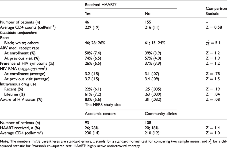
Note: The numbers inside parentheses are standard errors. z stands for a standard normal test for comparing two sample means, and
Ko et al. 25 analyzed the same data set and screened out several candidate confounders, which are listed in the upper panel of Table 1.]Notably, we found that patients receiving HAART were (a) more likely to be aware their HIV status and on antiretroviral medicines at their enrollment and at the previous visit; (b) presenting less HIV symptoms and less likely to be a drug user; (c) having higher viral loads (HIV-RNA) at their enrollment and at the previous visit; and (d) consisting of relatively more white and less black. As pointed out earlier, other confounders could likely exist and were not fully captured by the study.
2.2 HERS study site as IV
The HERS was a multi-center study and designed to recruit participants from two types of study sites for increased study generalizability. The study sites in Detroit and Providence were academic medical centers, while the other two study sites in Baltimore and New York City were community health clinics. The two types of study sites differed in many aspects. For example, the HERS investigators have noted that the academic sites had higher referral rates to the HERS by physicians and study clinic nurses and had higher HAART uptake rates among their participants. 24 Generally speaking, compared with community health clinics, academic medical centers tended to involve more actively in research on cutting-edge therapies and innovative HIV treatments besides routine patient care. As a result, physicians at the academic medical centers were more likely to be aware of the latest breakthroughs on HIV treatment, and hence when HAART first became available, they were more likely to prescribe it to HIV patients.
These differences motivate us to consider using the type of HERS study site as an IV. Using different characteristics of hospitals or physicians as IVs has been explored in other studies.27,33,34 As noted by authors of these studies, differences in health care facilities/giver can be a reasonable but not a perfect IV. In the following section, we formalize the assumptions that are needed to use HERS study site as an IV. Potential violations of these assumptions are pointed out and their impacts are discussed later in Section 7.
3 Notations and definitions
3.1 Notation
We use Z to denote an IV (in the HERS, Z = 1 if the study site is an academic medical center and
We assume that the conventional IV assumptions – the exogeneity, exclusion restriction, and monotonicity assumptions15,16 – are satisfied. The exclusion restriction implies that
3.2 Definitions of causal treatment effect
Using potential outcomes, the causal effect of a treatment can be defined at different levels. The ATE
The relationship between the ATE and LATE can be expressed using the principal stratification.
30
For a binary instrument and a binary treatment, the principal stratification suggests that the population can be partitioned into four mutually exclusive subpopulations based on the potential treatments each individual would have: In HERS,
Let us denote the estimands of ATE and LATE by 
4 Review of estimation methods
4.1 The IPW method
Putting aside the covariates for the moment, the potential outcomes can be rewritten using a marginal structural mean model6,37,38

When unmeasured confounding is absent (i.e. 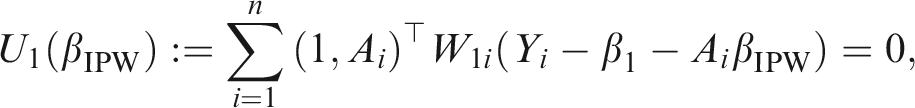
The IPW method has several properties that are worth mentioning. First, the efficiency of the resulting estimator can be improved by using stabilized weights to replace 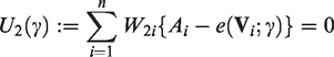
When unmeasured confounding exists, 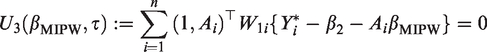

Without additional assumptions, the parameter τ is not identified by the data. The resulting estimator
4.2 The IV method
The IV methods have been widely used in econometric research.
41
In the just-identified case with a single binary IV and a binary treatment, the standard IV estimating equations are
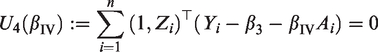
When the IV assumptions given in Section 3.1 are satisfied, the solution
Under the framework of the generalized method of moments, the IV estimating equations can be readily solved using the two-stage least squares method.14,43,44 The IV estimating equations also can incorporate a weight matrix to allow for heteroskedastic or correlated residuals, and be generalized to deal with multiple IVs and non-continuous outcomes.41,45
5 A unified system of estimating equations
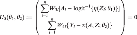
We propose to use principal stratification and the resulting constraint (1) to unify the IV and IPW methods. Specifically, we propose to jointly solve the following system of constrained estimation equations

One problem of using the constraint (1) is that
In this following, we explore and present three sets of assumptions in the context of the HERS. Each allows us to identify bounds on the ATE and unmeasured confounding parameter τ. In Sections 5.1 to 5.3, we first assume that the sample size n is sufficiently large such that the sampling variation of the estimating equations (4) is ignored. Then in Sections 5.4 and 5.5, we discuss inferences on the sampling uncertainty of bound estimates for a finite n.
5.1 Assumption on the upper limits of μ11
and μ00
The outcome variable of our interest is CD4 count, so
Assumption (A) leads to a simplified version of the Robins-Manski type bound on the ATE.18,19,23 It is straightforward to show that with known ξ0 and ξ1, the ATE falls within the interval
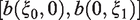
The bound on τ can be inferred by finding the values of τ such that the corresponding solutions to equation (4) are consistent with the above bound on ATE. It is straightforward to verify that for a given 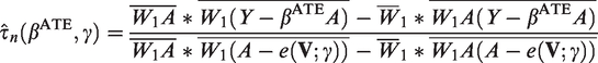

Assumption (A) alone is sufficient to identify the bounds on ATE and τ, but the two upper limits ξ0 and ξ1 need to be sufficiently large, making the two bounds too wide to be of practical value. In practices, contextually plausible constraints, such as that the average treatment effect among
5.2 Constraints on relationships between μ11
and μ00
and identified quantities
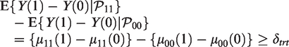
The average treatment effect among

A plausible choice for δ11 is zero; that is, we assume that on average, the subpopulation 
A negative value of δ00 implies that HAART can potentially be harmful for those who would never receive HAART at either site, while setting 3. The difference on

In the HERS, it is sensible to set The difference in average treatment effects between those who would always receive HAART and those who would never receive HAART is bounded below
For example, letting
Under this set of assumptions, it can be shown that the ATE is bounded by


5.3 Constraint conditional on measured covariates
Given the HERS data, it may be more realistic to assume that Assumption (B) holds conditional on the measured covariates
Further, we assume that the monotonicity and exclusion restriction assumptions hold conditional on
where 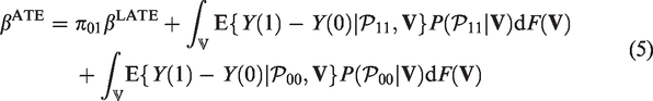
Under (B

5.4 Inference from finite samples
With a finite sample size n, we can estimate the bounds on ATE and τ, based on the results in Sections 5.1 to 5.3. We proceed by first estimating the identifiable parameters in the constraint (1). Specifically we assume two regression models

For Assumptions (A) and (B), we then estimate the function
Bounds estimates on ATE and
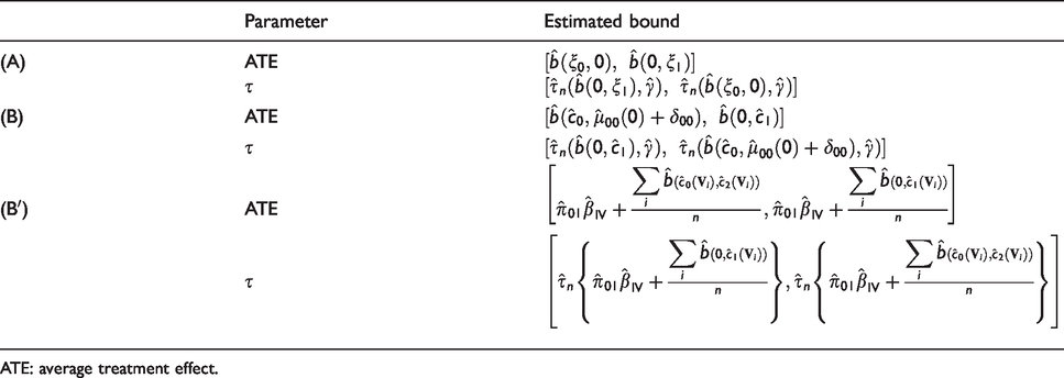
ATE: average treatment effect.
For Assumption (B Step 1. We assume two observed-data models conditional on Step 2. With the monotonicity assumption and exclusion restriction, we estimate that Step 3. We estimate the distribution of
The resulting bound estimates on the ATE and
5.5 Uncertainty region for estimated bounds
With a finite sample size, we quantify the sampling uncertainty of estimated bounds using uncertainty regions (URs), which are defined as intervals that provide a
Let 
A strong UR is an interval that contains the entire true bound 
Without assuming
6 Application to the HERS data
6.1 Preliminary analyses
The upper panel of Table 3 shows the “as-treated” (AT) effect of initial-stage HAART on CD4 count, the IPW estimate of the ATE, and IV estimate of the LATE. The AT effect is estimated by the contrast of the average CD4 counts between those actually receiving HAART and those not. The IPW uses the variables listed in Table 1 as the measured confounders
Estimates of HAART treatment effect on CD4 and
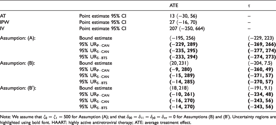
Note: We assume that
The IPW estimate suggests that at initial stage, HAART could boost patient’s CD4 count by an average of 27 cells/mm3 among all patients with a 95% CI = (
6.2 Bounds on HAART treatment effect and unmeasured confounding
We then estimate the initial-stage HAART treatment effect and the degree of unmeasured confounding using our proposed method. For Assumption (A), we let the upper limits
The lower panel of Table 3 summarizes the bound estimates of the ATE and
To obtain uncertainty regions on these bound estimates, we draw
Table 3 summarizes the point-wise, strong, and bootstrap strong 95% coverage URs. The URs under Assumptions (B) and (B
The bound estimates on
6.3 Sensitivity to unknown parameters
In this section, we conduct a simple sensitivity analysis for the unknown parameters used in the three sets of assumptions. We impose a common upper limit
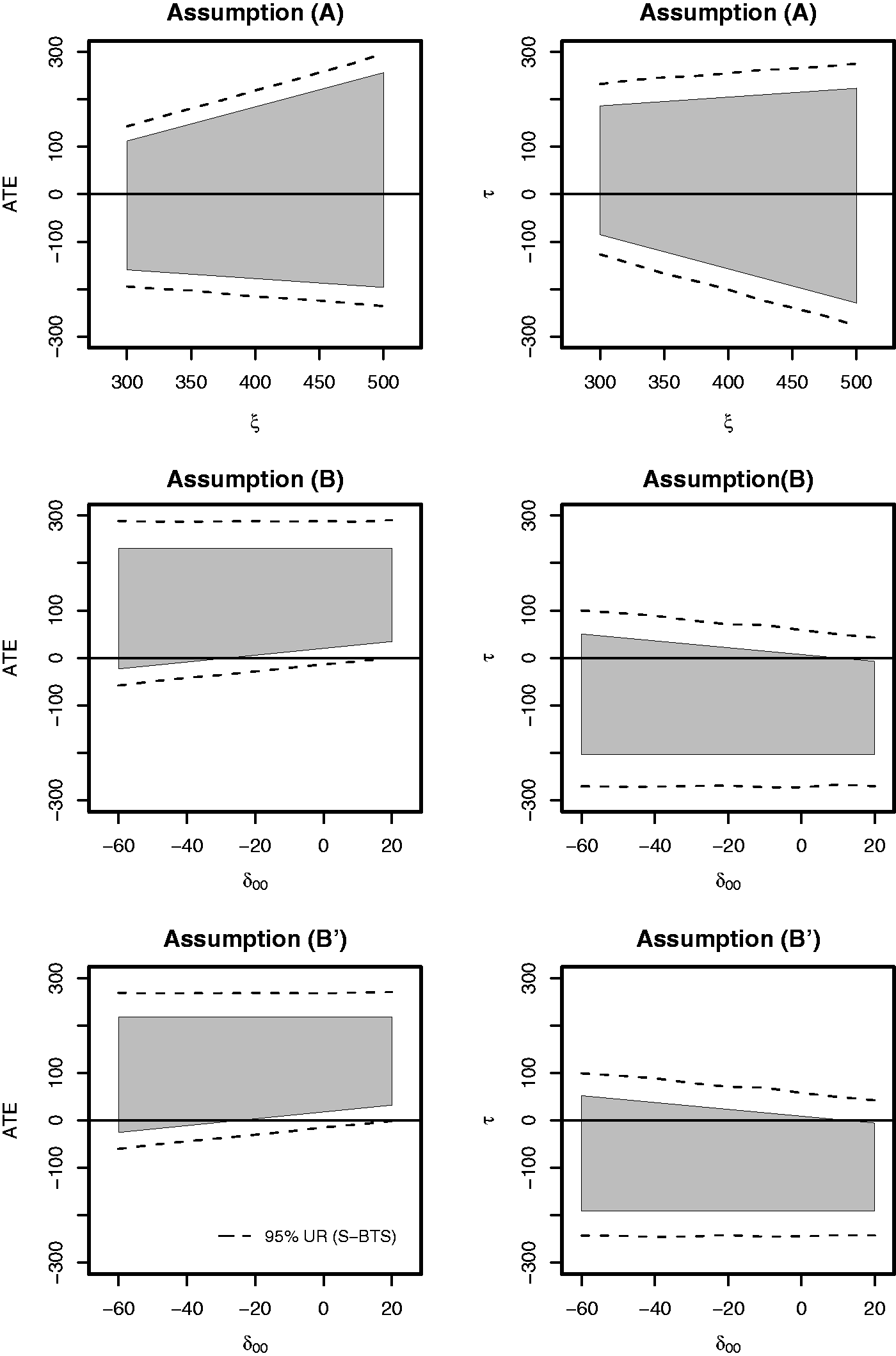
Sensitivities of bound estimates to
For (B) and (B
7 Discussions
We propose to use an IV and sets of contextually plausible assumptions to quantify the population causal effect of a treatment as well as the degree of unmeasured confounding. We describe three sets of assumptions that are suitable in an observational study (the HERS). Assumption (A) specifies the limits of the expected unobservable potential outcomes, which leads to a simplified version of the Robins-Manski bounds on ATE. Assumptions (B) and (B
Quantifying the degree of unmeasured confounding can be valuable for analysis of studies conducted in similar settings but having no IV. Several HIV observational studies
37
have been conducted contemporarily as the HERS, and could suffer from unmeasured confounding as well. In those studies when unmeasured confounding is of concern, analyses should be complemented with a sensitivity analyses as described in Section 6.3, where a plausible range for
In this paper, we use the type of study site as an instrument variable, assuming that two crucial IV assumptions (monotonicity and exclusion restriction) are satisfied. The observed HAART assignment rate at academic centers is higher than that at community clinics, an observation suggesting that the deterministic monotonicity
Moreover, replacing the deterministic monotonicity with a stochastic monotonicity52,53 assumption deserves some explorations. Roy et al.
54
assumed
The exclusion restriction could also be violated if the type of study site
There are several ways to account for the measured confounding. We use the method of inverse probability weighting by specifying a propensity score model. Alternatively, we can specify both an outcome regression model and a propensity score model and use the doubly robust (DR) estimator 8 to estimate the ATE. We do not implement the DR estimator in this paper because when unmeasured confounding exists, the DR estimator is no longer guaranteed to be consistent for ATE and could suffer more bias than other estimators. The simulations of Kang et al. 10 suggest that IPW is relatively robust to the impact of unmeasured confounding in terms of estimation bias. Because the focus issue of this paper is unmeasured confounding, we use the IPW for estimating ATE.
Finally, it should be pointed out that bound estimates may not be normally distributed asymptotically, especially when a bound occurs at the boundary of the parameter space or when the likelihood is not smooth around their true values. So practically, data analysts should check these regularity conditions in a similar way as they do when conducting statistical inference with other methods.
Footnotes
Declaration of conflicting interests
The author(s) declared no potential conflicts of interest with respect to the research, authorship, and/or publication of this article.
Funding
The author(s) disclosed receipt of the following financial support for the research, authorship, and/or publication of this article: This work was facilitated by the Providence/Boston Center for AIDS Research (P30AI042853).