Exponentially weighed moving average charts for monitoring zero-inflated proportions with applications in health care

Abstract

In the context of public health surveillance, the aim is to monitor the occurrence of health-related events. Among them, statistical process monitoring focuses very often on the monitoring of rates and proportions (i.e. values in $(0, 1)$ ) such as the proportion of patients with a specific disease. A popular control chart that is able to detect quickly small to moderate shifts in process parameters is the exponentially weighed moving average control chart. There are various models that are used to describe values in $(0, 1)$ . However, especially in the case of rare health events, zero values occur very frequently which, for example, denote the absence of the disease. In this paper, we study the performance and the statistical design of exponentially weighed moving average control charts for monitoring proportions that arise in a health-related framework. The proposed chart is based on the zero-inflated Beta distribution, a mixed (discrete-continuous) distribution, suitable for modelling data in $[0, 1)$ . We use a Markov chain method to study the run length distribution of the exponentially weighed moving average chart. Also, we investigate the statistical design as well as the performance of the proposed charts. Comparisons with a Shewhart-type chart are also given. Finally, we provide an example for the practical implementation of the proposed charts.

Keywords

Exponentially weighed moving average control chart zero-inflated Beta distribution run length average run length proportion of deaths

1 Introduction

Statistical process control (SPC) is a collection of methods that are used to monitor a process and detect changes in it. The main tool that is used for this purpose is the control chart. Initially, control charts were almost solely related to industrial processes and the detection of assignable causes that lead to an increase in the fraction of nonconforming products. Nowadays, SPC methods are not limited to industry but they are also used in a variety of scientific disciplines such as medicine, public health, finance, environment, and social networking. See, for example, Bersimis et al.,¹ Woodall² and Woodall et al.³

Mainly, there are three types of control charts: Shewhart, cumulative sum (CUSUM) and exponentially weighed moving average (EWMA) control charts. Shewhart control charts are able to quickly detect large shifts in process parameters. CUSUM and EWMA control charts (also known as control charts with memory) can quickly detect small to moderate shifts. Both are prospective methods with increased sensitivity in detecting quickly a sustained shift in the process parameters. Their superiority (compared to Shewhart charts) is attributed to the fact that they accumulate information over time. See Montgomery⁴ for a thorough introduction on control charts.

In many practical applications, especially in the areas of medicine and public health, the common approach is to monitor the counts of events (e.g. infections and deaths) either within fixed time intervals or within samples of fixed size or variable size. In the first case, the number of events is (theoretically) unbounded, taking values in ${0, 1, \dots}$ . In the second case, the number of events is upper bounded and the upper bound equals the sample size. Thus, in the first case, the usual assumption for the statistical modelling of these counts is that of the Poisson or the negative binomial distribution. Consequently, control charts based on these distributions are used for process monitoring. The $c$ -chart, a Shewhart-type chart, is a simple monitoring scheme that is applied in the case of Poisson distributed data whereas, for more efficient procedures (including those for negative binomial data), we refer to Alencar et al.,⁵ Rakitzis et al.,⁶ Rogerson and Yamada,⁷ Rossi et al.⁸ and Sparks et al.^10,9 and references therein.

In the second case, where the binomial distribution is the common model for the available (bounded) counts, a simple monitoring scheme that is applied often is the $n p$ -chart (also a Shewhart-type chart). However, instead of monitoring counts from a binomial distribution, sometimes process monitoring is based on fractions, proportions and rates. These three terms have in common that their values are (in general) on the interval $[0, 1]$ . Usually, these values are fractions of discrete variables, for example, the number of infections in a group of patients. For each individual observation (patient), we record whether a specific event is present or not. In addition, a fraction could also be a proportion. Also, there are situations (see, e.g. Ho et al.¹¹), where proportions do not result from Bernoulli experiments, such as the proportion of a drug component of a medicine, the proportion of a specific ingredient in a food product or the proportion (percentage) of body fat in patient’s body.

Traditionally, the usual $p$ -chart with the standard approach of the $3 σ$ -limits (see, e.g. Montgomery⁴) is used for monitoring proportions. The main assumption is that the number of, say, the infected patients within a sample of size $n$ , follows the binomial distribution and thus, under certain circumstances, the sample proportion follows (approximately) a normal distribution. It goes without saying that in real problems this approximation is questionable most of the time. Moreover, the $n p$ - and $p$ -charts cannot be applied in cases where the proportions do not result from Bernoulli experiments. It is known that the binomial distribution is skewed to the right when the success probability $p < 0.5$ . Thus, for processes with a low in-control (IC) proportion $p_{0}$ the normal approximation is not valid, unless the sample size at each sampling stage is very large. Consequently, in cases like this, the $p$ -chart has an increased false alarm rate (FAR). In industry, these processes are characterised as high-quality processes (see, e.g. Ali et al.¹² and references therein) whereas, in a medical context, these processes are related to rare health-events.

The problem of monitoring a Bernoulli process and the respective ‘success’ probability $p$ has been studied by several researchers. There are several works on CUSUM and EWMA charts for monitoring proportions; see Aytaçoğlu and Woodall,¹³ Daryabari et al.,¹⁴ Joner Jr et al.,¹⁵ Neuburger et al.,¹⁶ Reynolds and Stoumbos,¹⁷ Rossi et al.,¹⁸ Sego et al.,¹⁹ Spliid²⁰ and Weiß and Atzmüller²¹ and references therein. Szarka and Woodall²² provided an extensive review that covers a wide variety of methods. However, all the above-mentioned methods are applicable only in the case of proportions that are results from Bernoulli experiments.

A way to provide a unified solution that can be used for process monitoring, when the available data are (in general) in $[0, 1]$ , is to use the Beta distribution as the theoretical model that describes the stochastic behaviour of the sample proportions (individual values in $[0, 1]$ ). Also, this choice overcomes the problem of the actual distribution of the sample proportion, without resorting to questionable approximations or approximations with requirements difficult to meet. This can be attributed to the fact that it is a very flexible continuous distribution, having a large variety of shapes (see also Kieschnick and McCullough²³). Bury²⁴ stated that the Beta distribution can be used to model data in $(0, 1)$ , that is, any real number between zero and one but neither zero nor one.

Gupta and Nadarajah²⁵ presented a number of applications of the Beta distribution and it seems that these authors are the first who considered an application using control charts. Sant'Anna and ten Caten²⁶ used Shewhart control charts based on the Beta distribution to monitor fraction data, as an alternative method for monitoring proportions (instead of the $p$ chart).

It is not unusual in medical and health-related applications the occurrence of an excessive number of zeros. Each zero is related to, for example, the absence of the (health) event. Consequently, on the data that are available from health-related processes, there will be percentages, fractions or rates equal to zero. Under this perspective, we expect to monitor data in the range $[0, 1)$ and the Beta distribution is not an appropriate model. Therefore, we seek for a mixed (discrete-continuous) distribution to model $[0, 1)$ data.

Recently, de Araujo Lima-Filho et al.²⁷ studied upper one-sided Shewhart-type control charts based on the zero-one-inflated Beta distribution of Ospina and Ferrari.²⁸ Also, the authors considered cases where there is an excessive number of zeros in the data and developed Shewhart charts based on the zero-inflated Beta (BEZI) distribution. In the case of control charts for attributes data (or counts data, which are realizations from a discrete probability distribution, such as the Poisson or the binomial distribution), zero-inflated models have become popular as more appropriate models when there is an excessive number of zeros in the data. For an up-to-date review of the area, see Mahmood and Xie.²⁹ It is worth mentioning that with the term attributes we refer to quality characteristics that cannot be conveniently represented numerically (e.g. smoker/non-smoker, infected/not infected, etc.). Usually, these characteristics are classified into two or more categories, with the most common classification (in a broad sense) being that of ‘conforming’ and ‘nonconforming’, according to the specifications of these characteristics. Further details on control charts for attributes can be found in Montgomery.⁴

So far, only Shewart-type charts have been studied in the case of Beta and zero-inflated Beta distribution. As already said, Shewhart charts are not sensitive in the detection of small shifts in the process mean level. Therefore, in this paper, we study in detail the EWMA chart for monitoring proportions of health-related events when there is an excessive number of zero values in the data. The chart is based on the BEZI distribution and we will refer to it as the BEZI-EWMA chart. As a memory-type chart, it is expected to have better performance than the corresponding Shewhart chart in the detection of small and moderate shifts in process parameters. In addition, it needs to be investigated if the performance of the BEZI-EWMA chart is affected by the presence of zeros, especially when the number of zeros is excessively high. Even though the CUSUM chart is more popular in health-related applications, the EWMA control charts have also been occasionally used in public health surveillance, especially in detecting disease outbreaks.^10,30

The outline of the paper is the following. In Section 2, we provide in brief the properties of the BEZI distribution. In Section 3, we present the Shewhart and EWMA charts based on the zero-inflated Beta distribution. In Section 4, we provide the results of an extensive numerical study, regarding the performance of the BEZI-EWMA chart. We present also comparisons between the Shewhart and the EWMA charts for BEZI processes. An example of the use of the proposed charts is given in Section 5. Finally, in Section 6, we give some conclusions, recommendations and topics for future research. The details on the Markov chain method that is used for the computation of the run length (RL) properties of the BEZI-EWMA chart are given in the Appendix.

2 The zero-inflated Beta distribution

The Beta distribution is a flexible continuous distribution that can be used to model fractions, proportions and characteristics that take values in the interval $(0, 1)$ . The probability density function (pdf) of a random variable (rv) $W$ following the standard Beta distribution $Beta (u_{1}, u_{2})$ is given by

f_{Beta} (w | u_{1}, u_{2}) = \frac{Γ (u_{1} + u_{2})}{Γ (u_{1}) Γ (u_{2})} w^{u_{1} - 1} (1 - w)^{u_{2} - 1}

(1)

where

0 < w < 1

u_{1} > 0

u_{2} > 0

and

Γ (u) = \int_{0}^{\infty} x^{u - 1} e^{- x} d x

is the Gamma function at point

u > 0

. The mean and the variance of the Beta distribution are, respectively, given by

E (W) = \frac{u_{1}}{u_{1} + u_{2}}, Var (W) = \frac{u_{1} u_{2}}{(u_{1} + u_{2})^{2} (u_{1} + u_{2} + 1)}

Ferrari and Cribari-Neto³¹ proposed a re-parametrization of the pdf given in equation (1) offering an attractive simplification. Let

μ = \frac{u_{1}}{u_{1} + u_{2}} and ϕ = (u_{1} + u_{2})

(2)

Then the pdf, the mean and the variance of the Beta distribution

Beta (μ, ϕ)

are, respectively, equal to

f_{Beta} (w | μ, ϕ) = \frac{Γ (ϕ)}{Γ (μ ϕ) Γ ((1 - μ) ϕ)} w^{μ ϕ - 1} (1 - w)^{(1 - μ) ϕ - 1}, 0 < w < 1

(3)

E (W) = μ and Var (W) = \frac{μ (1 - μ)}{(1 + ϕ)}

(4)

where

μ \in (0, 1)

is the mean of

W

. Also,

ϕ

is known as the precision parameter since it can be used to control the variance of

W

. From equation (4) we deduce that as

ϕ

increases, the variance of the

Beta (μ, ϕ)

distribution decreases.

As already mentioned, fractional data, rates and proportions may (in general) have values in the interval $[0, 1]$ . Therefore, the Beta distribution cannot be used to model data of that kind. A more suitable model is that of the BEZI distribution.²⁸ The pdf and the cumulative distribution function (cdf) of an rv $W$ following the BEZI distribution with parameters $μ$ , $ϕ$ and $ν$ (i.e. $W \sim BEZI (μ, ϕ, ν)$ ) are, respectively, equal to

\begin{aligned} f_{BEZI} (w | μ, ϕ, ν) & = {\begin{matrix} ν, & if w = 0 \\ (1 - ν) f_{Beta} (w | μ, ϕ), & if 0 < w < 1 \end{matrix} \end{aligned}

(5)

F_{BEZI} (w | μ, ϕ, ν) = ν I_{[0, 1]} (w) + (1 - ν) F_{Beta} (w | μ, ϕ), w \in R

(6)

where

ν \in (0, 1)

is the probability that

W = 0

f_{Beta} (w | μ, ϕ)

and

F_{Beta} (w | μ, ϕ)

are the pdf and the cdf of the Beta distribution defined in Ferrari and Cribari-Neto³¹ with

μ \in (0, 1)

and

ϕ > 1

. Note also that

ν

is the inflating (or mixture) parameter of the BEZI distribution while

I_{A} (x)

is the indicator function, which equals one if

x \in A

and zero otherwise. Moreover, the mean and the variance of

W

are, respectively, equal to

E (W) = μ (1 - ν) and Var (W) = (1 - ν) (\frac{μ (1 - μ)}{(1 + ϕ)} + ν μ^{2})

(7)

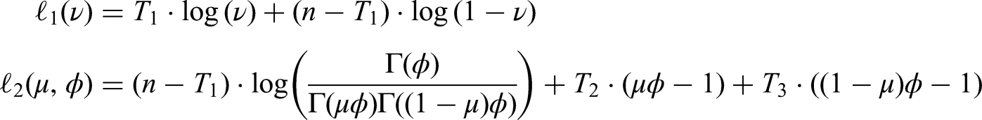
Let $W_{1}, W_{2}, \dots, W_{m}$ be a random sample from a $BEZI (μ, ϕ, ν)$ distribution. Then, using the maximum likelihood estimation (MLE) method, the estimates $\hat{μ}$ , $\hat{ϕ}$ , and $\hat{ν}$ are obtained by maximizing numerically the log-likelihood function $\log (L (θ))$ , which is given by (see Ospina and Ferrari²⁸)

ℓ (θ) = \log (L (θ)) = ℓ_{1} (ν) + ℓ_{2} (μ, ϕ)

where

θ = (μ, ϕ, ν)

and

\begin{aligned} ℓ_{1} (ν) & = T_{1} \cdot \log (ν) + (n - T_{1}) \cdot \log (1 - ν) \\ ℓ_{2} (μ, ϕ) & = (n - T_{1}) \cdot \log (\frac{Γ (ϕ)}{Γ (μ ϕ) Γ ((1 - μ) ϕ)}) + T_{2} \cdot (μ ϕ - 1) + T_{3} \cdot ((1 - μ) ϕ - 1) \end{aligned}

with

T_{1} = \sum_{i = 1}^{m} I_{{0}} (w_{i})

T_{2} = \sum_{i : w_{i} \in (0, 1)} \log (w_{i})

and

T_{3} = \sum_{i : w_{i} \in (0, 1)} \log (1 - w_{i})

. The summation for

T_{2}

and

T_{3}

is made for all

w_{i}

values in the sample (

i = 1, 2, \dots, m

) that are

> 0

and

< 1

. Then,

\hat{ν} = T_{1} / m

, while the MLE

\hat{μ}, \hat{ϕ}

μ, ϕ

can be found only numerically. Note also that the maximum likelihood estimates of

θ

are directly computed with R³² by using the package gamlss.³³

3 Control charts for monitoring a BEZI process

In this section, we present a Shewhart and an EWMA chart for monitoring a BEZI process. For the rest of the paper, we assume that when the process is IC, process parameters equal $μ_{0}$ , $ϕ_{0}$ , and $ν_{0}$ . Therefore, the proposed charts are suitable for monitoring the process in real-time, or for a Phase II analysis, as it is sometimes called the real-time monitoring of a process. During Phase II analysis, the values of the process parameters are known. In this work, we assume that they have been obtained from previous studies or they have been accurately estimated from an IC preliminary sample that has been collected from the process. The estimation of the IC values of the process parameters is the purpose of the Phase I analysis. During the Phase I analysis, the control chart is applied retrospectively on the process and the aim is to determine the values of the process parameters as well as the control limits that will be used during Phase II analysis. Further details on the difference between Phase I and Phase II can be found in Montgomery.⁴ When assignable causes are present (i.e. out-of-control process (OOC)), then at least one of the parameters has shifted to an OOC value $μ_{1}$ , $ϕ_{1}$ and $ν_{1}$ , that is, $μ_{1} \neq μ_{0}$ and/or $ϕ_{1} \neq ϕ_{0}$ and/or $ν_{1} \neq ν_{0}$ .

For shifts in $μ$ and $ν$ , we assume that $μ_{1} = δ μ_{0}$ and $ν_{1} = τ ν_{0}$ , for $δ \in (0, 1 / μ_{0})$ and $τ \in (0, 1 / ν_{0})$ . When $δ = τ = 1$ , the process is IC. We denote as $μ_{0, W}$ the IC process mean, which is given by equation (7) for $μ = μ_{0}$ and $ν = ν_{0}$ . In a similar manner, for $μ = μ_{1}$ and $ν = ν_{1}$ , we obtain the OOC process mean $μ_{1, W}$ . Also, it is worth mentioning that for $δ \in (0, 1)$ and $τ = 1$ or for $τ \in (0, 1)$ and $δ = 1$ it is $μ_{1, W} < μ_{0, W}$ and a decrease has occurred in the process mean level. On the other hand, for $δ \in (1, 1 / μ_{0})$ and $τ = 1$ or for $τ \in (1, 1 / ν_{0})$ and $δ = 1$ it is $μ_{1, W} > μ_{0, W}$ and an increase has occurred in the process mean level.

Note also that in this work we will not consider shifts in $ϕ$ and thus we simply assume that $ϕ_{0} = ϕ_{1} = ϕ$ . The aim in practise is to detect changes in the process mean level $μ_{0, W}$ , which is actually the IC value of the proportion under study. From equation (7) we see that changes in $ϕ$ do not affect its value.

3.1 BEZI-Shewhart chart

Next, we present a Shewhart chart with probability limits for monitoring a BEZI process. Further details can be found in de Araujo Lima-Filho et al.²⁷ Let $α$ be the desired FAR. Also, we assume that when the proportions are results of Bernoulli experiments, at each sampling stage $i \geq 1$ , we collect a sample of size $n_{i}$ and then we compute the value $W_{i} = X_{i} / n_{i}$ , where $X_{i}$ is the number of events (e.g. deaths) in a sample of size $n_{i}$ (e.g. patients). Otherwise, if proportions are not results of Bernoulli experiments, at sampling stage $i \geq 1$ , we record a value $W_{i} \in [0, 1)$ , which is plotted on the chart. For example, the percentage of alcohol in a patient’s body where the zero value denotes its absence. For both cases, we assume that $W_{i}$ follows a BEZI distribution.

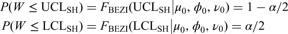
Then, by using the distribution of proportion $W$ (introduced in Section 2), we setup the BEZI-Shewhart control chart. This chart can detect shifts in either parameter $μ$ or $ν$ of a BEZI model. Here, the aim is to detect increasing shifts on the process mean level. Generally speaking, for a given FAR $α$ and equal tail probability limits, the upper control limit ${UCL}_{SH}$ and the lower control limit ${LCL}_{SH}$ of a BEZI-Shewhart chart are determined by the following equations:

\begin{aligned} P (W \leq {UCL}_{SH}) & = F_{BEZI} ({UCL}_{SH} | μ_{0}, ϕ_{0}, ν_{0}) = 1 - α / 2 \\ P (W \leq {LCL}_{SH}) & = F_{BEZI} ({LCL}_{SH} | μ_{0}, ϕ_{0}, ν_{0}) = α / 2 \end{aligned}

where

F_{BEZI} (\cdot | μ_{0}, ϕ_{0}, ν_{0})

is the cdf of the BEZI distribution, in the case of an IC process. Moreover, following the proposal in de Araujo Lima-Filho et al.,²⁷ if the probability

ν_{0}

for zero value is

ν_{0} \geq α / 2

, then only an upper control limit has to be determined. In that case,

{UCL}_{SH}

is given by

P (W \leq {UCL}_{SH}) = F_{BEZI} ({UCL}_{SH} | μ_{0}, ϕ_{0}, ν_{0}) = 1 - α

(8)

Next, we proceed only with

{UCL}_{SH}

Clearly, from (8) we deduce that ${UCL}_{SH} = F_{BEZI}^{- 1} (1 - α | μ_{0}, ϕ, ν_{0})$ , where $F_{BEZI}^{- 1} (\cdot | μ_{0}, ϕ, ν_{0})$ is the inverse cdf of the BEZI distribution for an IC process. Once the ${UCL}_{SH}$ is determined, successive observations ( $W_{i}$ values) from the BEZI process are plotted on an upper one-sided control chart that signals if a proportion is greater than the upper control limit, that is, when for the first time $W_{i} > {UCL}_{SH}$ . This is an indication of an increase in the true proportion of the events.

3.2 BEZI-EWMA chart

The EWMA control chart³⁴ for monitoring the proportion of health-related events uses the following EWMA statistic

Z_{i} = λ W_{i} + (1 - λ) Z_{i - 1}, i = 1, 2, \dots

(9)

where

W_{i}

is the sample proportion at each sampling stage,

Z_{0} = μ_{0, W} \equiv μ_{0} (1 - ν_{0})

and

0 < λ \leq 1

is the smoothing parameter. The context is the same as for the case of the BEZI-Shewhart chart. The BEZI-EWMA chart gives an OOC signal at sample

i \geq 1

Z_{i} < LCL

or if

Z_{i} > UCL

where LCL and UCL are the lower and the upper control limits of the chart. Both limits are placed symmetrically in distance

L

(in standard deviation units) from the IC process mean level, that is

UCL / LCL = μ_{0, W} \pm L σ_{0, W} \sqrt{λ / (2 - λ)}

(10)

Note also that the limits given in (10) are also known as steady-state EWMA limits (see, e.g. Human et al.³⁵) The UCL and LCL values (or, equivalently, the

λ

and

L

) are properly selected through a design study so that the BEZI-EWMA chart has the desired FAR and it is sensitive enough in the detection of specific shifts in process parameters. If for the given values of

λ

and

L

, the

LCL < 0

, then it is set equal to zero. Consequently, the chart is upper-sided and can only detect increases in the process mean level.

According to Sparks,³⁶ the EWMA statistic (see equation (9)) can be viewed as a weighted average of all the observed data from the beginning of process monitoring, which are available at time point $i$ . This is the reason why it is able to detect moderate and persistent shifts in the monitoring process. The EWMA chart has the advantage that it is easy to interpret and can be optimised by selecting the appropriate values for $λ$ and $L$ when the IC parameter value $μ_{0, W}$ is known and the shifts $δ$ and/or $τ$ are known, as well.

3.3 Performance of control charts

Control charts are evaluated by the properties of their RL distribution. The RL is defined as the number of points plotted on the chart until it triggers for the first time an OOC signal. For example, for the BEZI-EWMA chart, the $R L$ is defined as

RL = min {i \geq 1 | Z_{i} \notin [LCL, UCL]}

where UCL and LCL are given in (10).

In the case of the upper one-sided BEZI-Shewhart chart, the $RL = min {i \geq 1 | W_{i} > {UCL}_{SH}}$ and it is a geometric rv, since it expresses the number of points plotted on the chart (i.e. the number of trials) until the chart gives an OOC signal for the first time (i.e. until the first success). Its parameter (success probability) is $p_{out} = P (W_{i} > {UCL}_{SH}) = 1 - F_{BEZI} ({UCL}_{SH} | μ, ϕ, ν)$ . Therefore, the pdf and the cdf of RL are defined for $l = 1, 2, \dots$ and they are equal to

f_{RL} (l) = p_{out} (1 - p_{out})^{l - 1}, F_{RL} (l) = 1 - (1 - p_{out})^{l}

Consequently, the average RL (ARL) of the upper one-sided BEZI-Shewhart chart equals

ARL = 1 / p_{out}

, the standard deviation of the run-length distribution (SDRL) equals

SDRL = \sqrt{1 - p_{out}} / p_{out}

while, the

γ

-percentile point

{RL}_{γ}

(

γ \in (0, 1

)) of RL, is given by

{RL}_{γ} = ⌈ \frac{\ln (1 - γ)}{\ln (1 - p_{out})} ⌉

where

⌈ \dots ⌉

denotes the rounded-up integer. For

γ = 0.5

, we obtain the 0.5-percentile point

{RL}_{0.5}

or the median RL (MRL). Clearly, when

(μ, ϕ, ν) = (μ_{0}, ϕ_{0}, ν_{0})

the

p_{out} = α

, where

α

is the FAR of the chart and hence, all RL-based metrics are referred to the IC case. When

(μ, ϕ, ν) = (μ_{1}, ϕ_{1}, ν_{1})

, the

p_{out} = 1 - β

, where

β

is the type-II error of the chart and hence, all RL-based metrics are referred to the OOC case.

The computation of the RL properties of the BEZI-EWMA control chart is feasible through the use of the Markov chain methodology, which was originally proposed by Brook and Evans³⁷ (see also Bersimis et al.,³⁸ Fu and Lou³⁹ and Saccucci and Lucas⁴⁰ and references therein). Further details can be found in the Appendix.

For $λ = 1$ , the BEZI-EWMA chart coincides with the BEZI-Shewhart chart of de Araujo Lima-Filho et al.²⁷ Also, for $λ = 1$ and $ν = 0$ , the BEZI-EWMA chart coincides with the Beta chart of Sant'Anna and ten Caten.²⁶ Moreover, given $λ, L$ and for $ν = 0$ , the BEZI-EWMA chart is the Beta-EWMA chart, which is a memory-type chart for monitoring proportions following a Beta distribution. After some necessary modifications, the same methodology that is described in this work can be used for studying a Beta-EWMA chart. Further details are left to the readers.

4 Numerical study

In this section, we present the results of an extensive numerical study, regarding the performance of the BEZI control charts. When the process operates at the IC state, the ARL (SDRL) will be denoted as ${ARL}_{0}$ ( ${SDRL}_{0}$ ) while in the case of an OOC process, it will be denoted as ${ARL}_{1}$ ( ${SDRL}_{1}$ ). Given the values of $μ_{0}$ , $ϕ_{0}$ and $ν_{0}$ and the values for the design parameters of each chart (i.e. ${UCL}_{SH}$ or $(λ, L)$ ) the ${ARL}_{0}$ has a specific value.

Next, we assume two possible types of shifts in process parameters: one shift on $μ$ and one shift on $ν$ . More specifically, we assume that when the process operates in an OOC state, $μ_{1} = δ μ_{0}$ , $δ > 1$ or $ν_{1} = τ ν_{0}$ , $0 < τ < 1$ . When exactly one of these two shifts occurs, the mean $μ_{0, W}$ (see equation (7)) of the BEZI process shifts from the IC value $μ_{0, W} = μ_{0} (1 - ν_{0})$ to an OOC value $μ_{1, W} > μ_{0, W}$ , where either $μ_{1, W} = δ μ_{0} (1 - ν_{0})$ or $μ_{1, W} = μ_{0} (1 - τ ν_{0})$ . As already said, we assume that the precision parameter equals $ϕ$ and remains unchanged. Note also that in the work of de Araujo Lima-Filho et al.,²⁷ the authors did not consider separate shifts in each of the process parameters but they just considered an additive shift in the IC process mean level.

For a fair comparison (in terms of ARL) between the different control charts, we have to set the IC ARL at the same pre-specified value. Then, given the values for $μ_{0}$ , $ϕ_{0}$ , $ν_{0}$ and ${ARL}_{0}$ , we determine the values of the design parameters of each chart. Clearly, for the upper one-sided BEZI-Shewhart chart, ${UCL}_{SH} = F_{BEZI}^{- 1} (1 - \frac{1}{{ARL}_{0}} | μ_{0}, ϕ, ν_{0})$ . For the determination of the design parameters $(λ, L)$ of the BEZI-EWMA chart, the related procedure is as follows:

Step 1. Choose the values for $ϕ$ , $μ_{0}$ , $ν_{0}$ and ${ARL}_{0}$ .

Step 2. Choose the value of $λ \in (0, 1)$ and determine the unique $L$ value that gives an IC ARL value equal to ${ARL}_{0}$ .

In general, small values for $λ$ are recommended, with common values being in the interval $[0.05, 0.30]$ . In this work, we choose $λ$ to be one of the values ${0.05, 0.10, 0.20, 0.30}$ . Then, for each $λ$ , we determine $L$ value with a three decimals accuracy (for faster convergence of the implemented algorithms) so that the IC ARL value equals the target ${ARL}_{0}$ value.

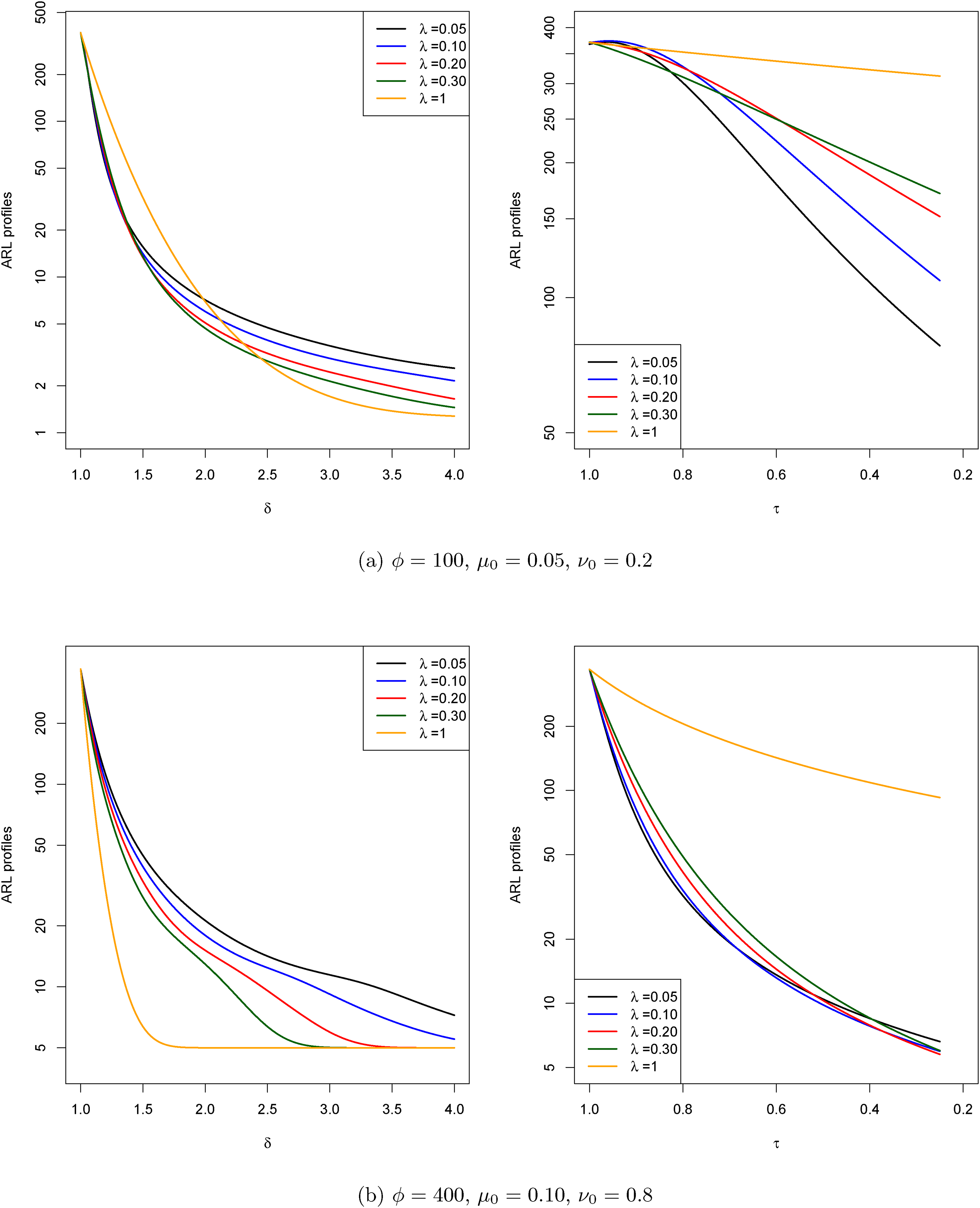
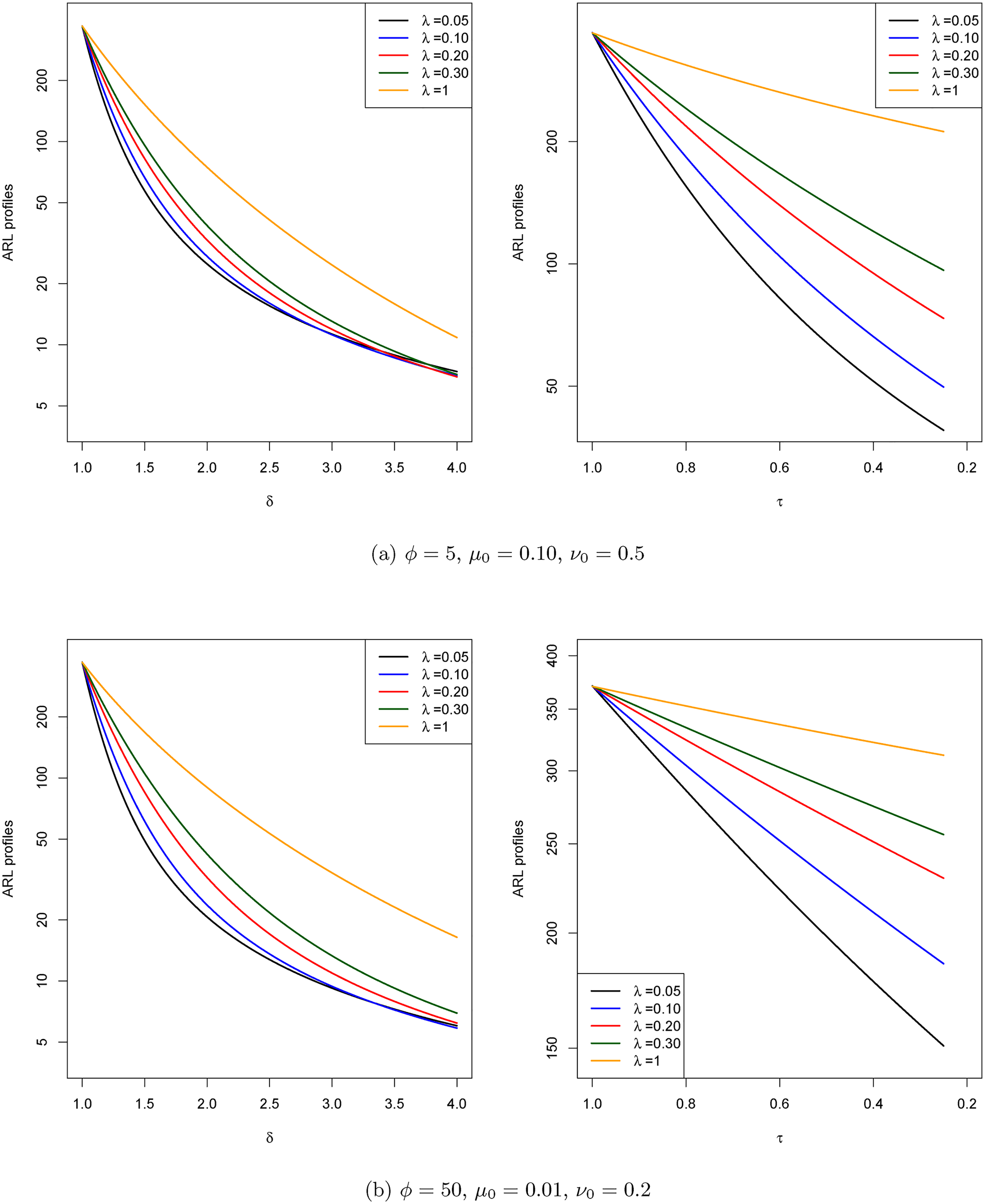
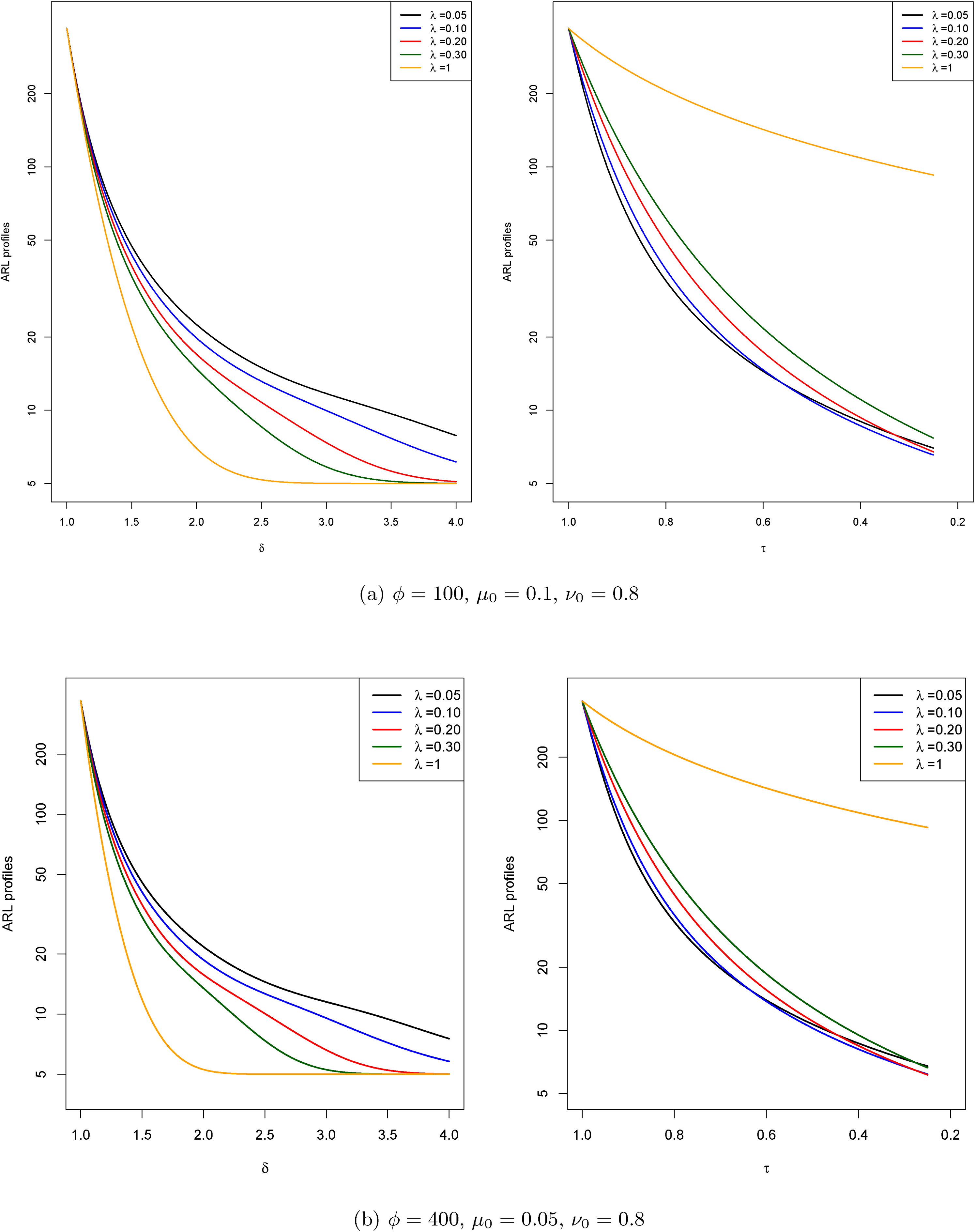
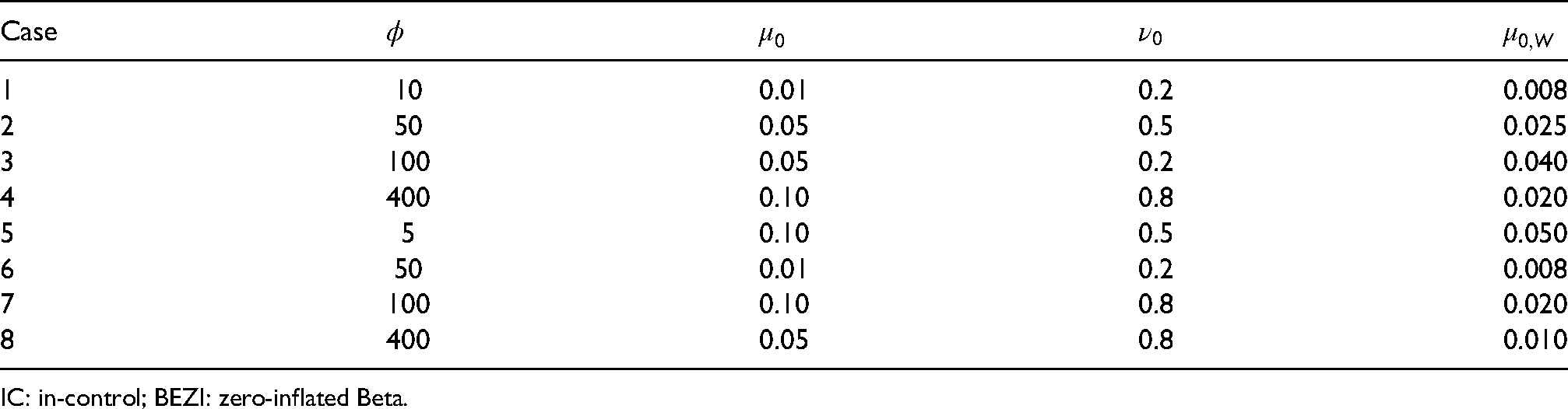
Next, we present the findings of an extensive numerical study regarding the statistical design and performance of the BEZI-Shewhart and the BEZI-EWMA charts. We consider several IC BEZI processes with different levels of zero-inflation as well as different levels of precision (in terms of $ϕ$ ). In the complete numerical study, we considered $ϕ \in {5, 10, 50, 100, 400}$ , $μ_{0} \in {0.01, 0.05, 0.1}$ and $ν_{0} \in {0.2, 0.5, 0.8}$ . The aim is to examine the performance of the charts under various BEZI processes and assess the impact of the parameters and the different shifts on $δ$ and $τ$ . The IC process mean level is $μ_{0} (1 - ν_{0})$ and varies from 0.002 to 0.08. Due to space economy, we only present in Figures 1 to 4 eight different IC scenarios (cases), regarding the $A R L$ performance of the charts. These scenarios are given in Table 1, in the column ‘Case’. All charts have the same IC ARL value ${ARL}_{0} \approx 370.4$ . For shifts only in $μ_{0}$ , we considered $δ \in [1, 4]$ and $τ = 1$ , while for shifts only in $ν_{0}$ , we considered $τ \in [0.25, 1]$ and $δ = 1$ . For the same scenarios, we evaluated the performance of the Shewhart and EWMA charts in terms of the OOC measures SDRL, MRL and ${RL}_{0.95}$ . However, due to space economy, the respective figures are given in the Supplemental material. Also, the lines in Figures 1 to 4 for $λ = 0.05, 0.10, 0.20, 0.30$ refer to the respective BEZI-EWMA charts, while the line $λ = 1$ refers to the upper one-sided BEZI-Shewhart chart.

Figure 1.

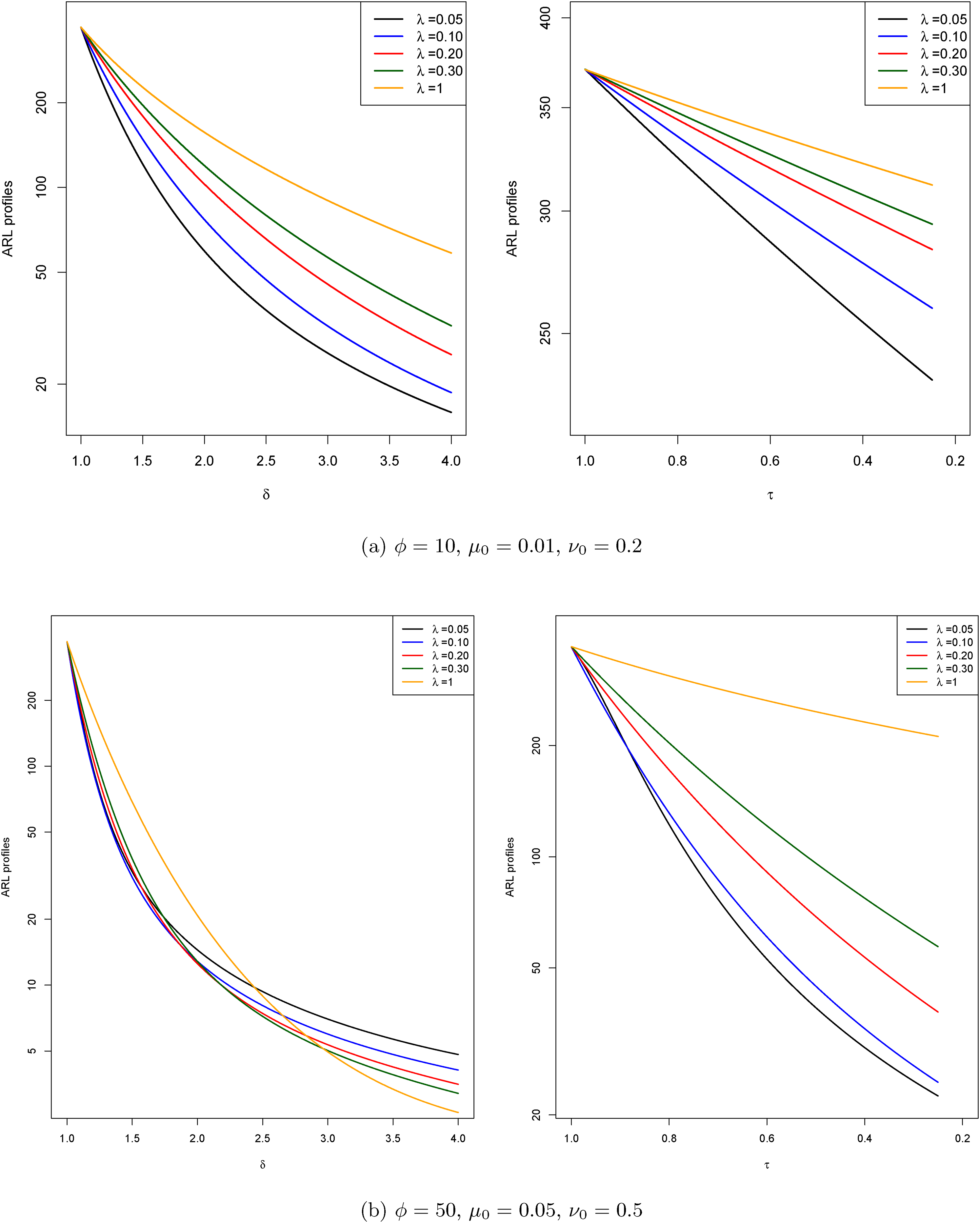
ARL comparison between BEZI-Shewhart and EWMA charts, cases 1 and 2: (a) $ϕ = 10$ , $μ_{0} = 0.01$ and $ν_{0} = 0.2$ , (b) $ϕ = 50$ , $μ_{0} = 0.05$ and $ν_{0} = 0.5$ . ARL: average run length; BEZI: zero-inflated Beta; EWMA: exponentially weighed moving average.

Figure 2.

ARL comparison between BEZI-Shewhart and EWMA charts, cases 3 and 4: (a) $ϕ = 100$ , $μ_{0} = 0.05$ and $ν_{0} = 0.2$ , (b) $ϕ = 400$ , $μ_{0} = 0.10$ and $ν_{0} = 0.8$ . ARL: average run length; BEZI: zero-inflated Beta; EWMA: exponentially weighed moving average.

Figure 3.

ARL comparison between BEZI-Shewhart and EWMA charts, cases 5 and 6: (a) $ϕ = 5$ , $μ_{0} = 0.10$ and $ν_{0} = 0.5$ , (b) $ϕ = 50$ , $μ_{0} = 0.01$ and $ν_{0} = 0.2$ . ARL: average run length; BEZI: zero-inflated Beta; EWMA: exponentially weighed moving average.

Figure 4.

ARL comparison between BEZI-Shewhart and EWMA charts, cases 7 and 8: (a) $ϕ = 100$ , $μ_{0} = 0.1$ and $ν_{0} = 0.8$ , (b) $ϕ = 400$ , $μ_{0} = 0.05$ and $ν_{0} = 0.8$ . ARL: average run length; BEZI: zero-inflated Beta; EWMA: exponentially weighed moving average.

Table 1.

IC scenarios for BEZI processes – selected cases.

Case	$ϕ$	$μ_{0}$	$ν_{0}$	$μ_{0, W}$
1	10	0.01	0.2	0.008
2	50	0.05	0.5	0.025
3	100	0.05	0.2	0.040
4	400	0.10	0.8	0.020
5	5	0.10	0.5	0.050
6	50	0.01	0.2	0.008
7	100	0.10	0.8	0.020
8	400	0.05	0.8	0.010

IC: in-control; BEZI: zero-inflated Beta.

Figures 1 to 4 reveal that the BEZI-EWMA chart outperforms the BEZI-Shewhart chart in almost all the considered cases, especially in the case of shifts only in $ν_{0}$ . For shifts only in $μ_{0}$ , the BEZI-Shewhart is preferable to the BEZI-EWMA in the cases with large $ϕ$ values (e.g. $ϕ = 100$ or 400). The ARL profiles in cases 1, 5 and 6 reveal that the BEZI-EWMA chart with $λ = 0.05$ is the best chart in detecting shifts either only in $μ_{0}$ or only in $ν_{0}$ . Similar results are given for case 2 but, for very small decreasing shifts in $ν_{0}$ (i.e. $τ \geq 0.8$ ), the BEZI-EWMA chart with $λ = 0.10$ has the best performance. The results from case 3 suggest using $λ = 0.30$ for decreasing shifts $τ \geq 0.8$ in $ν_{0}$ . For shifts only in $μ_{0}$ , the BEZI-EWMA charts with $λ \in {0.05, 0.10, 0.20, 0.30}$ have comparable and similar performance to each other, better than the ARL performance of the BEZI-Shewhart chart, for shifts $δ \leq 2$ . Finally, the results for cases 4, 7 and 8 show that the BEZI-EWMA chart with $λ = 0.05$ is the best chart for shifts $τ \leq 0.60$ in $ν_{0}$ while, for shifts only in $μ_{0}$ , the BEZI-Shewhart chart outperforms the BEZI-EWMA chart, even for $δ \leq 2.5$ .

In addition, the results of our numerical analysis reveal that there are several cases, especially for small $ϕ$ values, with $ν_{0} = 0.2$ or $0.5$ (cases of small to moderate excess of zero values), and for small shifts (e.g. $δ \leq 1.2$ or $τ \geq 0.7$ ), where the respective ${ARL}_{1}$ values are $> 200$ or even $300$ . See, for example, cases 1, 3 and 6. Compared to the IC value ${ARL}_{0} \approx 370.4$ , we deduce from the ${ARL}_{1}$ value that the chart is not able to detect quickly this type of change in the process mean level. Therefore, in this case, we suggest practitioners to evaluate the performance of the control chart by also taking into account the values of other RL-based metrics, such as the MRL or the 0.95-percentile point ${RL}_{0.95}$ .

Concerning the performance of the proposed charts under the SDRL (see Figures 1–4 in Supplemental material), the BEZI-EWMA chart with $λ = 0.05$ has the minimum SDRL for almost all shifts in $μ_{0}$ or in $ν_{0}$ . This is the case in cases 1, 5 and 6. A small SDRL value shows a stable performance for a chart. Also, the results in cases 4, 7 and 8 show that for shifts only in $μ_{0}$ , the minimum SDRL is attained by the BEZI-Shewhart chart, for almost all the shifts $δ$ while, for shifts only in $ν_{0}$ , the minimum SDRL is attained by the BEZI-EWMA chart. Finally, in case 2, we notice that the BEZI-EWMA chart with $λ = 0.05$ is the one with the smaller SDRL values, for shifts $δ \leq 2.5$ in $μ_{0}$ while for shifts only in $ν_{0}$ , the BEZI-EWMA with $λ = 0.10$ attains the minimum SDRL for shifts $τ \geq 0.8$ . Finally, the results for case 3 show that for shifts only in $μ_{0}$ , the SDRL for all the considered BEZI-EWMA charts are similar and comparable to each other, whereas, for shifts only in $ν_{0}$ , the BEZI-EWMA chart with $λ = 0.05$ attains the minimum SDRL value for $τ < 0.8$ . Similar conclusions can be drawn for the performance of the charts in terms of MRL and ${RL}_{0.95}$ . See Figures 5 to 12 in Supplemental material.

By taking into account the results of our numerical analysis, we suggest the use of the BEZI-EWMA chart with $λ = 0.05$ or 0.10, especially for small $ϕ$ values (e.g. $ϕ < 50$ ). When we are interested in detecting shifts only in $ν_{0}$ , this is also valid for larger $ϕ$ values. For larger $ϕ$ values, the BEZI-EWMA chart with larger $λ$ values, such as 0.30 or 0.20, has better performance than a BEZI-EWMA chart with $λ = 0.05$ or 0.10. However, as our analysis showed, in these cases, the BEZI-Shewhart chart has better performance, even for small shifts in $μ_{0}$ . Since the BEZI-Shewhart chart is much simpler in implementation and interpretation than the BEZI-EWMA chart, we suggest its use in these cases.

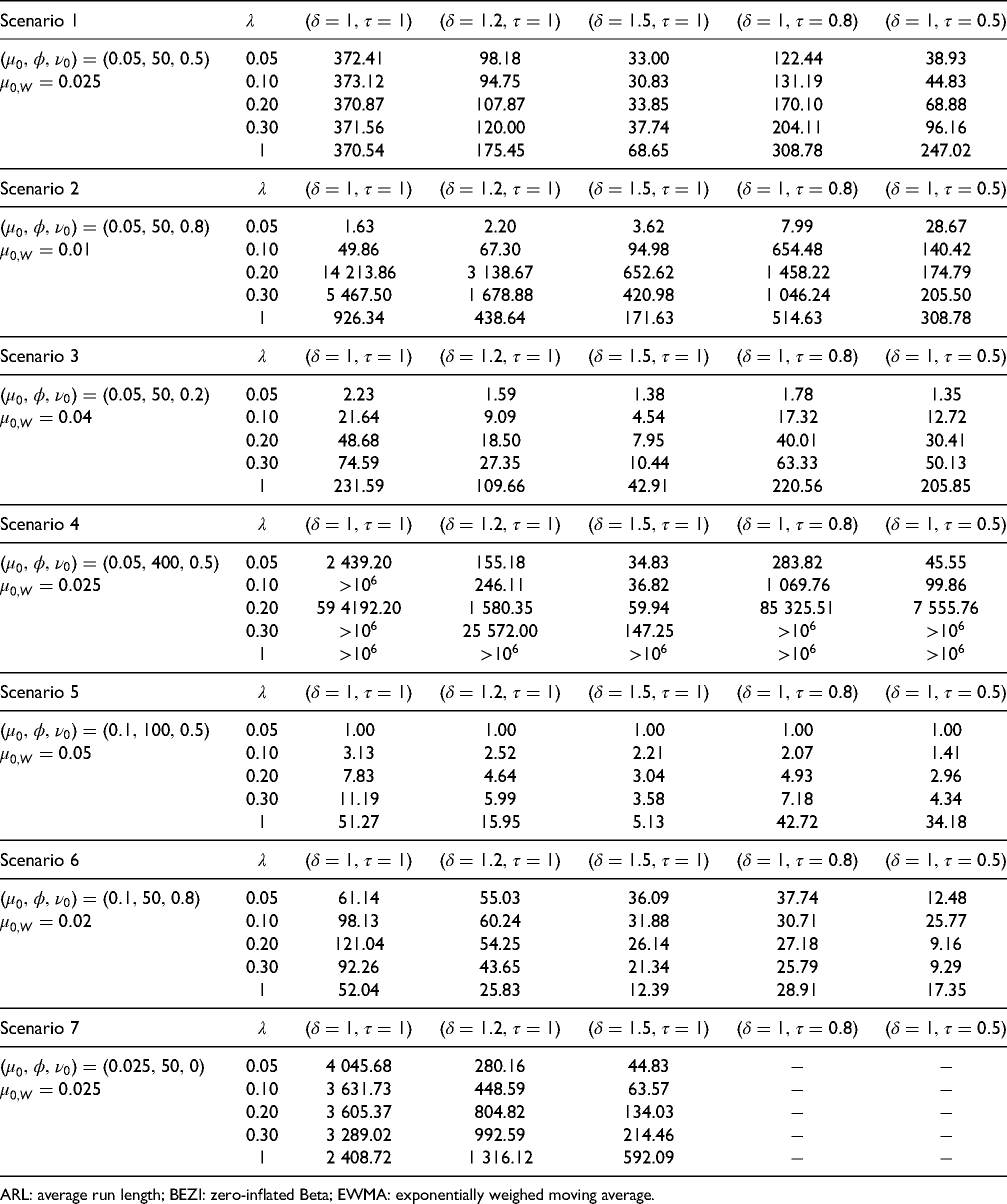
In order to analyse further the sensitivity of the considered charts against various OOC scenarios, we conducted also a simulation study. Specifically, we considered as a baseline model the case $μ_{0} = 0.05$ , $ν_{0} = 0.5$ , $ϕ = 50$ and five different charts: The upper one-sided BEZI-Shewhart chart with $UCL = 0.15779$ as well as the BEZI-EWMA chart with $(λ, L) \in {(0.05, 2.476), (0.10, 2.759), (0.20, 3.166), (0.30, 3.412)}$ . The corresponding limits are $(LCL, UCL) \in {(0.01191, 0.03809)$ , $(0.00410, 0.04590)$ , $(- 0.00985, 0.05985)$ , $(- 0.02234, 0.07234)}$ . For the charts with $LCL < 0$ , only an upper control limit is used and the LCL is set equal to 0. Also, the lines in Table 2 with $λ = 0.05$ , 0.10, 0.20, and 0.30 refer to the respective BEZI-EWMA charts while the line $λ = 1$ refers to the upper one-sided BEZI-Shewhart chart.

Table 2.

ARL values for the BEZI-EWMA chart with $λ \in {0.05, 0.10, 0.20, 0.30}$ and BEZI-Shewhart charts ( $λ = 1.00$ ) for various shifts in $μ_{0}$ or in $ν_{0}$ and for seven different BEZI processes.

Scenario 1	$λ$	$(δ = 1, τ = 1)$	$(δ = 1.2, τ = 1)$	$(δ = 1.5, τ = 1)$	$(δ = 1, τ = 0.8)$	$(δ = 1, τ = 0.5)$
$(μ_{0}, ϕ, ν_{0}) = (0.05, 50, 0.5)$	0.05	372.41	98.18	33.00	122.44	38.93
$μ_{0, W} = 0.025$	0.10	373.12	94.75	30.83	131.19	44.83
	0.20	370.87	107.87	33.85	170.10	68.88
	0.30	371.56	120.00	37.74	204.11	96.16
	1	370.54	175.45	68.65	308.78	247.02
Scenario 2	$λ$	$(δ = 1, τ = 1)$	$(δ = 1.2, τ = 1)$	$(δ = 1.5, τ = 1)$	$(δ = 1, τ = 0.8)$	$(δ = 1, τ = 0.5)$
$(μ_{0}, ϕ, ν_{0}) = (0.05, 50, 0.8)$	0.05	1.63	2.20	3.62	7.99	28.67
$μ_{0, W} = 0.01$	0.10	49.86	67.30	94.98	654.48	140.42
	0.20	14 213.86	3 138.67	652.62	1 458.22	174.79
	0.30	5 467.50	1 678.88	420.98	1 046.24	205.50
	1	926.34	438.64	171.63	514.63	308.78
Scenario 3	$λ$	$(δ = 1, τ = 1)$	$(δ = 1.2, τ = 1)$	$(δ = 1.5, τ = 1)$	$(δ = 1, τ = 0.8)$	$(δ = 1, τ = 0.5)$
$(μ_{0}, ϕ, ν_{0}) = (0.05, 50, 0.2)$	0.05	2.23	1.59	1.38	1.78	1.35
$μ_{0, W} = 0.04$	0.10	21.64	9.09	4.54	17.32	12.72
	0.20	48.68	18.50	7.95	40.01	30.41
	0.30	74.59	27.35	10.44	63.33	50.13
	1	231.59	109.66	42.91	220.56	205.85
Scenario 4	$λ$	$(δ = 1, τ = 1)$	$(δ = 1.2, τ = 1)$	$(δ = 1.5, τ = 1)$	$(δ = 1, τ = 0.8)$	$(δ = 1, τ = 0.5)$
$(μ_{0}, ϕ, ν_{0}) = (0.05, 400, 0.5)$	0.05	2 439.20	155.18	34.83	283.82	45.55
$μ_{0, W} = 0.025$	0.10	$> 10^{6}$	246.11	36.82	1 069.76	99.86
	0.20	59 4192.20	1 580.35	59.94	85 325.51	7 555.76
	0.30	$> 10^{6}$	25 572.00	147.25	$> 10^{6}$	$> 10^{6}$
	1	$> 10^{6}$	$> 10^{6}$	$> 10^{6}$	$> 10^{6}$	$> 10^{6}$
Scenario 5	$λ$	$(δ = 1, τ = 1)$	$(δ = 1.2, τ = 1)$	$(δ = 1.5, τ = 1)$	$(δ = 1, τ = 0.8)$	$(δ = 1, τ = 0.5)$
$(μ_{0}, ϕ, ν_{0}) = (0.1, 100, 0.5)$	0.05	1.00	1.00	1.00	1.00	1.00
$μ_{0, W} = 0.05$	0.10	3.13	2.52	2.21	2.07	1.41
	0.20	7.83	4.64	3.04	4.93	2.96
	0.30	11.19	5.99	3.58	7.18	4.34
	1	51.27	15.95	5.13	42.72	34.18
Scenario 6	$λ$	$(δ = 1, τ = 1)$	$(δ = 1.2, τ = 1)$	$(δ = 1.5, τ = 1)$	$(δ = 1, τ = 0.8)$	$(δ = 1, τ = 0.5)$
$(μ_{0}, ϕ, ν_{0}) = (0.1, 50, 0.8)$	0.05	61.14	55.03	36.09	37.74	12.48
$μ_{0, W} = 0.02$	0.10	98.13	60.24	31.88	30.71	25.77
	0.20	121.04	54.25	26.14	27.18	9.16
	0.30	92.26	43.65	21.34	25.79	9.29
	1	52.04	25.83	12.39	28.91	17.35
Scenario 7	$λ$	$(δ = 1, τ = 1)$	$(δ = 1.2, τ = 1)$	$(δ = 1.5, τ = 1)$	$(δ = 1, τ = 0.8)$	$(δ = 1, τ = 0.5)$
$(μ_{0}, ϕ, ν_{0}) = (0.025, 50, 0)$	0.05	4 045.68	280.16	44.83	$-$	$-$
$μ_{0, W} = 0.025$	0.10	3 631.73	448.59	63.57	$-$	$-$
	0.20	3 605.37	804.82	134.03	$-$	$-$
	0.30	3 289.02	992.59	214.46	$-$	$-$
	1	2 408.72	1 316.12	592.09	$-$	$-$

ARL: average run length; BEZI: zero-inflated Beta; EWMA: exponentially weighed moving average.

Then, we simulated seven different BEZI processes, which are as follows:

Scenario 1: $(μ_{0}, ϕ, ν_{0}) = (0.05, 50, 0.5)$ and $μ_{0, W} = 0.025$ , that is, the baseline or true model.

Scenario 2: $(μ_{0}, ϕ, ν_{0}) = (0.05, 50, 0.8)$ and $μ_{0, W} = 0.01$ , that is the probability of zero-occurrence has been increased and the process mean level has been decreased.

Scenario 3: $(μ_{0}, ϕ, ν_{0}) = (0.05, 50, 0.2)$ and $μ_{0, W} = 0.04$ , that is, the probability of zero-occurrence has been decreased and the process mean level has been increased.

Scenario 4: $(μ_{0}, ϕ, ν_{0}) = (0.05, 400, 0.5)$ and $μ_{0, W} = 0.025$ , that is, parameter $ϕ$ has been increased but the process mean level remains the same.

Scenario 5: $(μ_{0}, ϕ, ν_{0}) = (0.1, 100, 0.5)$ and $μ_{0, W} = 0.05$ , that is, parameters $ϕ$ and $μ_{0}$ have been increased and the process mean level has been increased as well.

Scenario 6: $(μ_{0}, ϕ, ν_{0}) = (0.1, 50, 0.8)$ and $μ_{0, W} = 0.02$ , that is, parameters $μ_{0}$ and $ν_{0}$ have been increased and the process mean level has been decreased.

Scenario 7: $(μ_{0}, ϕ, ν_{0}) = (0.025, 50, 0.0)$ and $μ_{0, W} = 0.025$ , that is parameter $μ_{0}$ has been decreased, $ν_{0} = 0$ (case of Beta distribution) and the process mean level equals the one of the IC model.

For each scenario, we simulated 100,000 BEZI processes and applied the five charts that have been developed under the baseline model introduced above. Then, we estimated (from the 100,000 run-length values) the ARL for various shifts in process parameters. These values are given in the entries of Table 2. The standard error of the estimation, that is,

S D R L / \sqrt{10^{5}}

, is below 1.

Then, we modified the IC parameter values (scenarios 2 to 7) and applied again the five charts in order to assess the robustness of the proposed charts on deviations from the IC model. The results from the simulation study reveal that if the parameter $ν_{0}$ is actually larger or smaller than expected, then the BEZI-EWMA chart either has an increased FAR (cases $λ = 0.05$ and 0.10 in Scenarios 2 and 3) or it is very small, with very large IC $A R L$ values (cases $λ = 0.20$ and 0.30 in Scenarios 2 and 3). Note also that if $ϕ$ value is actually much larger than expected (Scenario 4), then the IC ARL value becomes very large and the BEZI-EWMA chart is not very sensitive in the detection of small shifts in $μ_{0}$ or in $ν_{0}$ , especially for $λ \geq 0.20$ . However, for $λ = 0.05$ or 0.10, the BEZI-EWMA, even, in this case, has a good ability to detect small shifts only in $μ_{0}$ .

When only $ν_{0}$ does not change (case of Scenario 5), the chart has an increased FAR. In this scenario, the actual IC process mean $μ_{0, W}$ is twice the IC mean of the baseline model in Scenario 1 and the BEZI-EWMA chart signals almost immediately. In Scenario 6, both $μ_{0}$ and $ν_{0}$ are larger than expected, resulting in an IC mean slightly smaller than the IC mean in Scenario 1. However, the BEZI-EWMA chart has an increased FAR, especially for small or large $λ$ values.

In the last scenario, it is not possible to observe zero values in the data and even the IC mean equals the IC mean in Scenario 1, the BEZI-EWMA charts have an increased IC ARL value, which also affects their ability in the detection of small shifts in $μ_{0}$ . Only for large increasing shifts in $μ_{0}$ , the OOC ARL values are comparable to that obtained under the baseline model and only for $λ = 0.05$ . Also, in this scenario $ν_{0} = 0$ and for $τ = 0.8$ or 0.5, $ν_{1} = τ ν_{0} = 0$ , that is, no changes occur to $ν_{0}$ and the respective entries are marked with ‘ $-$ ’.

Similar conclusions are also derived for the robustness of the BEZI-Shewhart chart, when the actual IC values of the process parameters have not been determined properly. In Scenario 4, the BEZI-Shewhart chart cannot detect any of the shifts in the values of the process parameters. In Scenario 2, the IC ARL value is approximately three times the desired one and this has also an effect on its OOC performance; the respective OOC ARL values are much larger, compared to the ones for the baseline model. For the remaining scenarios (3, 5 and 6), the BEZI-Shewhart chart has an increased FAR (equivalently, the IC ARL is lower than the desired value). When the true model is that of the Beta distribution (Scenario 7), the IC performance of the BEZI-Shewhart is similar to that of the BEZI-EWMA chart. However, its OOC performance is much more affected, even for large shifts to $μ_{0}$ . Due to the presence of zero values, the BEZI model is over-dispersed, compared to the Beta model. The variance of the $BEZI (0.05, 50, 0.5)$ distribution equals 0.001 091, whereas the variance for the Beta distribution with $μ_{0} = 0.025$ and $ϕ = 50$ equals 0.000 478. We attribute the difference in the ARL values of the proposed charts to the difference between the variances of the $BEZI (0.05, 50, 0.5)$ (Scenario 1) and $BEZI (0.025, 50, 0)$ (Scenario 7) models.

5 An illustrative example

In the literature of statistical modelling, the BEZI distribution has been applied (among others) for the statistical modelling of the percentage of qualified nurses in Brazilian municipalities,²⁸ the proportions of deaths caused by traffic accidents,⁴¹ the reading skills of children in primary schools,^43,42 the proportion of rapid eye movement sleep time,⁴⁴ the diet composition in fatty acid signature analysis⁴⁵ and in word frequency analysis.⁴⁶

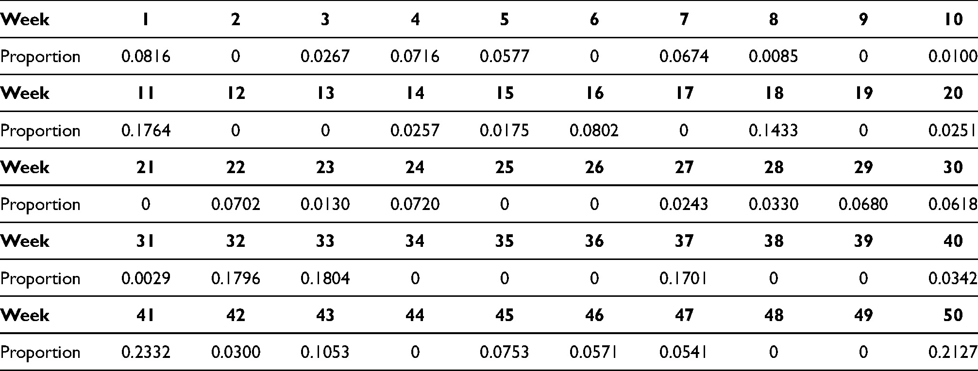
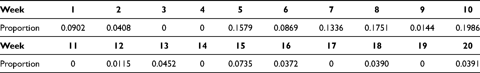
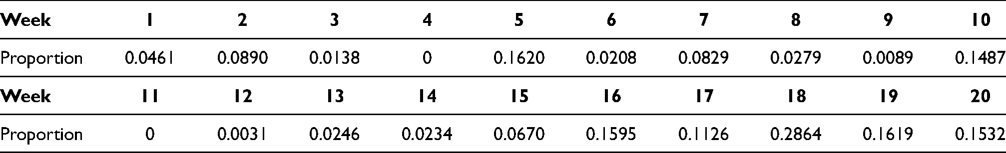
In this section, we demonstrate the practical implementation of the BEZI-Shewhart and BEZI-EWMA charts with simulated data. Ospina and Ferrari⁴¹ illustrated the utility of the BEZI distribution in analysing the mortality due to traffic accidents in 200 Brazilian municipalities in 2002. The results from their analysis revealed that 39% of reported deaths were not caused by traffic accidents, while the expected proportion of deaths is 0.05 with a standard deviation equal to 0.07. Based on these findings, we consider the following simulated data (see Tables 3–5), which refer to, say, the weekly proportions of deaths caused by traffic accidents. The baseline model is the $BEZI (0.08, 15, 0.4),$ which is very close to the one estimated by Ospina and Ferrari.⁴¹ Specifically, we assume a probability $ν_{0} = 0.4$ for a death that was not caused by a traffic accident while the expected weekly proportion of deaths caused by traffic accidents equals 0.048, by applying equation (7) for $ν = 0.4$ and $μ = 0.08$ . This is the IC process mean level $μ_{0, W}$ . Also, for $ν = 0.4$ , $μ = 0.08$ , $ϕ = 15$ and by applying equation (7), we deduce that the IC variance of the BEZI process equals 0.00430. Therefore, both IC mean and variance are very close to the values 0.05 and $0.0049 = {0.07}^{2}$ , estimated by Ospina and Ferrari.⁴¹ The values in Table 3 have been simulated from a $BEZI (0.08, 15, 0.4)$ distribution and they represent the IC period. Also, we simulated two different OOC scenarios. In the first (Table 4), there is an increase in the proportion of deaths due to an increase in $μ_{0}$ while in the second, the increase in proportion is due to a decrease in $ν_{0}$ (Table 5). All the available data are given with four decimals accuracy.

Table 3.
Proportion of weekly deaths caused by traffic accidents, in-control (IC) data.

Week 1 2 3 4 5 6 7 8 9 10

Proportion 0.0816 0 0.0267 0.0716 0.0577 0 0.0674 0.0085 0 0.0100

Week 11 12 13 14 15 16 17 18 19 20

Proportion 0.1764 0 0 0.0257 0.0175 0.0802 0 0.1433 0 0.0251

Week 21 22 23 24 25 26 27 28 29 30

Proportion 0 0.0702 0.0130 0.0720 0 0 0.0243 0.0330 0.0680 0.0618

Week 31 32 33 34 35 36 37 38 39 40

Proportion 0.0029 0.1796 0.1804 0 0 0 0.1701 0 0 0.0342

Week 41 42 43 44 45 46 47 48 49 50

Proportion 0.2332 0.0300 0.1053 0 0.0753 0.0571 0.0541 0 0 0.2127

Week	1	2	3	4	5	6	7	8	9	10
Proportion	0.0816	0	0.0267	0.0716	0.0577	0	0.0674	0.0085	0	0.0100
Week	11	12	13	14	15	16	17	18	19	20
Proportion	0.1764	0	0	0.0257	0.0175	0.0802	0	0.1433	0	0.0251
Week	21	22	23	24	25	26	27	28	29	30
Proportion	0	0.0702	0.0130	0.0720	0	0	0.0243	0.0330	0.0680	0.0618
Week	31	32	33	34	35	36	37	38	39	40
Proportion	0.0029	0.1796	0.1804	0	0	0	0.1701	0	0	0.0342
Week	41	42	43	44	45	46	47	48	49	50
Proportion	0.2332	0.0300	0.1053	0	0.0753	0.0571	0.0541	0	0	0.2127

Table 4.

Proportion of weekly deaths caused by traffic accidents, out-of-control process (OOC) data, increase in $μ_{0}$ .

Week	1	2	3	4	5	6	7	8	9	10
Proportion	0.0902	0.0408	0	0	0.1579	0.0869	0.1336	0.1751	0.0144	0.1986
Week	11	12	13	14	15	16	17	18	19	20
Proportion	0	0.0115	0.0452	0	0.0735	0.0372	0	0.0390	0	0.0391

Table 5.

Proportion of weekly deaths caused by traffic accidents, out-of-control process (OOC) data, decrease in $ν_{0}$ .

Week	1	2	3	4	5	6	7	8	9	10
Proportion	0.0461	0.0890	0.0138	0	0.1620	0.0208	0.0829	0.0279	0.0089	0.1487
Week	11	12	13	14	15	16	17	18	19	20
Proportion	0	0.0031	0.0246	0.0234	0.0670	0.1595	0.1126	0.2864	0.1619	0.1532

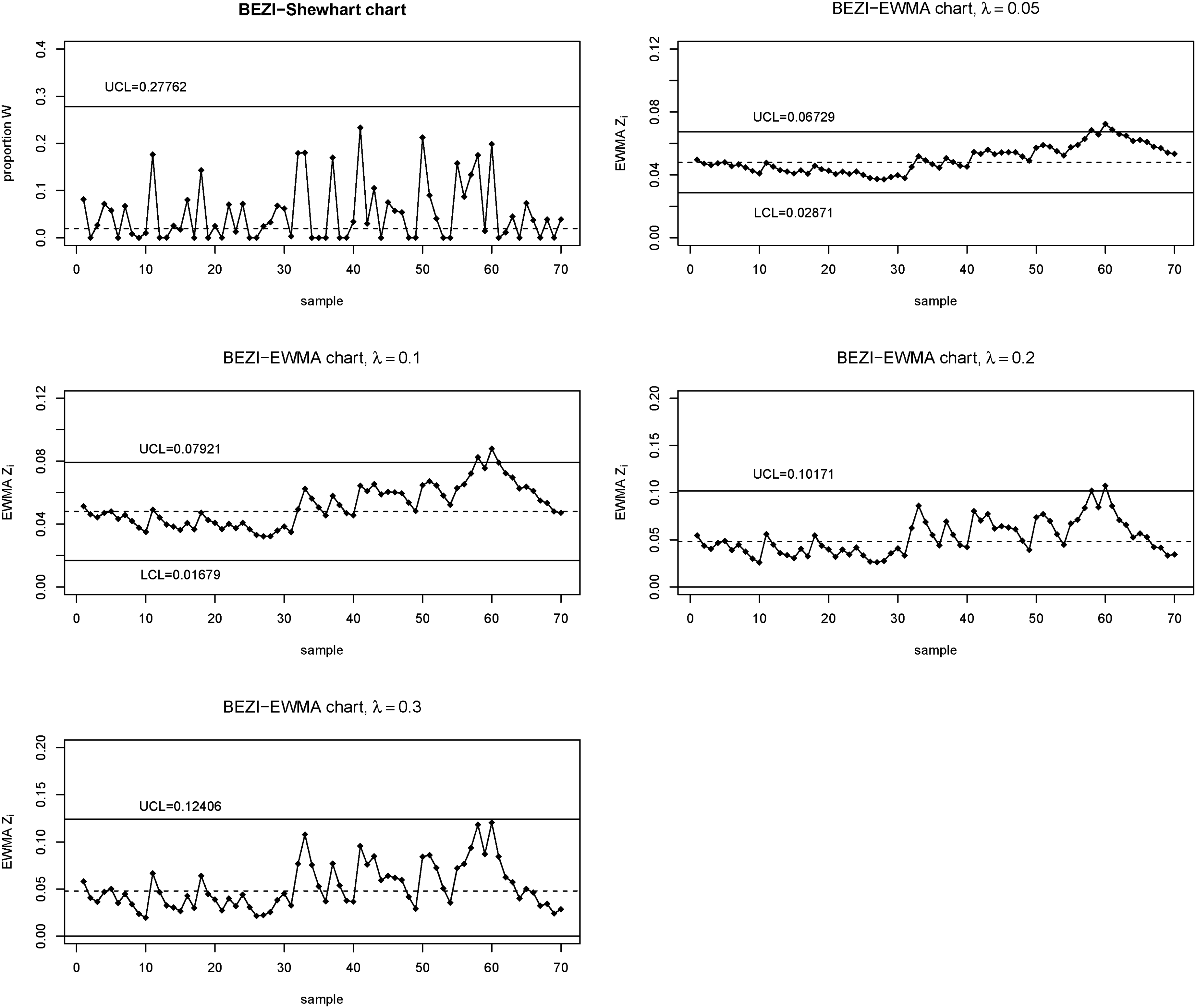
Next, we proceed with the determination of the control limits for the BEZI-Shewhart chart and the BEZI-EWMA chart. For illustrative purposes, we choose $A R L_{0} \approx 100$ . This means that even if there is not an increase in the weekly proportion of deaths caused by traffic accidents, an OOC signal will be generated every 100 points, on average. Since the data are on a weekly basis, we expect a (false) signal for an increase in the proportion of deaths within (approximately) two years (based on 52 weeks per year). The control limit for the upper one-sided BEZI-Shewhart chart is ${UCL}_{SH} = 0.27762$ .

By applying the methodology described in Section 4, we determine the value $L$ for $λ \in {0.05, 0.10, 0.20, 0.30}$ . We mention that, in practise, there are cases for which we do not know anything about the magnitude of possible (if any) shifts in the process parameters. Therefore, we apply four different BEZI-EWMA charts, with various values for $λ$ . The empirical rule is that Shewhart charts are applied for sudden shifts of large magnitude in process parameter(s) whereas EWMA charts are preferable for shifts of small magnitude. As already said at the end of the previous section, values $λ = 0.05$ or 0.10 are good in the detection of small shifts in the process parameters; for larger shifts, the BEZI-EWMA chart with $λ = 0.20$ or 0.30 has a better performance.

The values of the pairs $(λ, L)$ are ${(0.05, 1.838), (0.10, 2.076), (0.20, 2.458), (0.30, 2.762)}$ with the respective control limits equal to $(LCL, UCL) \in {(0.02871, 0.06729)$ , $(0.01679, 0.07921)$ , $(- 0.00571, 0.10171)$ and $(- 0.02806, 0.12406)}$ . We note here that when $LCL < 0$ , we set it equal to 0.

All the five charts, for each of the different OOC situations, are given in Figures 5 and 6. The dashed line represents the centre line of each chart. In the case of the BEZI-Shewhart chart, it is the median of the IC BEZI distribution while, in the case of the BEZI-EWMA chart, it is the expected value of the IC BEZI distribution. The median of IC BEZI distribution is approximately equal to 0.01962. It is not difficult to see that none of the charts gives a false alarm signal because none of the points from 1 to 50 (IC period) is beyond the control limits. The BEZI-Shewhart chart does not give an OOC signal when there is a shift in $μ_{0}$ while, except for the case $λ = 0.30$ , the BEZI-EWMA charts give an OOC signal at point 58, for the first time. This OOC situation corresponds to a (simulated) shift $δ = 1.2$ and probably, it is not of a large magnitude to be detected by the Shewhart chart.

Figure 5.

Phase II BEZI-Shewhart and BEZI-EWMA charts for the simulated data in Tables 3 and 4. BEZI: zero-inflated Beta; EWMA: exponentially weighed moving average.

Figure 6.

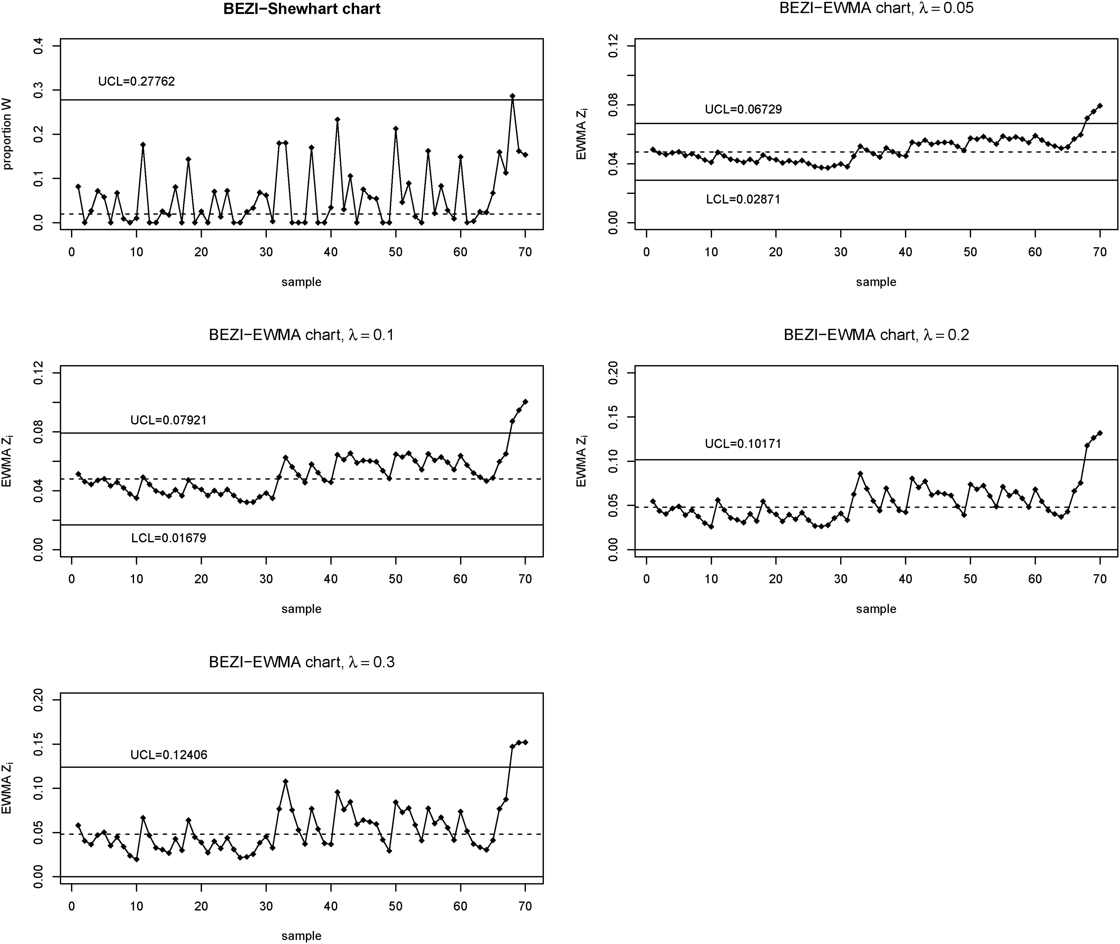
Phase II BEZI-Shewhart and BEZI-EWMA charts for the simulated data in Tables 3 and 5. BEZI: zero-inflated Beta; EWMA: exponentially weighed moving average.

When there is a shift in $ν_{0}$ , then all charts declare the process as OOC for the first time at point 68. This OOC situation corresponds to a (simulated) shift $τ = 0.5$ , which is of large magnitude. However, not only the Shewhart chart but also the EWMA charts, detect this shift.

6 Conclusions

In this work, we studied the EWMA chart in the monitoring of proportions with an excessive number of zero values. We assumed that the process is modelled according to a BEZI distribution. This setup is common in various types of processes, especially in health-related ones. The BEZI-EWMA chart was compared with the BEZI-Shewhart chart and demonstrated a significantly improved performance, in terms of several measures based on the run-length distribution. For a small IC value for the precision parameter $ϕ$ , the BEZI-EWMA chart outperforms (in terms of ${ARL}_{1}$ ) the BEZI-Shewhart chart, especially when there is a shift only in parameter $ν$ . As $ϕ$ increases (and the other IC parameter values $μ_{0}$ , $ν_{0}$ remain the same), the reduction achieved in the ${ARL}_{1}$ values can be up to 45%, for shifts $δ = 1.2$ or $τ = 0.8$ . However, for very large $ϕ$ values, the picture is reversed and the BEZI-Shewhart chart has better performance than the BEZI-EWMA chart, especially in the detection of shifts only in $μ_{0}$ parameter. For BEZI processes with a high probability of zero values, the performance of both charts is affected, as well. As a general guideline for practitioners, we suggest the use of a BEZI-EWMA chart with $λ = 0.05$ or 0.10, for the detection of shifts only in $μ_{0}$ or only in $ν_{0}$ . For large $ϕ$ values (e.g. $ϕ \geq 100$ ), we suggest either the use of the BEZI-EWMA chart with $λ = 0.20$ or 0.30 or even the BEZI-Shewhart chart, especially when we want to detect changes only in $μ_{0}$ and the value $ν_{0} > 0.5$ .

A simulation study was conducted in order to assess the robustness and the sensitivity of the proposed charts when the true IC model differs from the assumed one. The results showed that even small deviations from the true IC model have a significant effect on the performance of the chart, especially in the case where the true $ϕ$ value is larger than expected or when at least one of the process parameters have not been determined correctly. Therefore, the (true) IC values of the process parameters need to be determined carefully. For this purpose, a detailed Phase I analysis needs to be conducted first. Moreover, since in practise the process parameters are rarely known and before applying the control chart they have to be estimated, a separate study is necessary on the effect of estimated parameters on the chart’s performance. For all these topics, research is undergoing and the results will be presented in a future paper.

A limitation of the present study is that we consider shifts in exactly one of the parameters $μ$ or $ν$ of the process. We believe that the case of simultaneous shifts in process parameters has to be treated with at least two control charts, one for each parameter. It is important not only to detect the change but also to identify (if possible) which of the parameters have changed. Under this framework, the detection of changes in $ϕ$ can be also studied. However, multiple schemes have to be designed and applied simultaneously. A useful technique in that direction is the CUSUM chart based on the likelihood ratio statistic.

Finally, the R codes for verifying the results presented in this paper are available at https://github.com/arakitz/BEZIcharts

Supplemental Material

sj-pdf-1-smm-10.1177_09622802221074157 - Supplemental material for Exponentially weighed moving average charts for monitoring zero-inflated proportions with applications in health care

Supplemental material, sj-pdf-1-smm-10.1177_09622802221074157 for Exponentially weighed moving average charts for monitoring zero-inflated proportions with applications in health care by Petros E. Maravelakis, Athanasios C. Rakitzis and Philippe Castagliola in Statistical Methods in Medical Research

Footnotes

Acknowledgements

The authors would like to express their gratitude to the two anonymous reviewers for their constructive comments, which improved significantly the content and the presentation of this paper.

Declaration of conflicting interests

The authors declared no potential conflicts of interest with respect to the research, authorship and/or publication of this article.

Funding

The authors received no financial support for the research, authorship and/or publication of this article.

ORCID iD

Petros E. Maravelakis

Supplemental material

Supplementary material for this article is available online.

Appendix 1

In this Appendix, we provide the details of the Markov chain technique that was employed for the study of the BEZI-EWMA chart. Let us consider (in general) a two-sided BEZI-EWMA chart with control limits LCL, UCL and $LCL < UCL$ . In order to apply the Markov chain technique, we divide first the interval $[LCL, UCL]$ into $2 m + 1$ subintervals $(H_{j} - Δ, H_{j} + Δ]$ , $j \in {1, \dots, m + 1, \dots, 2 m + 1}$ , centred at

H_{j} = \frac{LCL + UCL}{2} + 2 j Δ

where

2 Δ = (UCL - LCL) / (2 m + 1)

. The transient states of the Markov chain are represented using the subinterval

(H_{j} - Δ, H_{j} + Δ]

. If

Z_{i} \in (H_{j} - Δ, H_{j} + Δ]

then we deduce that at sample

i

, the Markov chain is in the transient state

j

for sample

i

. Moreover, if for every

j \in {1, 2, \dots, 2 m + 1}

the

Z_{i} \notin (H_{j} - Δ, H_{j} + Δ]

then we deduce that the Markov chain has reached the absorbing state

(- \infty, LCL] \cup [UCL, + \infty)

. Clearly, when the Markov chain reaches the absorbing state, the BEZI-EWMA chart gives an OOC signal. Also, we assume that

H_{j}

is the representative value of state

j \in {1, \dots, m + 1, \dots, 2 m + 1}

The transition probability matrix $P$ of this discrete-time Markov chain is written in the form:

P = (\begin{matrix} Q & r \\ 0^{T} & 1 \end{matrix})

where

Q

is the

(2 m + 1, 2 m + 1)

matrix of transient probabilities

q_{i, j}

r = 1 - Q 1

(i.e. row probabilities sum to 1),

0^{T} = (0, 0, \dots, 0)

and

1 = (1, 1, \dots, 1)^{T} ⊺

. The form of matrix

Q

is the following: (\text A.1)

Q = (\begin{matrix} q_{1, 1} & \dots & q_{1, m} & q_{1, m + 1} & \dots & q_{1, 2 m + 1} \\ ⋮ & ⋮ & ⋮ & ⋮ & ⋮ & ⋮ \\ q_{m, 1} & \dots & q_{m, m} & q_{m, m + 1} & \dots & q_{m, 2 m + 1} \\ q_{m + 1, 1} & \dots & q_{m + 1, m} & q_{m + 1, m + 1} & \dots & q_{m + 1, 2 m + 1} \\ ⋮ & ⋮ & ⋮ & ⋮ & ⋮ & ⋮ \\ q_{2 m + 1, 1} & \dots & q_{2 m + 1, m} & q_{2 m + 1, m + 1} & \dots & q_{2 m + 1, 2 m + 1} \end{matrix})

The computation of the transition probabilities between the transient states of the Markov chain can be done by using the relation

q_{j, k} = P (Z_{i} \in (H_{k} - Δ, H_{k} + Δ] | Z_{i - 1} = H_{j}), j, k \in {1, 2, \dots, 2 m + 1}

or equivalently

q_{j, k} = P (Z_{i} \leq H_{k} + Δ | Z_{i - 1} = H_{j}) - P (Z_{i} \leq H_{k} - Δ | Z_{i - 1} = H_{j})

Given that

Z_{i - 1} = H_{j}

and by using (9), we derive (after isolating

W_{i}

) the following expression for

q_{i j}

\begin{aligned} q_{j, k} & = P (W_{i} \leq \frac{H_{k} + Δ - (1 - λ) H_{j}}{λ}) - P (W_{i} \leq \frac{H_{k} - Δ - (1 - λ) H_{j}}{λ}) \\ = F_{BEZI} (\frac{H_{k} + Δ - (1 - λ) H_{j}}{λ} | μ, ϕ, ν) - F_{BEZI} (\frac{H_{k} - Δ - (1 - λ) H_{j}}{λ} | μ, ϕ, ν) \end{aligned}

Let also

q = (q_{1}, \dots, q_{m + 1}, \dots, q_{2 m + 1})^{⊺}

be the

(2 m + 1, 1)

vector of initial probabilities associated with the

2 m + 1

transient states of the Markov chain. Then, for

j \in {1, 2, \dots, 2 m + 1}

(\text A.2)

q_{j} = {\begin{matrix} 0 & if Z_{0} \notin (H_{j} - Δ, H_{j} + Δ] \\ 1 & if Z_{0} \in (H_{j} - Δ, H_{j} + Δ] \end{matrix}

Provided that the number

2 m + 1

of subintervals in matrix

Q

is sufficiently large (e.g. we may set

m = 200

, i.e.

2 m + 1 = 401

), we accurately evaluate the RL properties of the EWMA control chart for monitoring the fraction nonconforming. In this work, we used

m = 200

in the numerical computations. The RL distribution of the EWMA control chart for monitoring the fraction nonconforming is a discrete phase-type rv with parameters

(Q, q)

.^49,48,47 The pdf

f_{RL} (ℓ)

and the cdf

F_{RL} (ℓ)

of RL are, respectively, equal to (\text A.3)

f_{RL} (ℓ) = q^{T} Q^{ℓ - 1} r

(\text A.4)

F_{RL} (ℓ) = 1 - q^{⊺} Q^{ℓ} 1

while with

1 = (1, 1, \dots, 1)^{T}

, the mean (ARL), the second non-central moment

E 2 RL = E ({RL}^{2})

and the standard deviation of RL (SDRL) are, respectively, equal to (\text A.5)

ARL = ν_{1}

(\text A.6)

E 2 RL = ν_{1} + ν_{2}

(\text A.7)

SDRL = \sqrt{E 2 RL - {ARL}^{2}}

Note also that

ν_{1}

and

ν_{2}

are the first and second factorial moments of the RL, that is (\text A.8)

ν_{1} = q^{T} (I - Q)^{- 1} 1

(\text A.9)

ν_{2} = 2 q^{T} (I - Q)^{- 2} Q 1

We mention that, in general, the form of the ARL function is quite complicated. From the previous formulas, we deduce that its determination requires matrix inversion and multiplication. Therefore, analytical formulas are not provided.

References

Bersimis

Sgora

Psarakis

. The application of multivariate statistical process monitoring in non-industrial processes. Qual Technol Quant Manage 2018; 15: 526–549.

Woodall

. The use of control charts in health-care and public-health surveillance. J Qual Technol 2006; 38: 89–104.

Woodall

Zhao

Paynabar

, et al. An overview and perspective on social network monitoring. IISE Trans 2017; 49: 354–365.

Montgomery

. Statistical quality control: A modern introduction. 7th ed. New York: Wiley, 2013.

Alencar

Lee Ho

Albarracin

OYE

. CUSUM control charts to monitor series of negative binomial count data. Stat Methods Med Res 2017; 26: 1925–1935.

Rakitzis

Castagliola

Maravelakis

. Cumulative sum control charts for monitoring geometrically inflated poisson processes: An application to infectious disease counts data. Stat Methods Med Res 2018; 27: 622–641.

Rogerson

Yamada

. Statistical detection and surveillance of geographic clusters. Boca Raton, FL: CRC Press, 2008.

Rossi

Lampugnani

Marchi

. An approximate CUSUM procedure for surveillance of health events. Stat Med 1999; 18: 2111–2122.

Sparks

Keighley

Muscatello

. Early warning CUSUM plans for surveillance of negative binomial daily disease counts. J Appl Stat 2010; 37: 1911–1929.

10.

Sparks

Keighley

Muscatello

. Optimal exponentially weighted moving average (EWMA) plans for detecting seasonal epidemics when faced with non-homogeneous negative binomial counts. J Appl Stat 2011; 38: 2165–2181.

11.

Fernandes

Bourguignon

. Control charts to monitor rates and proportions. Qual Reliab Eng Int 2019; 35: 74–83.

12.

Ali

Pievatolo

Göb

. An overview of control charts for high-quality processes. Qual Reliab Eng Int 2016; 32: 2171–2189.

13.

Aytaçoğlu

Woodall

. Dynamic probability control limits for CUSUM charts for monitoring proportions with time-varying sample sizes. Qual Reliab Eng Int 2020; 36: 592–603.

14.

Daryabari

Malmir

Amiri

. Monitoring Bernoulli processes considering measurement errors and learning effect. Qual Reliab Eng Int 2019; 35: 1129–1143.

15.

Joner Jr

Woodall

Reynolds Jr

. Detecting a rate increase using a Bernoulli scan statistic. Stat Med 2008; 27: 2555–2575.

16.

Neuburger

Walker

Sherlaw-Johnson

, et al. Comparison of control charts for monitoring clinical performance using binary data. BMJ Qual Saf 2017; 26: 919–928.

17.

Reynolds

Stoumbos

. A CUSUM chart for monitoring a proportion when inspecting continuously. J Qual Technol 1999; 31: 87–108.

18.

Rossi

Sarto

Marchi

. A new risk-adjusted Bernoulli cumulative sum chart for monitoring binary health data. Stat Methods Med Res 2016; 25: 2704–2713.

19.

Sego

Woodall

Reynolds Jr

. A comparison of surveillance methods for small incidence rates. Stat Med 2008; 27: 1225–1247.

20.

Spliid

. An exponentially weighted moving average control chart for Bernoulli data. Qual Reliab Eng Int 2010; 26: 97–113.

21.

Weiß

Atzmüller

. EWMA control charts for monitoring binary processes with applications to medical diagnosis data. Qual Reliab Eng Int 2010; 26: 795–805.

22.

Szarka

Woodall

. A review and perspective on surveillance of Bernoulli processes. Qual Reliab Eng Int 2011; 27: 735–752.

23.

Kieschnick

McCullough

. Regression analysis of variates observed on

(0, 1) :

percentages, proportions and fractions. Stat Model 2003; 3: 193–213.

24.

Bury

. Statistical distributions in engineering. New York: Cambridge University Press, 1999.

25.

Gupta

Nadarajah

. Handbook of beta distribution and its applications. New York: Marcel Dekker, 2004.

26.

Sant'Anna

ÂMO

ten Caten

. Beta control charts for monitoring fraction data. Expert Syst Appl 2012; 39: 10236–10243.

27.

de Araujo Lima-Filho

Pereira

de Souza

, et al. Inflated beta control chart for monitoring double bounded processes. Comput Ind Eng 2019; 136: 265–276.

28.

Ospina

Ferrari

SLP

. Inflated beta distributions. Stat Papers 2010; 51: 111–126.

29.

Mahmood

Xie

. Models and monitoring of zero-inflated processes: The past and current trends. Qual Reliab Eng Int 2019; 35: 2540–2557.

30.

Chen

, et al. Early dengue outbreak detection modeling based on dengue incidences in Singapore during 2012 to 2017. Stat Med 2020; 39: 2101–2114.

31.

Ferrari

Cribari-Neto

. Beta regression for modelling rates and proportions. J Appl Stat 2004; 7: 799–815.

32.

R Core Team. R: A Language and Environment for Statistical Computing. Vienna, Austria: R Foundation for Statistical Computing, 2021. https://www.R-project.org/

33.

Rigby

Stasinopoulos

. Generalized additive models for location, scale and shape, (with discussion). Appl Stat 2005; 54: 507–554.

34.

Roberts

. Control chart tests based on geometric moving averages. Technometrics 1959; 1: 239–250.

35.

Human

Kritzinger

Chakraborti

. Robustness of the EWMA control chart for individual observations. J Appl Stat 2011; 38: 2071–2087.

36.

Sparks

. Linking EWMA p charts and the risk adjustment control charts. Qual Reliab Eng Int 2017; 33: 617–636.

37.

Brook

Evans

. An approach to the probability distribution of CUSUM run length. Biometrika 1972; 3: 539–549.

38.

Bersimis

Koutras

Maravelakis

. A compound control chart for monitoring and controlling high quality processes. Eur J Oper Res 2014; 233: 595–603.

39.

Lou

WYW

. Distribution theory of runs and patterns and its applications. Singapore: World Scientific Publishing, 2003.

40.

Saccucci

Lucas

. Average run lengths for exponentially weighted moving average control schemes using the markov chain approach. J Qual Technol 1990; 22: 154–162.

41.

Ospina

Ferrari

SLP

. A general class of zero-or-one inflated beta regression models. Comput Stat Data Anal 2012; 56: 1609–1623.

42.

Liu

Eugenio

. A review and comparison of Bayesian and likelihood-based inferences in beta regression and zero-or-one-inflated beta regression. Stat Methods Med Res 2018; 27: 1024–1044.

43.

Smithson

Verkuilen

. A better lemon squeezer? Maximum-likelihood regression with beta-distributed dependent variables. Psychol Methods 2006; 11: 54.

44.

Ahmadi

Chung

Gibbs

, et al. The Berlin questionnaire for sleep apnea in a sleep clinic population: relationship to polysomnographic measurement of respiratory disturbance. Sleep Breath 2008; 12: 39–45.

45.

Stewart

. Zero-inflated beta distribution for modeling the proportions in quantitative fatty acid signature analysis. J Appl Stat 2013; 40: 985–992.

46.

Burch

Egbert

. Zero-inflated beta distribution applied to word frequency and lexical dispersion in corpus linguistics. J Appl Stat 2020; 47: 337–353.

47.

Q-M

. Fundamentals of matrix-analytic methods. New York: Springer, 2014.

48.

Latouche

Ramaswami

. Introduction to matrix analytic methods in stochastic modelling. Series on statistics and applied probability. , Philadelphia, PA: SIAM, 1999.

49.

Neuts

. Matrix-geometric solutions in stochastic models: An algorithmic approach. Baltimore, MD: Johns Hopkins University Press, 1981.

Supplementary Material

Please find the following supplemental material available below.

For Open Access articles published under a Creative Commons License, all supplemental material carries the same license as the article it is associated with.

For non-Open Access articles published, all supplemental material carries a non-exclusive license, and permission requests for re-use of supplemental material or any part of supplemental material shall be sent directly to the copyright owner as specified in the copyright notice associated with the article.

0.00 MB

0.42 MB