Unified approach to optimal estimation of mean and standard deviation from sample summaries

Abstract

Recently, various methods have been developed to estimate the sample mean and standard deviation when only the sample size, and other selected sample summaries are reported. In this paper, we provide a unified approach to optimal estimation that can be easily adopted when only some summary statistics are reported. We show that the proposed estimators have the lowest variance among linear unbiased estimators. We also show that in the most commonly reported cases, that is, when only a three-number or five-number summary is reported, the newly proposed estimators match the previously developed estimators. Finally, we demonstrate the performance of the estimators numerically.

Keywords

Interquartile range five-number summary range sample mean standard deviation

1 Introduction

When a study deals with a continuous outcome variable, one needs an estimate of the underlying standard deviation ( $σ$ ) of the observational error component in order to interpret the results. Similarly, when one wishes to combine data from multiple independent studies in a meta-analysis context, knowledge of the sample mean and sample standard deviation is essential in order to establish the precision of the results.¹ Unfortunately, some authors fail to report either the mean or the standard deviation or both. Especially for data that are skewed, or perceived to be skewed, authors often report the three-number summary, that is, the sample median, minimum and maximum^2,3; or the five-number summary, that is, the sample median, the first and third quartiles, and the minimum and maximum values.⁴ Rather than discarding the studies that do not report the sample mean and SD, one should try to estimate these quantities from their reported summaries. While the work on this problem can be traced back all the way to Tippett,⁵ interest in the systematic research of the estimators resurfaced in Hozo et al.⁶ and a significant body of the literature soon followed.^7–19 Typically, three scenarios are investigated, depending on the summaries being reported in an addition to a sample size:

Scenario 1:
${min, median, max}$ ,
Scenario 2:
${first quartile, median, third quartile}$ , or
Scenario 3:
${min, first quartile, median, third quartile, max}$ .
However, other summaries are also possible; for example, Bowley’s “seven-figure summary,” including the minimum, first deciles, first quartile, median, third quartile, last decile, and maximum.²⁰ In general, estimators for the sample mean and sample SD are developed separately and independently of each other. Moreover, the estimators are developed differently for each different scenario; see, for example, Shi et al.¹³

In this paper, we propose a unified approach to optimal estimation of the mean and standard deviation. Our method provides unbiased estimators and has the smallest variance (amongst all linear unbiased estimators). The method is robust and can be easily modified when only some summary measures are reported.
2 Methods

2.1 Derivation of best estimators

Suppose a study reports $k$ summary statistics in addition to a sample size $n$ . Our aim is to provide unbiased estimates of the mean and standard deviation with minimum variance.

Let us assume that these reported statistics are derived from a distribution with location parameter $μ$ and scale parameter $σ$ (e.g. a $N (μ, σ^{2})$ or logistic $(μ, σ)$ distribution). In the most common scenarios, the reported summary statistics are defined symmetrically, such as $k = 3$ with (Lower Quartile, Median, Upper Quartile) or $k = 5$ with (Min, Lower Quartile, Median, Upper Quartile, Max). However, for the sake of generality, we will develop here the methodology for the case when neither the summaries nor the distribution are symmetric.

Let us denote the $k$ summary quantities by $Q_{1}, Q_{2}, \dots, Q_{k}$ . Let us consider arbitrary linear estimators of $μ$ and $σ$ of the form

{\hat{μ}}_{\vec{a}} = \sum_{i = 1}^{k} a_{i} Q_{i} = {\vec{a}}^{T} \vec{Q},

(1)

{\hat{σ}}_{\vec{b}} = \sum_{i = 1}^{k} b_{i} Q_{i} = {\vec{b}}^{T} \vec{Q},

(2)

where

\vec{Q} = (Q_{1}, \dots, Q_{k})^{T}

\vec{a} = (a_{1}, \dots, a_{k})^{T}

, and

\vec{b} = (b_{1}, \dots, b_{k})^{T}

Set $\vec{1} = \underset{k}{\underset{⏟}{(1, 1, \dots, 1)}}^{T}$ and $\vec{Y} = \frac{\vec{Q} - μ \vec{1}}{σ}$ , that is, $\vec{Y}$ is a corresponding summary of a random sample from the standardized distribution (such as the standard normal distribution $N (0, 1)$ ). We set

\vec{α} = (α_{i})_{i = 1}^{k} = E [\vec{Y}], and

(3)

B = (β_{i j})_{i, j = 1}^{k} = (Cov (Y_{i}, Y_{j}))_{i, j = 1}^{k} .

(4)

It follows that

E [Q_{i}] = μ + σ α_{i}, i = 1, \dots, k,

(5)

Var (Q_{i}) = σ^{2} β_{i i}, i = 1, \dots, k,

(6)

Cov (Q_{i}, Q_{j}) = σ^{2} β_{i j}, 1 \leq i \neq j \leq k .

(7)

Note that

\vec{α}

and

B

do not depend on

μ

and

σ

. They do, however, depend on

n

(and the distribution). For the simplicity of notation, the dependence on

n

is omitted in the main body of this paper.

To obtain values of $\vec{α}$ and $B$ , one can numerically integrate the formulas for $\vec{α}$ and $B$ presented in Appendix 5. or by using Monte Carlo simulations. For the normal distribution, one can also use Taylor series approximations developed in Appendix 5.2., or use published tables.²¹ Also, note that $B$ is symmetric (i.e. $B^{T} = B$ ) and positive-definite. Thus, $B^{- 1}$ exists and is symmetric (i.e. $(B^{- 1})^{T} = B^{- 1}$ ).

Next, we give the formulas for the best linear unbiased estimators.

Theorem 2.1

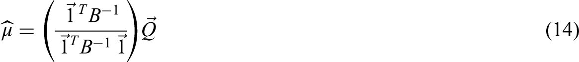
The best (i.e. with minimum variance) linear unbiased estimators of $μ$ and $σ$ are unique and are given by

{\hat{μ}}_{\vec{a}} = \frac{1}{Δ} [{\vec{α}}^{T} B^{- 1} (\vec{α} {\vec{1}}^{T} - \vec{1} {\vec{α}}^{T}) B^{- 1}] \vec{Q},

(8)

{\hat{σ}}_{\vec{b}} = \frac{1}{Δ} [{\vec{1}}^{T} B^{- 1} (\vec{1} {\vec{α}}^{T} - \vec{α} {\vec{1}}^{T}) B^{- 1}] \vec{Q},

(9)

where

Δ = ({\vec{1}}^{T} B^{- 1} \vec{1}) ({\vec{α}}^{T} B^{- 1} \vec{α}) - ({\vec{α}}^{T} B^{- 1} \vec{1})^{2} .

(10)

Moreover,

Var ({\hat{μ}}_{\vec{a}}) = σ^{2} \frac{{\vec{α}}^{T} B^{- 1} \vec{α}}{({\vec{1}}^{T} B^{- 1} \vec{1}) ({\vec{α}}^{T} B^{- 1} \vec{α}) - ({\vec{α}}^{T} B^{- 1} \vec{1})^{2}},

(11)

Var ({\hat{σ}}_{\vec{b}}) = σ^{2} \frac{{\vec{1}}^{T} B^{- 1} \vec{1}}{({\vec{1}}^{T} B^{- 1} \vec{1}) ({\vec{α}}^{T} B^{- 1} \vec{α}) - ({\vec{α}}^{T} B^{- 1} \vec{1})^{2}},

(12)

Cov ({\hat{μ}}_{\vec{a}}, {\hat{σ}}_{\vec{b}}) = - σ^{2} \frac{{\vec{α}}^{T} B^{- 1} \vec{1}}{({\vec{1}}^{T} B^{- 1} \vec{1}) ({\vec{α}}^{T} B^{- 1} \vec{α}) - ({\vec{α}}^{T} B^{- 1} \vec{1})^{2}} .

(13)

Proof.

We use the Lagrangian method and present the detailed proof in Appendix 6. with an alternative proof in Appendix 7. □

Theorem 2.2.

If the distribution is symmetric and the reported summaries are symmetric, the best (i.e., with minimum variance) linear unbiased estimators of $μ$ and $σ$ are

\hat{μ} = (\frac{{\vec{1}}^{T} B^{- 1}}{{\vec{1}}^{T} B^{- 1} \vec{1}}) \vec{Q}

(14)

\hat{σ} = (\frac{{\vec{α}}^{T} B^{- 1}}{{\vec{α}}^{T} B^{- 1} \vec{α}}) \vec{Q},

(15)

and their variances and covariance are given by

Var (\hat{μ}) = \frac{σ^{2}}{{\vec{1}}^{T} B^{- 1} \vec{1}}

, Var (\hat{σ}) = \frac{σ^{2}}{{\vec{α}}^{T} B^{- 1} \vec{α}}

, Cov (\hat{μ}, \hat{σ}) = 0

Proof.

It follows from Theorem 2.1 with the details presented in Appendix 6. □

2.2 Formulas for normal distribution and specific scenarios

In order to use the best linear estimators $\hat{μ}$ and $\hat{σ}$ given by (14) and (15), we need to calculate the vector $\vec{α}$ and the matrix $B$ .

Let $Y_{1 : n} < Y_{2 : n} < \dots < Y_{n : n}$ be order statistics from the standardized distribution with $μ = 0$ and $σ = 1$ . The coordinates of $\vec{α}$ are given by appropriate $E [Y_{r : n}]$ , while the diagonal entries of the matrix $B$ are given by appropriate $Var (Y_{r : n}) = E [Y_{r : n}^{2}] - (E [Y_{r : n}])^{2}$ and the off-diagonal entries by $Cov (Y_{r : n}, Y_{s : n}) = E [Y_{r : n} Y_{s : n}] - E [Y_{r : n}] E [Y_{s : n}]$ .

Explicit integral formulas are given in Appendix 5.. Those formulas can be used in a software package like R or Matlab, which can also be used to invert the matrix $B$ .

2.2.1. Scenario 1

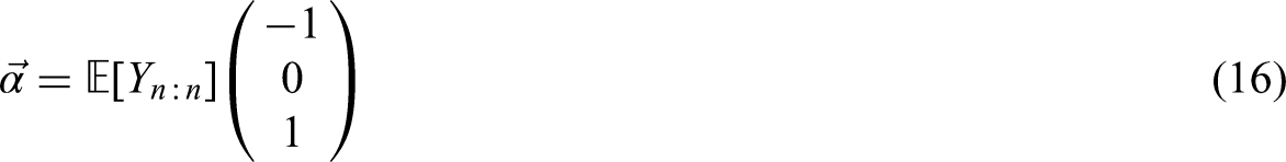
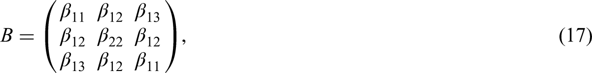
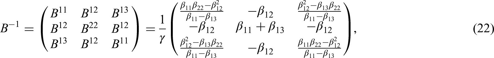
For illustration, we simplify formulas (14) and (15) for Scenario 1. Assume that the summary statistics consist of the minimum ( $Y_{1 : n}$ ), the median ( $Y_{\frac{n + 1}{2} : n}$ when $n$ is odd and $\frac{1}{2} (Y_{\frac{n}{2} : n} + Y_{\frac{n}{2} + 1 : n})$ when $n$ is even) and the maximum ( $Y_{n : n}$ ). For simplicity, we will deal only with odd $n$ . The calculations for even $n$ are analogs.

Due to the symmetry of the distribution

\vec{α} = E [Y_{n : n}] (\begin{matrix} - 1 \\ 0 \\ 1 \end{matrix})

(16)

and

B = (\begin{matrix} β_{11} β_{12} β_{13} \\ β_{12} β_{22} β_{12} \\ β_{13} β_{12} β_{11} \end{matrix}),

(17)

where

β_{11} = Var (Y_{n : n}) = E [Y_{n : n}^{2}] - (E [Y_{n : n}])^{2},

(18)

β_{12} = Cov (Y_{\frac{n + 1}{2} : n}, Y_{n : n}) = E [Y_{\frac{n + 1}{2} : n} Y_{n : n}] - E [Y_{\frac{n + 1}{2} : n}] E [Y_{n : n}] = E [Y_{\frac{n + 1}{2} : n} Y_{n : n}],

(19)

β_{13} = Cov (Y_{1 : n}, Y_{n : n}) = E [Y_{1 : n} Y_{n : n}] - E [Y_{1 : n}] E [Y_{n : n}],

(20)

β_{22} = Var (Y_{\frac{n + 1}{2} : n}) = E [Y_{\frac{n + 1}{2} : n}^{2}] - (E [Y_{\frac{n + 1}{2} : n}])^{2} = E [Y_{\frac{n + 1}{2} : n}^{2}] .

(21)

Let us first find the optimal estimator for

μ

from formula (14). We have,

B^{- 1} = (\begin{matrix} B^{11} & B^{12} & B^{13} \\ B^{12} & B^{22} & B^{12} \\ B^{13} & B^{12} & B^{11} \end{matrix}) = \frac{1}{γ} (\begin{matrix} \frac{β_{11} β_{22} - β_{12}^{2}}{β_{11} - β_{13}} & - β_{12} & \frac{β_{12}^{2} - β_{13} β_{22}}{β_{11} - β_{13}} \\ - β_{12} & β_{11} + β_{13} & - β_{12} \\ \frac{β_{12}^{2} - β_{13} β_{22}}{β_{11} - β_{13}} & - β_{12} & \frac{β_{11} β_{22} - β_{12}^{2}}{β_{11} - β_{13}} \end{matrix}),

(22)

where

γ = β_{11} β_{22} + β_{13} β_{22} - 2 β_{12}^{2}

. Thus,

{\vec{1}}^{T} B^{- 1} = \frac{1}{γ} (β_{22} - β_{12}, β_{11} - 2 β_{12} + β_{13}, β_{22} - β_{12}),

(23)

{\vec{1}}^{T} B^{- 1} \vec{1} = \frac{1}{γ} (2 β_{22} + β_{11} + β_{13} - 4 β_{12}) .

(24)

Consequently,

(\frac{{\vec{1}}^{T} B^{- 1}}{{\vec{1}}^{T} B^{- 1} \vec{1}}) = \frac{1}{2 β_{22} + β_{11} + β_{13} - 4 β_{12}} (β_{22} - β_{12}, β_{11} - 2 β_{12} + β_{13}, β_{22} - β_{12}) .

(25)

We note that the optimal linear unbiased estimator of

μ

in this scenario was developed in Luo et al.¹¹ and, by uniqueness, the estimators are identical.

Similarly, to find the optimal estimator for $σ$ from (15), we have

{\vec{α}}^{T} B^{- 1} = E [Y_{n : n}] (- 1, 0, 1) B^{- 1}

(26)

= E [Y_{n : n}] (B^{13} - B^{11}, B^{12} - B^{12}, B^{11} - B^{13})

(27)

= E [Y_{n : n}] (B^{11} - B^{13}) (- 1, 0, 1)

(28)

and thus

{\vec{α}}^{T} B^{- 1} \vec{α} = 2 E [Y_{n : n}]^{2} (B^{11} - B^{13}) .

(29)

Consequently,

(\frac{{\vec{α}}^{T} B^{- 1}}{{\vec{α}}^{T} B^{- 1} \vec{α}}) = (\frac{E [Y_{n : n}] (B^{11} - B^{13}) (- 1, 0, 1)}{2 E [Y_{n : n}]^{2} (B^{11} - B^{13})}) = \frac{1}{2 E [Y_{n : n}]} (- 1, 0, 1) .

(30)

Thus, the best estimator for

σ

given in (15) becomes

\hat{σ} = \frac{max - min}{2 E [max_{μ = 0, σ = 1}]} = \frac{Observed Range}{E [{Range}_{μ = 0, σ = 1}]},

(31)

where

E [max_{μ = 0, σ = 1}]

and

E [{Range}_{μ = 0, σ = 1}]

are the expected maximum and range from the standardized distribution with

μ = 0

and

σ = 1

, respectively. In the case of normal distribution, this estimator has been used since Tippett.⁵

2.3 Scenario 2

Assume that the summary statistics consist of the first quartile, the median and the third quartile. In the framework of this paper, the situation is analogs to Scenario 1. Thus, the best estimator for $σ$ given in (15) becomes

\hat{σ} = \frac{Observed (U Q - L Q)}{E [(U Q - L Q)_{μ = 0, σ = 1}]}

(32)

where

E [(U Q - L Q)_{μ = 0, σ = 1}]

is the expected difference between the upper and lower quartiles of the standardized distribution with

μ = 0

and

σ = 1

. In the case of normal distribution, this estimator has also already been used to estimate

σ

; see, for example, Wan et al.⁹

The optimal estimator for $μ$ is also analogs to Scenario 1 and it is the same as in Luo et al.¹¹

2.4 Scenario 3

Finally, assume that the summary statistics consist of the minimum, the first quartile, the median, the third quartile, and the maximum. As

\vec{α} = E [max μ = 0, σ = 1] (- 1, 0, 0, 0, 1) + E [U Q_{μ = 0, σ = 1}] (0, - 1, 0, 1, 0),

(33)

the best estimator for

σ

is an appropriately weighted average of estimators from Scenarios 1 and 2. Because both estimators, the one proposed here as well as the one proposed by Shi et al.,¹³ are optimal, it follows, by the uniqueness of the optimal estimators, that the two estimators are the same.

3 Simulation studies

3.1 Design of simulation studies

For illustration purposes, we consider the following seven scenarios for reported summary statistics:

Scenario 1:
min, median, max,
Scenario 2:
25% median, 75%,
Scenario 3:
min, 25%, median, 75%, max,
Scenario 4:
10%, median, 90%,
Scenario 5:
10%, 25%, median, 75%, 90%,
Scenario 6:
min, 10%, median, 90%, max,
Scenario 7:
min, 10%, 25%, median, 75%, 90%, max.
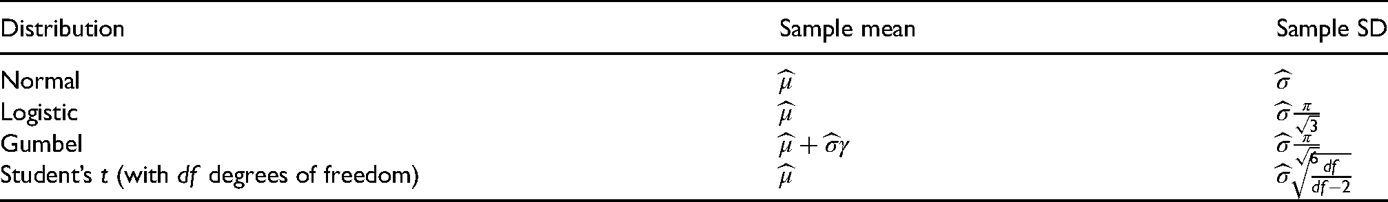
We consider the following four distributions: normal, logistic, Gumbel, and Student’s $t$ distribution (with 3, 5, 10, 20, or 30 degrees of freedom), all with location parameter $μ = 0$ and scale parameter $σ = 1$ . For each distribution, we generated $10^{4}$ samples of sizes $n \leq 1000$ . For each sample, we obtain the appropriate summary statistics and use these statistics to estimate $μ$ and $σ$ by (8) and (9), respectively. We record the bias and the mean squared error (MSE) of the estimates.
3.2 Results of simulation studies

The numerical simulations confirm that the estimators (8) and (9) are unbiased. Regardless of the scenario, distribution, or the sample size, the bias is generally between $- 0.01$ and $0.01$ for $μ$ and between $- 0.005$ and $0.005$ for $σ$ .

As expected, the MSE decreases with sample size.

There is also a difference between various scenarios. A scenario which reports more statistics gives a smaller MSE. In particular, from the seven scenarios we considered, Scenario 7 has the lowest MSE and Scenario 3 has MSE lower than either Scenario 1 or Scenario 2. This is easy to see from the optimality of the estimators. For example, the optimal estimator in Scenario 1 is also an estimator for Scenario 3 by simply ignoring the reported values of interquartile ranges. Thus, the optimal estimator for Scenario 3 will always have a strictly smaller MSE. This is seen in Figure 1.

Figure 1.

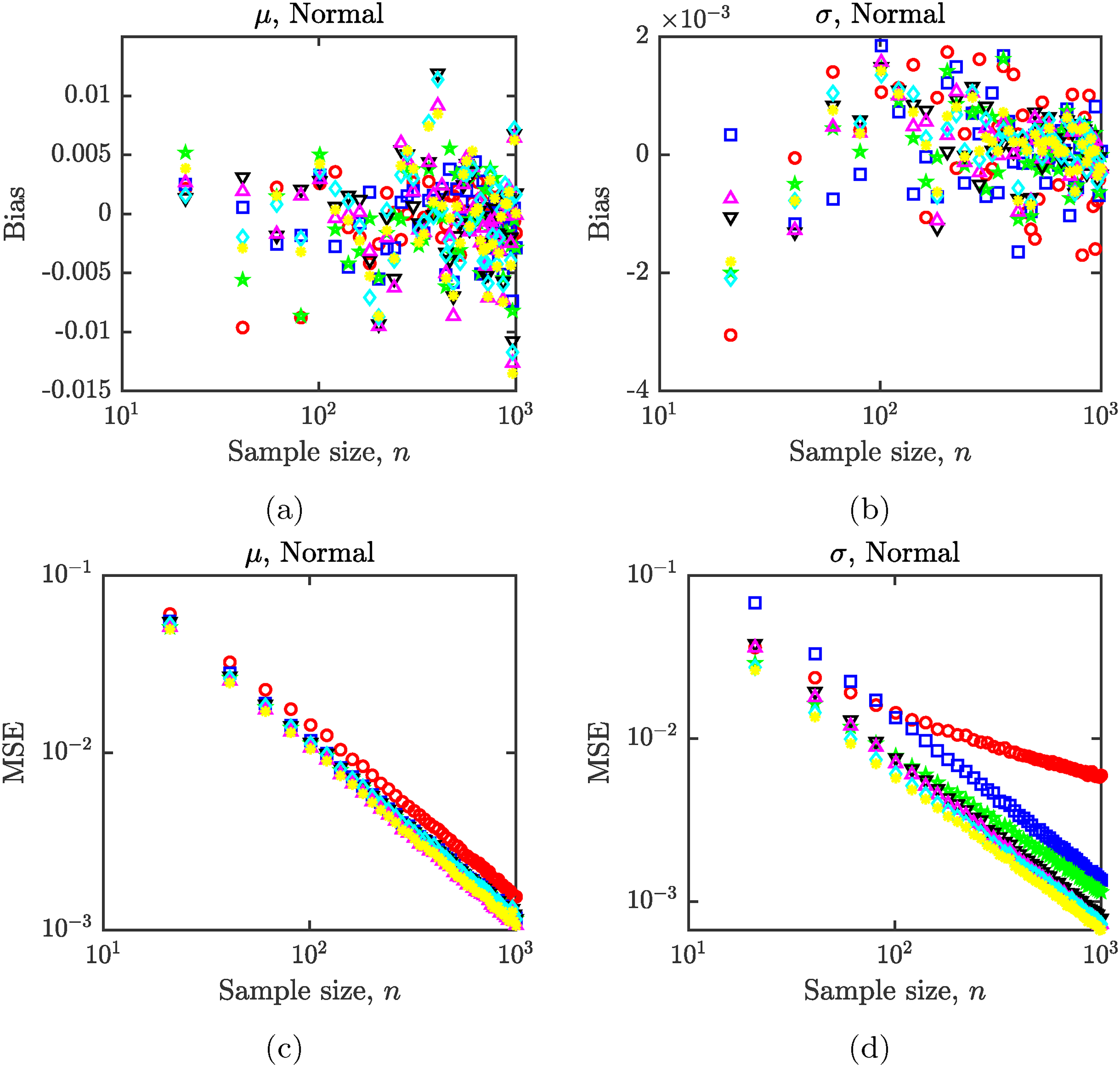
Bias (top row) and MSE (bottom row) for estimating $μ$ (left) and $σ$ (right) with normal distribution. Other considered distributions are analogous. Red circles—Scenario 1, blue squares—Scenario 2, green stars—Scenario 3, black triangles—Scenario 4, magenta triangles—Scenario 5, cyan diamonds—Scenario 6, yellow stars—Scenario 7.

An interesting observation is that when one scenario does not include all statistics reported by the other, the relationship between them depends on $n$ . This is visible especially for estimators of $σ$ . For example, in Scenario 1 we get a lower MSE than in Scenarios 2 and 4 for small $n$ , but the situation is reversed for larger $n$ . Similarly, in Scenario 3, we get lower MSE than Scenarios 4 or 5 for small $n$ , but higher MSE for larger $n$ . The reason is that the variation in the smallest and largest order statistics is small for small sample sizes; hence, they contribute relatively more information to the estimation of $σ$ in case of small $n$ . But, when $n$ becomes large, the variation in smallest and largest order statistics become too large (compared to interior order statistics, like quartiles) and so the estimation of $σ$ based on summary statistics including min and max become less efficient as compared to ones based on interior statistics.

3.3 Example of estimation of mean and SD

In this section, we illustrate the use of the proposed method to estimate the mean and SD when only summary statistics are reported. We note that the performance of the methods (for the normal distribution) have already been illustrated before.^11,13,14 Here, we use publicly available data from the Centers for Disease Control and Prevention on COVID-19 vaccination status in the US.²²For each US state (and territory), CDC provides 74 different statistics such as total doses delivered, doses delivered per 100K population, percentage of population with at least one dose, percentage fully vaccinated, etc. Data is also categorized by age (total or 18+) and vaccine (total, Pfitzer, Moderna, Janssen, unknown). When the data deals with absolute counts, it generally follows what seems to be a Gamma distribution with a skewness typically two or more. When data deals with percentages or with counts per 100K population, it generally follows an approximately normal distribution truncated between 0% and 100% or between 0 and the appropriate number of doses. The skewness is then around 0 or negative as the peak often occurs near the upper bound. This can be seen in Figure 2. 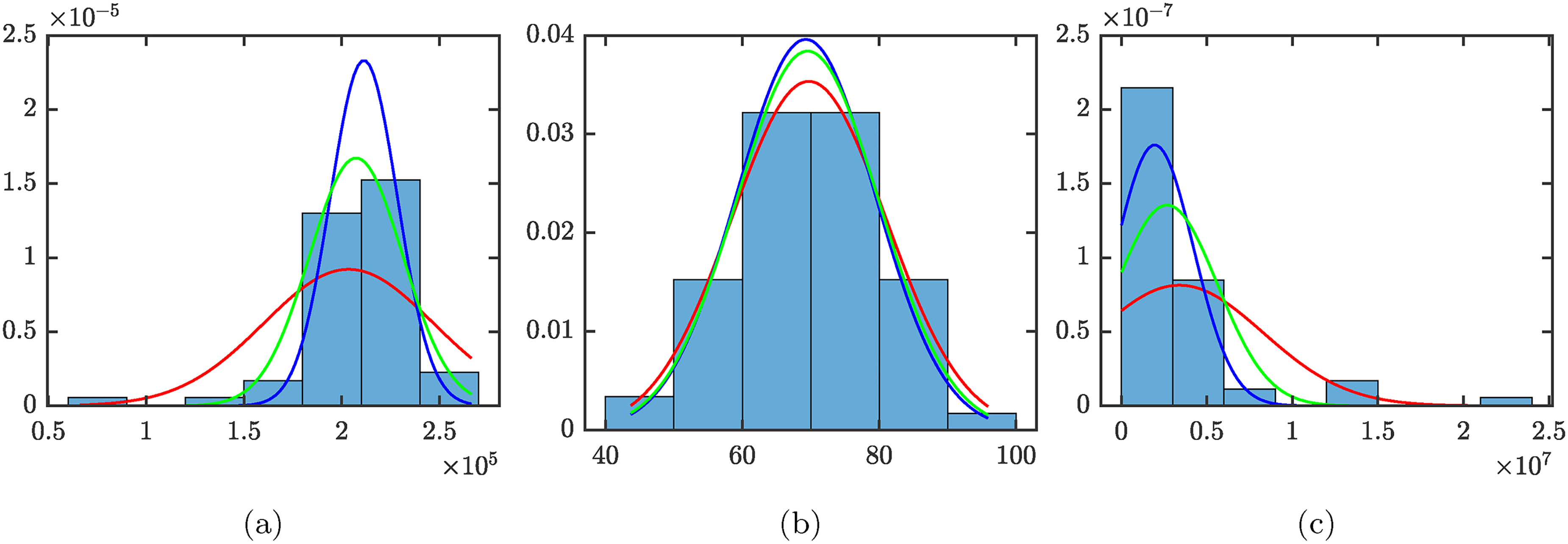For each of the provided statistics, we extracted the summaries for each scenario and used (8) and (9) to estimate the location parameter $μ$ and scale parameter $σ$ assuming the underlying distribution is normal, logistic, Gumbel or Student’s $t$ distribution (with 3, 5, 10, 20, or 30 degrees of freedom). We then used formulas from Table 1 to estimate the sample mean and sample SD.

Figure 2.

Representative histograms of the data sample from the CDC vaccination data²² and p.d.f.s of normal distributions obtained by estimating the mean and standard deviation (red: Scenario 1, blue: Scenario 2, green: Scenario 3). (a) The number of doses administered in each state per 100K of 65+ residents; (b) percentage of people 18+ in each state that are fully vaccinated; and (c) number of people 18+ in each state that are fully vaccinated. The skewness from left to right is $- 2.23$ , 0.09, and 2.78.

Table 1.

The mean and SD of sample of size $n$ from the specified distributions with the location parameter $μ$ and scale parameter $σ$ . For the Gumbel distribution, $γ \approx 0.57721$ is the Euler–Mascheroni constant.

Distribution	Sample mean	Sample SD
Normal	$\hat{μ}$	$\hat{σ}$
Logistic	$\hat{μ}$	$\hat{σ} \frac{π}{\sqrt{3}}$
Gumbel	$\hat{μ} + \hat{σ} γ$	$\hat{σ} \frac{π}{\sqrt{6}}$
Student’s $t$ (with $d f$ degrees of freedom)	$\hat{μ}$	$\hat{σ} \sqrt{\frac{d f}{d f - 2}}$

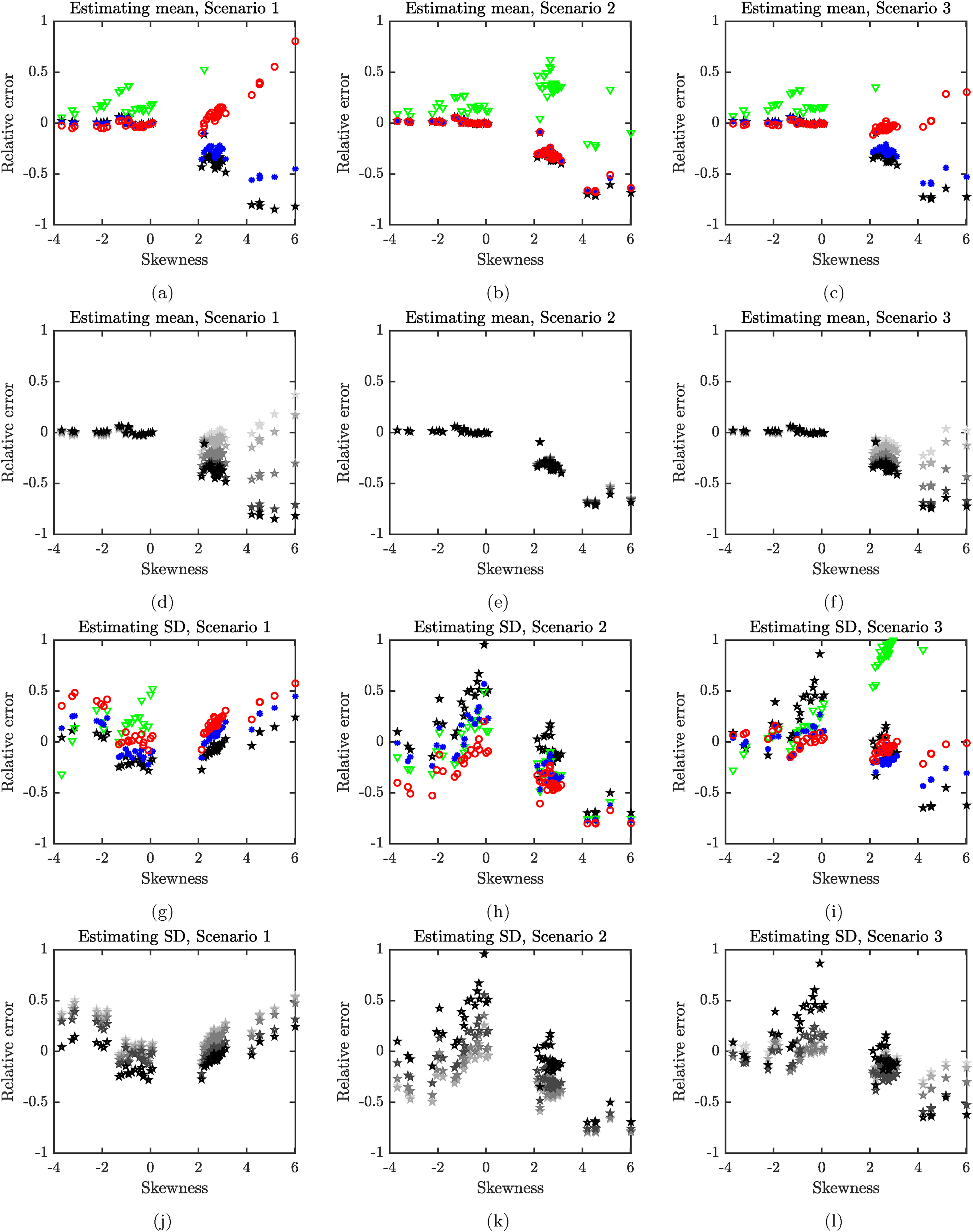
For normal estimates, as expected, the estimates of the mean and SD are very good for data that are close to normal. Moreover, the relative error of estimates of the mean are very low for all scenarios whenever the skewness is around $0$ . In Scenario 3, the relative errors are small even for samples with skewness under $4$ . In Scenario 1, the method overestimates the mean for samples with positive skewness. In Scenario 2, the method underestimates the mean for samples with positive skewness. The estimates of SD are quite good for samples with skewness close to 0 (or regardless of the skewness in Scenario 3). In Scenario 1, the method overestimates while in Scenario 2, the method underestimates the true SD whenever the sample skewness is not 0. The more asymmetrical the data are, the bigger is the difference between the true and estimated SD. This is illustrated in Figure 3.

Figure 3.

Relative error as it depends on the skewness of data. We estimate the mean and the standard deviation from the CDC vaccination data²² as if the underlying distribution is assumed to be normal (red circle), logistic (blue stars), Gumbel (green triangles), or Student’s $t$ (stars; black for $d f = 3$ and gradually getting lighter with increasing $d f \in {3, 5, 10, 20, 30}$ ). In most instances when the blue stars (or green triangles or black stars) are not visible, they are behind the red circles. However, in Scenario 3 for positive skewness, the error for Gumbel distribution is not displayed since it is larger than 1.

For our particular data sets, the estimates of the mean using logistic or Student’s $t$ distribution are similar to the normal estimates. When estimating the mean for samples with positive skewness, logistic or Student’s $t$ (with $d f = 10$ or $d f = 20$ ) estimates are slightly better in Scenario 1, but significantly underestimate in Scenario 3. Estimates using Gumbel distributions generally did not fare well.

4 Discussion

We proposed a general method to estimate the location parameter $μ$ and scale parameter $σ$ from reported summary statistics. The proposed method unifies the estimation of $μ$ and $σ$ which has so far been treated quite differently. The proposed estimators are linear, unbiased and have the lowest variance amongst all linear unbiased estimators. These estimates can then be used to estimate the sample mean and sample standard deviation from reported summary statistics. While we presented the method as a joint estimation of $μ$ and $σ$ , the method works and provides the best linear unbiased estimators even if one of the quantities $μ$ or $σ$ is reported with the data.

The proposed method has several advantages. First, it can be easily adapted to whatever summaries are reported without the need of extra theoretical derivations. In fact, the reported summaries do not even have to be symmetric. Second, the proposed method automatically gives the standard error. Finally, the method works for a general family of location-scale distributions, not only for normally distributed data. This includes the logistic, Laplace, Student’s $t$ , and Gumbel distributions. Moreover, the method can also be adopted for any log-location-scale family of distributions (like log-normal or Weibull distribution) since a log transformation, as discussed in Shi et al.,²³ will change it into a member of the location-scale family.

When data are skewed, investigators typically report the sample median and other sample quantiles, and so it is important to develop methods for this situation. Unfortunately, there is still a lack of literature on this subject with Shi et al.²³ and McGrath et al.²⁴ being notable exceptions. While the proposed method can handle non-normal data, the problem with a practical application of our method is that one needs to make a priori assumptions about the underlying data distribution. If the data distribution is not known, McGrath et al.²⁴ offer a promising approach of using the Box-Cox transformation to modify data summaries before estimating $μ$ and $σ$ . The Box-Cox transformation can be applied even in cases where the distribution is known but not of the type investigated in this paper, such as the beta distribution which fits the distribution of many clinical outcome variables.

Footnotes

Declaration of conflicting interests

The authors declared no potential conflicts of interest with respect to the research, authorship and/or publication of this article.

Funding

The research was funded by the Natural Sciences and Engineering Research Council of Canada RGPIN-2020-06733 (N.B.) and RGPIN/3670-2016 (S.D.W.). The funding agency had no input in study design, analysis and interpretation of data, in the writing of the report, nor in the decision to submit the article for publication.

ORCID iDs

Jan Rychtář

Stephen D Walter

Appendix A. Formulas

Appendix B. Proofs of the main theorems

Let $\vec{Q}$ be the vector of sample quantiles (need not be symmetric ones) from an unknown distribution $F$ (need not be symmetric) with a location parameter $μ$ and scale parameter $σ$ . Then, we have $E [\vec{Q}] = μ \vec{1} + σ \vec{α}$ and $Var (\vec{Q}) = σ^{2} B$ , where $\vec{α}$ is the mean vector for the standardized distribution and $B$ is variance-covariance matrix for the given summary statistics vector $\vec{Q}$ for the standardized distribution. Note that $B$ is symmetric (i.e. $B^{T} = B$ ) and positive-definite. Thus, $B^{- 1}$ exists and is symmetric (i.e. $(B^{- 1})^{T} = B^{- 1}$ ).

So, let us take the linear estimators of $μ$ and $σ$ to be ${\hat{μ}}_{\vec{a}} = {\vec{a}}^{T} \vec{Q}$ and ${\hat{σ}}_{\vec{b}} = {\vec{b}}^{T} \vec{Q}$ , where $\vec{a}$ and $\vec{b}$ are vectors that need to be determined optimally. Clearly, (47)

E [{\hat{μ}}_{\vec{a}}] = {\vec{a}}^{T} E [\vec{Q}] = μ {\vec{a}}^{T} \vec{1} + σ {\vec{a}}^{T} \vec{α},

(48)

E [{\hat{σ}}_{\vec{b}}] = {\vec{b}}^{T} E [\vec{Q}] = μ {\vec{b}}^{T} \vec{1} + σ {\vec{b}}^{T} \vec{α},

(49)

Var ({\hat{μ}}_{\vec{a}}) = σ^{2} {\vec{a}}^{T} B \vec{a},

(50)

Var ({\hat{σ}}_{\vec{b}}) = σ^{2} {\vec{b}}^{T} B \vec{b},

(51)

Cov ({\hat{μ}}_{\vec{a}}, {\hat{σ}}_{\vec{b}}) = σ^{2} {\vec{a}}^{T} B \vec{b} .

First, let us give necessary and sufficient conditions for the linear estimators

{\hat{μ}}_{\vec{a}}

and

{\hat{σ}}_{\vec{b}}

to be unbiased.

Now, let us minimize the trace, that is, the sum of variances (after dropping the multiple $σ^{2}$ ), given by ${\vec{a}}^{T} B \vec{a} + {\vec{b}}^{T} B \vec{b}$ subject to the unbiasness conditions ${\vec{a}}^{T} \vec{1} = 1$ , ${\vec{a}}^{T} \vec{α} = 0$ , ${\vec{b}}^{T} \vec{1} = 0$ and ${\vec{b}}^{T} \vec{α} = 1$ . So, for the Lagrangian method, let us consider the objective function (52)

L (\vec{a}, \vec{b}) = {\vec{a}}^{T} B \vec{a} + {\vec{b}}^{T} B \vec{b} - 2 λ_{1} ({\vec{a}}^{T} \vec{1} - 1) - 2 λ_{2} ({\vec{a}}^{T} \vec{α} - 0) - 2 λ_{3} ({\vec{b}}^{T} \vec{1} - 0) - 2 λ_{4} ({\vec{b}}^{T} \vec{α} - 1) .

Differentiating with respect to

\vec{a}

and

\vec{b}

, we get (53)

\frac{\partial L}{\partial \vec{a}} = 2 B \vec{a} - 2 λ_{1} \vec{1} - 2 λ_{2} \vec{α} = 0,

(54)

\frac{\partial L}{\partial \vec{b}} = 2 B \vec{b} - 2 λ_{3} \vec{1} - 2 λ_{4} \vec{α} = 0 .

From (53), we get

B \vec{a} = λ_{1} \vec{1} + λ_{2} \vec{α}

and thus, since

B

is positive definite, (55)

\vec{a} = λ_{1} B^{- 1} \vec{1} + λ_{2} B^{- 1} \vec{α} .

Therefore, we have (56)

{\vec{a}}^{T} \vec{1} = λ_{1} {\vec{1}}^{T} B^{- 1} \vec{1} + λ_{2} {\vec{α}}^{T} B^{- 1} \vec{1} = 1,

(57)

{\vec{a}}^{T} \vec{α} = λ_{1} {\vec{1}}^{T} B^{- 1} \vec{α} + λ_{2} {\vec{α}}^{T} B^{- 1} \vec{α} = 0 .

Thus, (58)

(\begin{matrix} λ_{1} \\ λ_{2} \end{matrix}) = {(\begin{matrix} {\vec{1}}^{T} B^{- 1} \vec{1} {\vec{α}}^{T} B^{- 1} \vec{1} \\ {\vec{α}}^{T} B^{- 1} \vec{1} {\vec{α}}^{T} B^{- 1} \vec{α} \end{matrix})}^{- 1} (\begin{matrix} 1 \\ 0 \end{matrix})

(59)

= \frac{1}{Δ} (\begin{matrix} {\vec{α}}^{T} B^{- 1} \vec{α} - {\vec{α}}^{T} B^{- 1} \vec{1} \\ - {\vec{α}}^{T} B^{- 1} \vec{1} {\vec{1}}^{T} B^{- 1} \vec{1} \end{matrix}) (\begin{matrix} 1 \\ 0 \end{matrix})

(60)

= \frac{1}{Δ} (\begin{matrix} {\vec{α}}^{T} B^{- 1} \vec{α} \\ - {\vec{α}}^{T} B^{- 1} \vec{1} \end{matrix}),

where (61)

Δ = ({\vec{1}}^{T} B^{- 1} \vec{1}) ({\vec{α}}^{T} B^{- 1} \vec{α}) - ({\vec{α}}^{T} B^{- 1} \vec{1})^{2} .

Now, substituting for

λ_{1}

and

λ_{2}

in (55), we obtain (62)

{\hat{μ}}_{\vec{a}} = {\vec{a}}^{T} \vec{Q} = λ_{1} {\vec{1}}^{T} B^{- 1} \vec{Q} + λ_{2} {\vec{α}}^{T} B^{- 1} \vec{Q}

(63)

= \frac{1}{Δ} (({\vec{α}}^{T} B^{- 1} \vec{α}) {\vec{1}}^{T} B^{- 1} \vec{Q} - ({\vec{α}}^{T} B^{- 1} \vec{1}) {\vec{α}}^{T} B^{- 1} \vec{Q})

(64)

= \frac{1}{Δ} {\vec{α}}^{T} B^{- 1} (\vec{α} {\vec{1}}^{T} - \vec{1} {\vec{α}}^{T}) B^{- 1} \vec{Q} .

Similarly, from (54), we get

B \vec{b} = λ_{3} \vec{1} + λ_{4} \vec{α}

and thus, (65)

\vec{b} = λ_{3} B^{- 1} \vec{1} + λ_{4} B^{- 1} \vec{α} .

Therefore, we have (66)

{\vec{b}}^{T} \vec{1} = λ_{3} {\vec{1}}^{T} B^{- 1} \vec{1} + λ_{4} {\vec{α}}^{T} B^{- 1} \vec{1} = 0,

(67)

{\vec{b}}^{T} \vec{α} = λ_{3} {\vec{1}}^{T} B^{- 1} \vec{α} + λ_{4} {\vec{α}}^{T} B^{- 1} \vec{α} = 1 .

Thus, (68)

(\begin{matrix} λ_{3} \\ λ_{4} \end{matrix}) = {(\begin{matrix} {\vec{1}}^{T} B^{- 1} \vec{1} {\vec{α}}^{T} B^{- 1} \vec{1} \\ {\vec{α}}^{T} B^{- 1} \vec{1} {\vec{α}}^{T} B^{- 1} \vec{α} \end{matrix})}^{- 1} (\begin{matrix} 0 \\ 1 \end{matrix})

(69)

= \frac{1}{Δ} (\begin{matrix} {\vec{α}}^{T} B^{- 1} \vec{α} - {\vec{α}}^{T} B^{- 1} \vec{1} \\ - {\vec{α}}^{T} B^{- 1} \vec{1} {\vec{1}}^{T} B^{- 1} \vec{1} \end{matrix}) (\begin{matrix} 0 \\ 1 \end{matrix})

(70)

= \frac{1}{Δ} (\begin{matrix} - {\vec{α}}^{T} B^{- 1} \vec{1} \\ {\vec{1}}^{T} B^{- 1} \vec{1} \end{matrix}) .

Now, substituting for

λ_{3}

and

λ_{4}

in (65), we obtain (71)

{\hat{σ}}_{\vec{b}} = {\vec{b}}^{T} \vec{Q} = λ_{3} {\vec{1}}^{T} B^{- 1} \vec{Q} + λ_{4} {\vec{α}}^{T} B^{- 1} \vec{Q}

(72)

= \frac{1}{Δ} ((- {\vec{α}}^{T} B^{- 1} \vec{1}) {\vec{1}}^{T} B^{- 1} \vec{Q} + ({\vec{1}}^{T} B^{- 1} \vec{1}) {\vec{α}}^{T} B^{- 1} \vec{Q})

(73)

= \frac{1}{Δ} {\vec{1}}^{T} B^{- 1} (\vec{1} {\vec{α}}^{T} - \vec{α} {\vec{1}}^{T}) B^{- 1} \vec{Q},

where as before (74)

Δ = ({\vec{1}}^{T} B^{- 1} \vec{1}) ({\vec{α}}^{T} B^{- 1} \vec{α}) - ({\vec{α}}^{T} B^{- 1} \vec{1})^{2} .

The estimators

{\hat{μ}}_{\vec{a}}

and

{\hat{σ}}_{\vec{b}}

are unbiased because (75)

E [{\hat{μ}}_{\vec{a}}] = \frac{1}{Δ} [{\vec{α}}^{T} B^{- 1} (\vec{α} {\vec{1}}^{T} - \vec{1} {\vec{α}}^{T}) B^{- 1}] E [\vec{Q}]

(76)

= \frac{1}{Δ} [{\vec{α}}^{T} B^{- 1} (\vec{α} {\vec{1}}^{T} - \vec{1} {\vec{α}}^{T}) B^{- 1}] (μ \vec{1} + σ \vec{α})

(77)

\begin{aligned} = \frac{1}{Δ} [({\vec{α}}^{T} B^{- 1} \vec{α}) ({\vec{1}}^{T} B^{- 1} \vec{1}) μ + ({\vec{α}}^{T} B^{- 1} \vec{α}) ({\vec{1}}^{T} B^{- 1} \vec{α}) σ - ({\vec{α}}^{T} B^{- 1} \vec{1})^{2} μ \\ - ({\vec{α}}^{T} B^{- 1} \vec{α}) ({\vec{1}}^{T} B^{- 1} \vec{α}) σ] \end{aligned}

(78)

= \frac{1}{Δ} [({\vec{α}}^{T} B^{- 1} \vec{α}) ({\vec{1}}^{T} B^{- 1} \vec{1}) - ({\vec{α}}^{T} B^{- 1} \vec{1})^{2}] μ

(79)

= μ

and (80)

E [{\hat{σ}}_{\vec{b}}] = \frac{1}{Δ} [{\vec{1}}^{T} B^{- 1} (\vec{1} {\vec{α}}^{T} - \vec{α} {\vec{1}}^{T}) B^{- 1}] E [\vec{Q}]

(81)

= \frac{1}{Δ} [{\vec{1}}^{T} B^{- 1} (\vec{1} {\vec{α}}^{T} - \vec{α} {\vec{1}}^{T}) B^{- 1}] (μ \vec{1} + σ \vec{α})

(82)

\begin{aligned} = \frac{1}{Δ} [({\vec{1}}^{T} B^{- 1} \vec{1}) ({\vec{α}}^{T} B^{- 1} \vec{1}) μ + ({\vec{1}}^{T} B^{- 1} \vec{1}) ({\vec{α}}^{T} B^{- 1} \vec{α}) σ - ({\vec{1}}^{T} B^{- 1} \vec{α}) ({\vec{1}}^{T} B^{- 1} \vec{1}) μ \\ - ({\vec{1}}^{T} B^{- 1} \vec{α})^{2}) σ] \end{aligned}

(83)

= \frac{1}{Δ} [({\vec{1}}^{T} B^{- 1} \vec{1}) ({\vec{α}}^{T} B^{- 1} \vec{α}) - ({\vec{1}}^{T} B^{- 1} \vec{α})^{2})] σ

(84)

= σ .

Moreover, (85)

Var ({\hat{μ}}_{\vec{a}}) = σ^{2} {\vec{a}}^{T} B \vec{a} = σ^{2} {\vec{a}}^{T} (λ_{1} \vec{1} + λ_{2} \vec{α})

(86)

= σ^{2} λ_{1} = σ^{2} \frac{{\vec{α}}^{T} B^{- 1} \vec{α}}{({\vec{1}}^{T} B^{- 1} \vec{1}) ({\vec{α}}^{T} B^{- 1} \vec{α}) - ({\vec{α}}^{T} B^{- 1} \vec{1})^{2}},

(87)

Var ({\hat{σ}}_{\vec{b}}) = σ^{2} {\vec{b}}^{T} B \vec{b} = σ^{2} {\vec{b}}^{T} (λ_{3} \vec{1} + λ_{4} \vec{α}) = σ^{2} λ_{4}

(88)

= σ^{2} \frac{{\vec{1}}^{T} B^{- 1} \vec{1}}{({\vec{1}}^{T} B^{- 1} \vec{1}) ({\vec{α}}^{T} B^{- 1} \vec{α}) - ({\vec{α}}^{T} B^{- 1} \vec{1})^{2}},

(89)

Cov ({\hat{μ}}_{\vec{a}}, {\hat{σ}}_{\vec{b}}) = σ^{2} {\vec{a}}^{T} B \vec{b} = σ^{2} {\vec{a}}^{T} (λ_{3} \vec{1} + λ_{4} \vec{α}) = σ^{2} λ_{3}

(90)

= - σ^{2} \frac{{\vec{α}}^{T} B^{- 1} \vec{1}}{({\vec{1}}^{T} B^{- 1} \vec{1}) ({\vec{α}}^{T} B^{- 1} \vec{α}) - ({\vec{α}}^{T} B^{- 1} \vec{1})^{2}} .

Furthermore, when the distribution is symmetric, and the reported statistics are symmetric, we get (91)

α_{i} = - α_{k - i + 1}, i = 1, \dots, k,

and (92)

β_{i j} = β_{j i} = β_{k - i + 1, k - j + 1}, 1 \leq i, j \leq k,

that is, the matrix

B

is doubly symmetric. Thus, the matrix

B^{- 1}

is also doubly symmetric. It follows that, in the symmetric case,

{\vec{α}}^{T} B^{- 1} \vec{1} = {\vec{1}}^{T} B^{- 1} \vec{α} = 0

and thus the estimators reduce to (93)

{\hat{μ}}_{\vec{a}} = \frac{{\vec{1}}^{T} B^{- 1} \vec{Q}}{{\vec{1}}^{T} B^{- 1} \vec{1}},

(94)

{\hat{σ}}_{\vec{b}} = \frac{{\vec{α}}^{T} B^{- 1} \vec{Q}}{{\vec{α}}^{T} B^{- 1} \vec{α}},

and we get (95)

Var ({\hat{μ}}_{\vec{a}}) = \frac{σ^{2}}{{\vec{1}}^{T} B^{- 1} \vec{1}},

(96)

Var ({\hat{σ}}_{\vec{b}}) = \frac{σ^{2}}{{\vec{α}}^{T} B^{- 1} \vec{α}},

(97)

Cov ({\hat{μ}}_{\vec{a}}, {\hat{σ}}_{\vec{b}}) = 0 .

The fact that the optimal unbiased linear estimators are unique is a classical result.²⁸ We can also see the uniqueness directly from the proof presented here. The optimal estimators are obtained by minimizing

(\vec{Q} - μ \vec{1} - σ \vec{α})^{T} B^{- 1} (\vec{Q} - μ \vec{1} - σ \vec{α})

. The two linear equations for

μ

and

σ

have a non-singular coefficient matrix and so the solutions are unique.

Appendix C. Estimation with change of optimality criterion

Here we present an alternative proof of Theorem 2.1.

Suppose we define a new parameter (98)

θ = μ + σ

and consider a linear estimator for

θ

as (99)

{\hat{θ}}_{\vec{c}} = {\vec{c}}^{T} \vec{Q}

where the coefficient vector

\vec{c}

needs to be determined suitably. Then, (100)

E [{\hat{θ}}_{\vec{c}}] = {\vec{c}}^{T} E [\vec{Q}] = {\vec{c}}^{T} (μ \vec{1} + σ \vec{α}) = μ ({\vec{c}}^{T} \vec{1}) + σ ({\vec{c}}^{T} \vec{α}),

and if we require

\hat{θ}

to be unbiased for

θ

, then the unbiasedness conditions are (101)

{\vec{c}}^{T} \vec{1} = 1,

(102)

{\vec{c}}^{T} \vec{α} = 1 .

Next, (103)

Var ({\hat{θ}}_{\vec{c}}) = Var ({\vec{c}}^{T} \vec{Q}) = σ ({\vec{c}}^{T} B \vec{c}),

which we wish to minimize subject to unbiasedness conditions (101) and (102). By Lagrangian method, we consider the objective function as (104)

L^{*} (\vec{c}) = {\vec{c}}^{T} B \vec{c} - 2 λ_{1} ({\vec{c}}^{T} \vec{1} - 1) - 2 λ_{2} ({\vec{c}}^{T} \vec{α} - 1) .

Differentiating with respect to

\vec{c}

, we find (105)

\frac{d L^{*}}{d \vec{c}} = 2 B \vec{c} - 2 λ_{1} \vec{1} - 2 λ_{2} \vec{α} = 0,

thus (106)

\vec{c} = λ_{1} B^{- 1} \vec{1} + λ_{2} B^{- 1} \vec{α} .

Then, from (106), the unbiasedness condition (101) gives (107)

λ_{1} {\vec{1}}^{T} B^{- 1} \vec{1} + λ_{2} {\vec{α}}^{T} B^{- 1} \vec{1} = 1 .

Similarly, from (106), the unbiasedness condition (102) gives (108)

λ_{1} {\vec{1}}^{T} B^{- 1} \vec{α} + λ_{2} {\vec{α}}^{T} B^{- 1} \vec{α} = 1 .

The solutions for

(λ_{1}, λ_{2})

from equations (107) and (108) is (109)

(\begin{matrix} λ_{1} \\ λ_{2} \end{matrix}) = {(\begin{matrix} {\vec{1}}^{T} B^{- 1} \vec{1} {\vec{α}}^{T} B^{- 1} \vec{1} \\ {\vec{α}}^{T} B^{- 1} \vec{1} {\vec{α}}^{T} B^{- 1} \vec{α} \end{matrix})}^{- 1} (\begin{matrix} 1 \\ 1 \end{matrix})

(110)

= \frac{1}{Δ} (\begin{matrix} {\vec{α}}^{T} B^{- 1} \vec{α} - {\vec{α}}^{T} B^{- 1} \vec{1} \\ - {\vec{α}}^{T} B^{- 1} \vec{1} {\vec{1}}^{T} B^{- 1} \vec{1} \end{matrix}) (\begin{matrix} 1 \\ 1 \end{matrix})

(111)

= \frac{1}{Δ} (\begin{matrix} {\vec{α}}^{T} B^{- 1} \vec{α} - {\vec{α}}^{T} B^{- 1} \vec{1} \\ - {\vec{α}}^{T} B^{- 1} \vec{1} + {\vec{1}}^{T} B^{- 1} \vec{1} \end{matrix}) .

Upon substituting these expressions for

λ_{1}

and

λ_{2}

in (106), we obtain (112)

{\vec{c}}^{T} = λ_{1} {\vec{1}}^{T} B^{- 1} + λ_{2} {\vec{α}}^{T} B^{- 1}

(113)

= \frac{1}{Δ} [({\vec{α}}^{T} B^{- 1} \vec{α}) - ({\vec{α}}^{T} B^{- 1} \vec{1})] {\vec{1}}^{T} B^{- 1} + \frac{1}{Δ} [- ({\vec{α}}^{T} B^{- 1} \vec{1}) + ({\vec{1}}^{T} B^{- 1} \vec{1})] {\vec{α}}^{T} B^{- 1} .

Thus, (114)

{\hat{θ}}_{\vec{c}} = {\vec{c}}^{T} \vec{Q}

(115)

= \frac{1}{Δ} [{\vec{α}}^{T} B^{- 1} \vec{α} {\vec{1}}^{T} B^{- 1} \vec{Q} - {\vec{α}}^{T} B^{- 1} \vec{1} {\vec{1}}^{T} B^{- 1} \vec{Q}] + \frac{1}{Δ} [- {\vec{α}}^{T} B^{- 1} \vec{1} {\vec{α}}^{T} B^{- 1} \vec{Q} + {\vec{1}}^{T} B^{- 1} \vec{1} {\vec{α}}^{T} B^{- 1} \vec{Q}]

(116)

= \frac{1}{Δ} {\vec{α}}^{T} B^{- 1} (\vec{α} {\vec{1}}^{T} - \vec{1} {\vec{α}}^{T}) B^{- 1} \vec{Q} + \frac{1}{Δ} {\vec{1}}^{T} B^{- 1} (\vec{1} {\vec{α}}^{T} - \vec{α} {\vec{1}}^{T}) B^{- 1} \vec{Q}

(117)

= {\hat{μ}}_{\vec{a}} + {\hat{σ}}_{\vec{b}}

as presented in (64) and (73), respectively.

Thus, the same estimators ${\hat{μ}}_{\vec{a}}$ and ${\hat{σ}}_{\vec{b}}$ we derived also minimize $Var ({\hat{θ}}_{\vec{c}})$ as seen readily from (117). In fact, Balakrishnan and Rao²⁹ have established that the Best Linear Unbiased Estimators ${\hat{μ}}_{\vec{a}}$ and ${\hat{σ}}_{\vec{b}}$ similarly minimize many other choices of objective functions.

References

Higgins

JPT

Thomas

Chandler

et al. Cochrane Handbook for Systematic Reviews of Interventions. Hoboken, New Jersey: John Wiley & Sons, 2019.

Thatcher

De Campos

Bell

et al. Epoetin alpha prevents anaemia and reduces transfusion requirements in patients undergoing primarily platinum-based chemotherapy for small cell lung cancer. Br J Cancer 1999; 80: 396–402.

Capanni

Calella

Biagini

et al. Prolonged n-3 polyunsaturated fatty acid supplementation ameliorates hepatic steatosis in patients with non-alcoholic fatty liver disease: a pilot study. Aliment Pharmacol Ther 2006; 23: 1143–1151.

Austin

. Balance diagnostics for comparing the distribution of baseline covariates between treatment groups in propensity-score matched samples. Stat Med 2009; 28: 3083–3107.

Tippett

LHC

. On the extreme individuals and the range of samples taken from a normal population. Biometrika 1925; 17: 364–387.

Hozo

Djulbegovic

Hozo

. Estimating the mean and variance from the median, range, and the size of a sample. BMC Med Res Methodol 2005; 5: 13.

Walter

Yao

. Effect sizes can be calculated for studies reporting ranges for outcome variables in systematic reviews. J Clin Epidemiol 2007; 60: 849–852.

Ramírez

Cox

. Improving on the range rule of thumb. Rose-Hulman Undergraduate Mathematics Journal 2012; 13: 1.

Wan

Wang

Liu

, et al. Estimating the sample mean and standard deviation from the sample size, median, range and/or interquartile range. BMC Med Res Methodol 2014; 14. Article number 135.

10.

Bland

. Estimating mean and standard deviation from the sample size, three quartiles, minimum, and maximum. Int J Stat Med Res 2015; 4: 57–64.

11.

Luo

Wan

Liu

, et al. Optimally estimating the sample mean from the sample size, median, mid-range, and/or mid-quartile range. Stat Methods Med Res 2018; 27: 1785–1805.

12.

Weir

Butcher

Assi

et al. Dealing with missing standard deviation and mean values in meta-analysis of continuous outcomes: a systematic review. BMC Med Res Methodol 2018; 18: 1–14.

13.

Shi

Luo

Weng

et al. Optimally estimating the sample standard deviation from the five-number summary. Res Synth Methods 2020; 11: 641–654.

14.

Rychtář

Taylor

. Estimating the sample variance from the sample size and range. Stat Med 2020; 39: 4667–4686.

15.

Weir

Assi

et al. Unreported summary statistics in trial publications and risk of bias in stroke rehabilitation systematic reviews: An international survey of review authors and examination of practical solutions. Journal of Stroke Medicine 2019; 2: 136–142.

16.

Eisenhauer

. Estimating sample means and standard deviations from quartiles and extrema. Journal of Probability and Statistical Science 2020; 18: 129–144.

17.

Eisenhauer

. A note on estimating unreported sample statistics for meta-analysis. Asian Journal of Probability and Statistics 2021; 13: 12–20.

18.

Walter

Rychtář

Taylor

, et al. Estimation of standard deviations and inverse-variance weights from an observed range. Stat Med 2022; 41: 242–257.

19.

Cai

Zhou

Pan

. Estimating the sample mean and standard deviation from order statistics and sample size in meta-analysis. Stat Methods Med Res 2021; 30: 2701–2719.

20.

Bowley

. An Elementary Manual of Statistics. London: Macdonald and Evans, 1920.

21.

Harter

Balakrishnan

. CRC Handbook of Tables for the Use of Order Statistics in Estimation. Florida: CRC Press, 1996.

22.

CDC. COVID Data tracker: COVID-19 Vaccinations in the United States. https://covid.cdc.gov/covid-data-tracker/vaccinations˙vacc-total-admin-admin-rate-total.

23.

Shi

Tong

Wang

, et al. Estimating the mean and variance from the five-number summary of a log-normal distribution. Stat Interface 2020; 13: 519–531.

24.

McGrath

Zhao

Steele

, et al. Estimating the sample mean and standard deviation from commonly reported quantiles in meta-analysis. Stat Methods Med Res 2020; 29: 2520–2537.

25.

Arnold

Balakrishnan

Nagaraja

. A First Course in Order Statistics. New York: John Willey and Sons, 1992.

26.

David

Johnson

. Statistical treatment of censored data part I. Fundamental formulae. Biometrika 1954; 41: 228–240.

27.

Arnold

Balakrishnan

. Relations, Bounds and Approximations for Order Statistics. New York: Springer Verlag, 1989.

28.

Rao

. Linear Statistical Inference and its Applications. vol. 2. New York: John Willey & Sons, 1973.

29.

Balakrishnan

Rao

. Some efficiency properties of best linear unbiased estimators. J Stat Plan Inference 2003; 113: 551–555.