
Abstract
The Brier score has been a popular measure of prediction accuracy for binary outcomes. However, it is not straightforward to interpret the Brier score for a prediction model since its value depends on the outcome prevalence. We decompose the Brier score into two components, the mean squares between the estimated and true underlying binary probabilities, and the variance of the binary outcome that is not reflective of the model performance. We then propose to modify the Brier score by removing the variance of the binary outcome, estimated via a general sliding window approach. We show that the new proposed measure is more sensitive for comparing different models through simulation. A standardized performance improvement measure is also proposed based on the new criterion to quantify the improvement of prediction performance. We apply the new measures to the data from the Breast Cancer Surveillance Consortium and compare the performance of predicting breast cancer risk using the models with and without its most important predictor.
Introduction
Developing a risk prediction model for binary outcomes has been very popular in clinical research and practice. For example, the Framingham risk score was developed to predict the ten-year risk of developing coronary heart disease. Since its first development, 1 the Framingham risk score has been validated in different population 2 and become a useful risk stratification tool for cardiovascular disease in clinical practice. The Breast Cancer Surveillance Consortium (BCSC) risk calculator was developed to predict a woman’s five-year risk of developing invasive breast cancer, 3 which is now commonly used for breast cancer screening in practice.
Guidelines on developing and validating risk prediction models have been discussed extensively in literature.4,5 A key exercise in developing a risk prediction model is to evaluate how well the model predicts the outcome. The performance of a prediction model is often evaluated in term of discrimination and calibration. For binary outcomes, discrimination refers to the model’s ability to separate those who developed the events from those who did not. Commonly used measures for model discrimination for binary outcomes include sensitivity, specificity, and C-statistic (i.e. the area under the receiver operating characteristic (ROC) curve).6–9 Calibration is a measure of how well the predicted probability of a binary outcome is in agreement with what was observed, which can be assessed by testing for lack-of-fit, such as the Hosmer-Lemeshow goodness-of-fit test. 10 More recent developments in the literature suggest evaluating the relationship between the observed outcome and corresponding predicted probabilities through graphical tools, 11 parametric models,12–14 and nonparametric smoothing methods. 15 Van Calster et al. 16 summarized different calibration measures using a hierarchy of four increasingly strict levels, referred to as mean, weak, moderate and strong calibration.
A prediction model that has good discrimination may not be well calibrated and vice versa. In addition to the discrimination and calibration evaluations, statistical measures for the overall prediction accuracy are also necessary. The Brier score has been a popular metric for evaluating the overall prediction accuracy of binary outcomes since it was introduced. 17 It is defined as the mean squared difference between the observed value of a binary outcome and its predicted probability. Despite its popularity in clinical prediction research, there are a few issues for interpreting the value of Brier score. For example, the C-statistic is a measure for model discrimination with values between 0.5 and 1. A larger C-statistic indicates better model discrimination and prediction performance. A rule of thumb is that a model with C-statistic greater than 0.8 is considered a well performing prediction model. Unlike the C-statistic, the Brier score is not defined in a standardized scale. Consequently, there is no single standard on how small the Brier score should be for a model with good prediction performance. Part of the reason is that the Brier score depends on the variance of the binary outcome, which is a function of the binary outcome probability. In this manuscript, we propose a decomposition of the Brier score, separating the part that measures the model prediction performance from the binary data variability determined by the underlying data generation mechanism. Since the data generation mechanism is unknown, it is difficult to have an unbiased estimate of the outcome variance. Therefore, our goal focuses on developing a measure that is more sensitive in comparing prediction performance than having an unbiased estimation.
Our work is partially motivated by the decomposition of Brier score literature. Two popular methods were proposed that partitioned the Brier score into either two 18 or three 19 components. In the three-component setting, each component corresponds to measures of the so-called reliability, resolution and uncertainty respectively. The uncertainty component is defined as the variance of a Bernoulli experiment with the probability of an event calculated as the average proportion of events occurred over all samples. It is calculated as if all subjects in the sample have the same probability of the binary outcome. However, the uncertainty component is not truly reflective of the data variability since different subjects may have different probabilities due to different covariate values. Instead, we propose to estimate the variability of the Bernoulli experiment for each subject and subtract it from the Brier score. The modified criterion is a pure measure of model performance such that its lower limit is zero when the true model is used.
We also propose a scaled measure based on the modified Brier score for comparing the prediction performance between different models. Similar work for modifying the Brier score to compare different models was done by Kattan and Gerds. 20 In their work, the Brier score was scaled by comparing to a null model in which there is no predictor. The model improvement was defined as the reduction of the Brier score relative to the null model.
The rest of the article is organized as follows. We first describe the proposed modified criterion, followed by its estimation in two different settings. We then describe two extensions of the modified criterion. We demonstrate the performance of the modified criterion through simulation with an application to the BCSC risk prediction. We conclude the article with a discussion and brief summary.
A modified criterion
Let
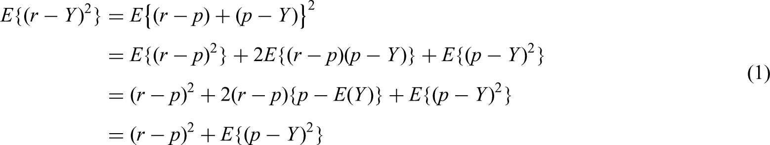
In the decomposition, the first component is the squared difference between the true and predicted probability of
For a total of

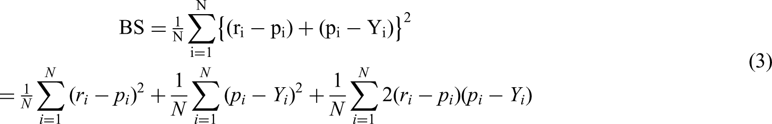

Similar to the Brier score, a smaller value of MSEP indicates a better prediction performance. The smallest possible value of MSEP is zero, when the true and predicted probabilities are exactly the same for all subjects. Since the true outcome probability is not known, the MSEP cannot be calculated directly. Instead, we propose to estimate the MSEP by subtracting the variance of
We propose a nonparametric method for estimating the binary outcome variance. Assume the predicted probabilities

Within each stratum
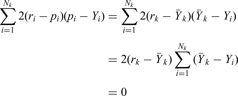
The MSEP can then be estimated as

When the number of unique predicted probabilities is large, the number of subjects within each stratum having the same predicted probabilities can be small so that
We first sort the outcome


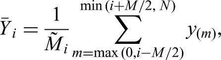
In practice, it is very difficult to have an unbiased estimate of the variance and MSEP accordingly, since we do not know the true data generation mechanism. It is preferred to have an underestimated variance as otherwise the MSEP may be negative when the variance is overestimated. As we will show through simulation in the next section, the estimated outcome variance and MSEP are not very sensitive to the sliding window size. In general, a smaller window size is preferred given the negative consequence of overestimating the variance.
The MSEP compares the difference between the true and predicted outcome probability. Sometimes, it may be useful to quantify the accuracy associated with the predicted probability relative to the true outcome probability. We can standardize the MSEP by taking its square root and then dividing by the outcome probability, referred to as the scaled root MSEP (SRMSEP), that is,

The performance improvement measure can also be defined using the Brier score. Suppose we redefine the performance improvement in equation (10) by replacing the MSEP with the Brier score. Let

We ran two simulation studies to evaluate the model prediction performance using the MSEP and compared it to the Brier score and index of prediction accuracy (IPA). 20
We generated a binary outcome

We fit two logistic models in the training data. The first model included
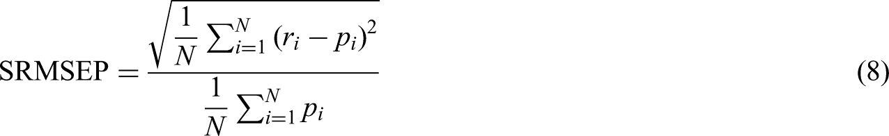
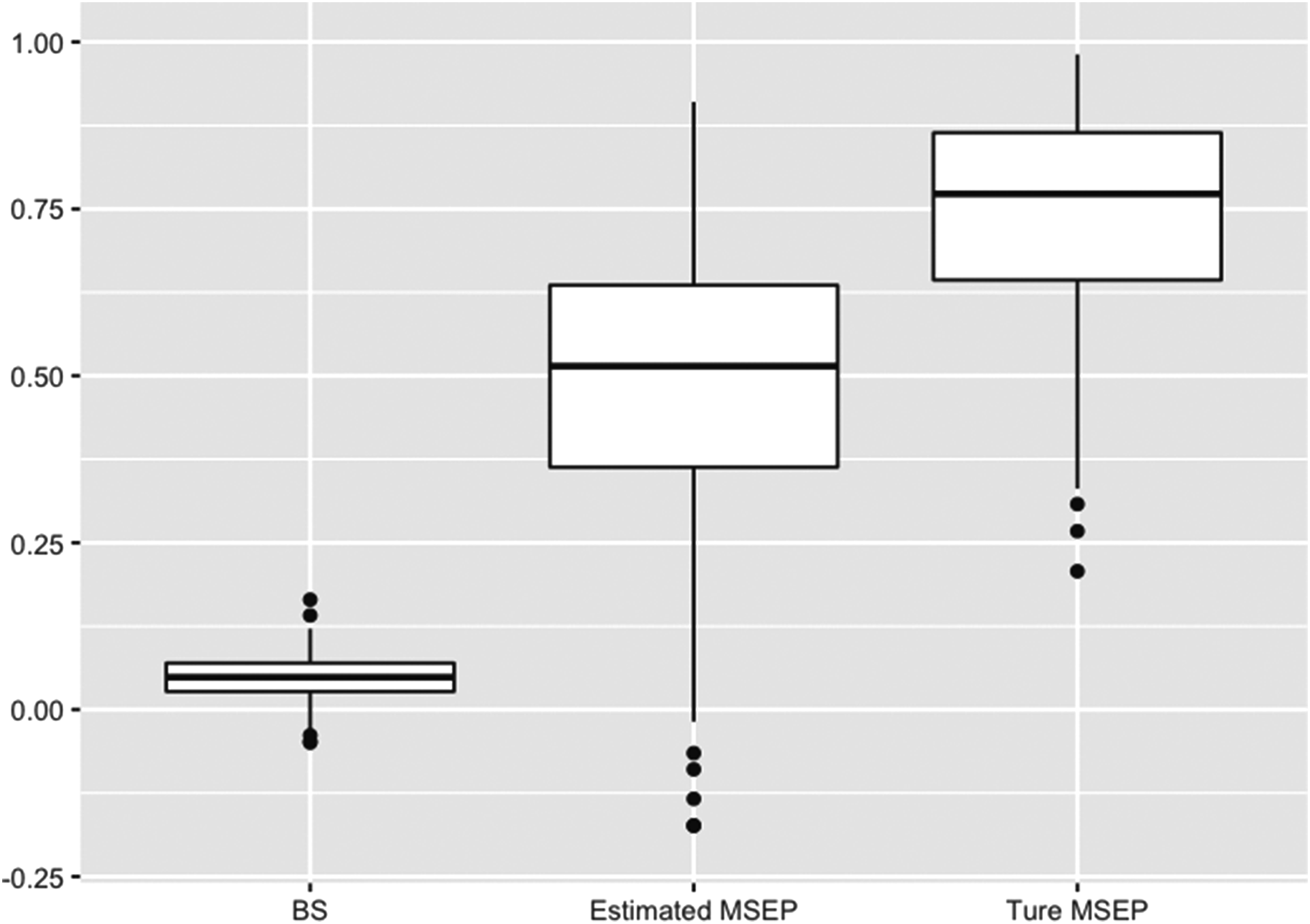
The comparison of BS, IPA, estimated and true MSEPs between the two models in Simulation I where all predictors are binary variables. MSEPs: mean square error for the probability of binary outcomes; BS: Brier score; IPA: index of prediction accuracy. Model 1 includes X 1 and X2 as the predictor. Model 2 additionally includes X 3 in the model.
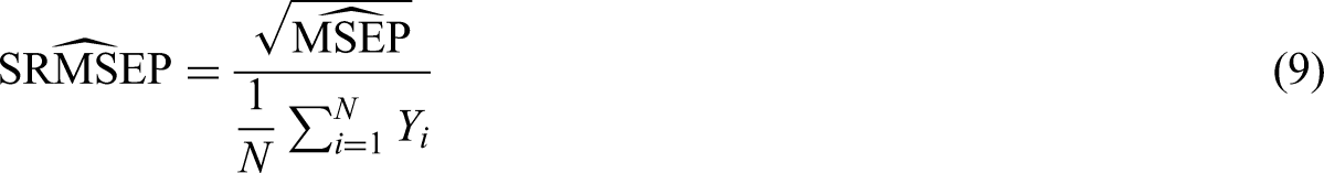
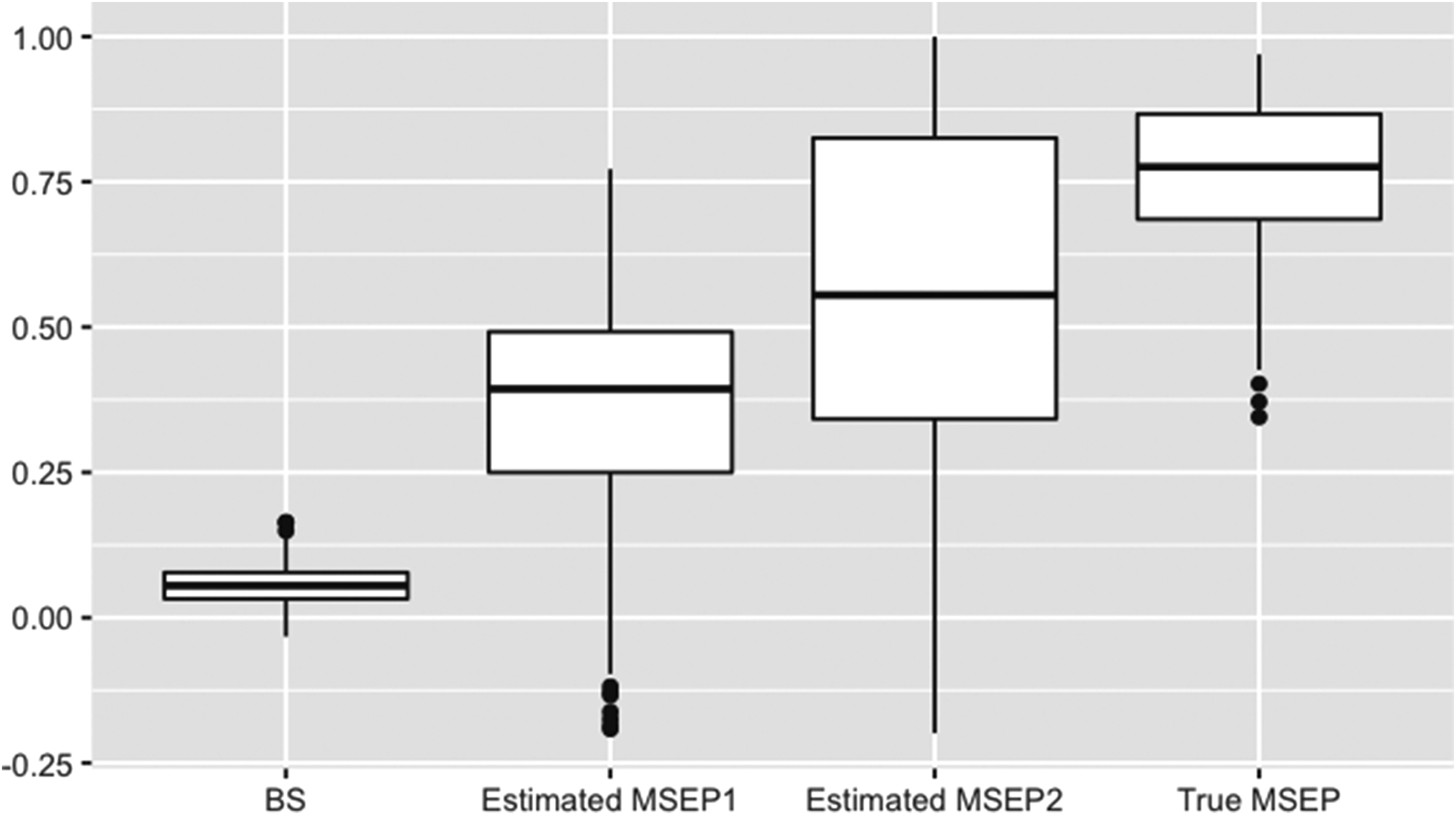
The comparison of BS, IPA, estimated and true MSEPs between the two models in Simulation II where all predictors are continuous variables. The MSEP1 and MSEP2 were estimated by ranking the subjects based on their predicted probabilities from Models 1 and 2, respectively. MSEPs: mean square error for the probability of binary outcome; BS: Brier score; IPA: index of prediction accuracy. Model 1 includes X 1 and X 2 as the predictor. Model 2 additionally includes X3 in the model.
Based on the second simulation, we additionally evaluated the sensitivity of the proposed variance estimator in equation (7) with respect to the moving average window size. We additionally increased the sample size of the validation data to 400 and 800. We also varied the
Figure 1 summarizes the results for the estimated BS, IPA, and MSEP for Simulation I. The distribution of the estimated BS and IPA for the two models overlapped, providing no clear evidence of model improvement by adding
Performance improvement between the two models defined using the BS, estimated and true MSEPs in Simulation I. MSEPs: mean square error for the probability of binary outcomes; BS: Brier score.
Figure 3 summarizes the results for the BS, IPA, and MSEPs for Simulation II. To evaluate if the estimated MSEP is sensitive to how the subjects were ordered in the sliding window approach, the MSEPs were estimated in two ways, differed by how the outcome variable was sorted. The outcomes were sorted by the predicted probabilities from Models 1 and 2 when estimating
Figure 4 shows the performance improvement comparing Models 1 and 2 in Simulation II, calculated using the BS, the two estimated MSEPs and true MSEP. The PI calculated using the two estimated MSEPs showed greater improvement compared to the one calculated using the Brier score, which is more consistent with the intuition that the prediction performance improves by adding an independent significant predictor.
Performance improvement between the two models defined using the BS, estimated and true MSEPs in Simulation II. The MSEP1 and MSEP2 were estimated by ranking the subjects based on their predicted probabilities from Models 1 and 2, respectively. MSEPs: mean square error for the probability of binary outcome; BS: Brier score.
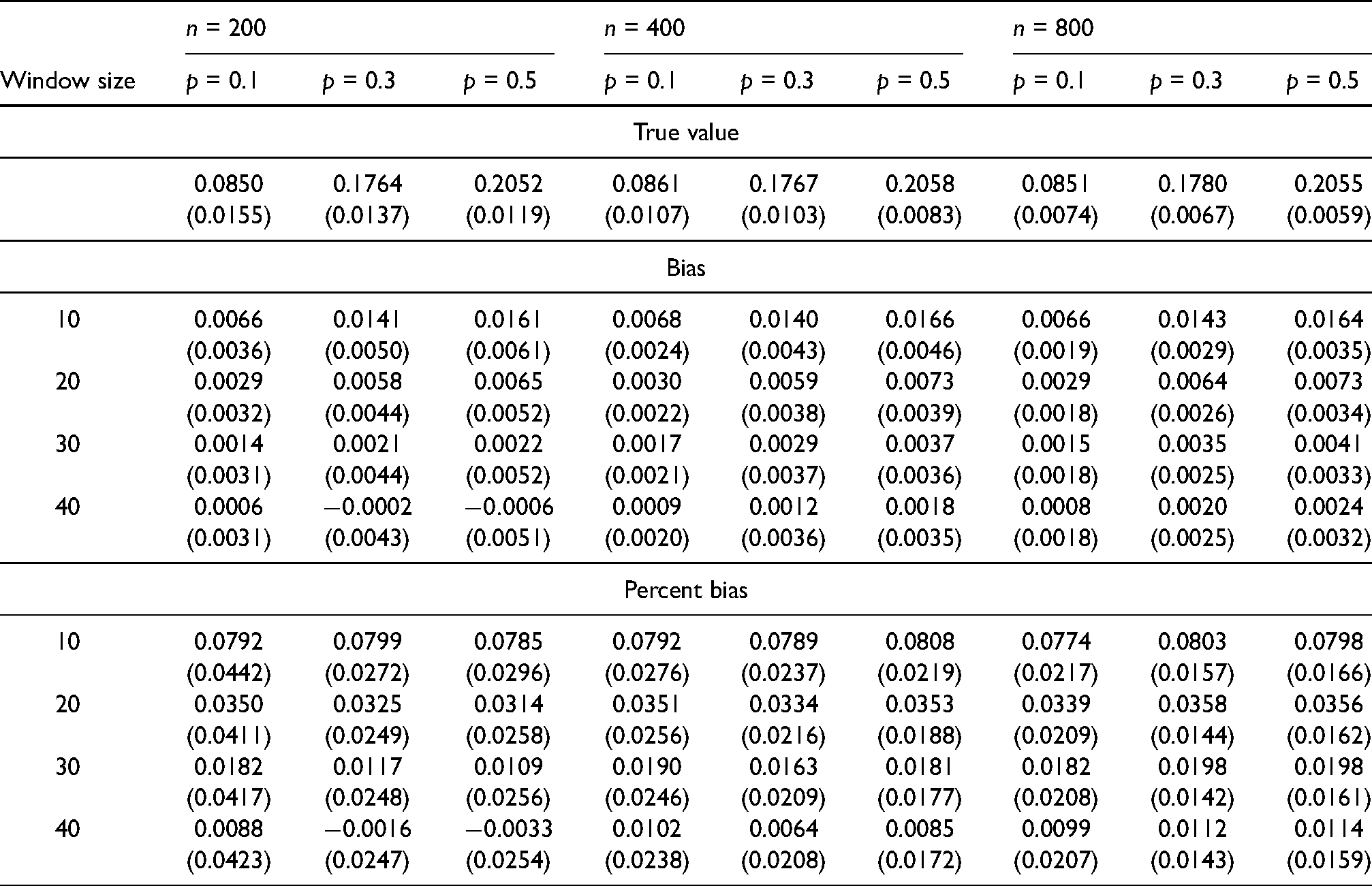
We evaluated the sensitivity of variance estimation with respect to the window size in Simulation II. Table 1 summarizes the bias and percent bias of the estimated outcome variance with varying window size under different sample sizes and outcome prevalences. In most scenarios, the bias reduces with increasing window size, although they are all relatively small. With fixed window size, the bias does not reduce with increasing total sample size. The largest bias is about 8% when the window size is 10. When the window size is relatively large compared to the total sample size (e.g. window size of 40 and total sample size of 200), the bias becomes negative, suggesting the variance is overestimated.
Mean (standard deviation) of the outcome variance, bias and percent bias of the estimated outcome variance across 200 simulations for different window size, total sample size and outcome prevalence. Bias is defined as the true minus estimated variance. Percent bias is defined as the true minus estimated variance divided by the true variance.
The Breast Cancer Surveillance Consortium (BCSC) was established in 1994 by the National Cancer Institute (NCI) to prospectively collect breast cancer risk factors at the time of each mammography screening, and ascertain outcomes for all women. 21 Using the BCSC dataset, Barlow et al. 22 developed a risk prediction model to estimate the probability of breast cancer diagnosis within one year after a screening mammogram. The model included race, ethnicity, breast density, BMI, use of hormone therapy, type of menopause, and previous mammographic result. The dataset included women aged between 35 and 84 years with mammograms screened from 1 January 1996 to 31 December 2002. There were 2,392,998 eligible screening mammograms from women who had not been previously diagnosed with breast cancer and had one prior mammogram in the preceding five years. Of those, 568,215 mammograms were from premenopausal women and 1726 were diagnosed with breast cancer within one year of the screening. The final model for premenopausal women included four predictors: age, breast density, number of first-degree relatives with breast cancer, and a prior breast procedure. Of the four predictors, breast density was the most significant predictor of breast cancer incidence.
Using four-fold cross validation method, we fit two logistic models: the model that included all predictors other than the breast density (Model 1) and the model with all four predictors (Model 2). Table 2 summarizes the comparison of the two models using different measures in the validation set. We first evaluated the performance of both models using the Brier score. The Brier scores are
Summary of prediction performance in the BCSC data. Model 1 included all predictors other than the breast density; model 2 included all four predictors. Since IPA is a relative measure with respect to the null model, the PI for the IPA is calculated as the difference of IPAs between the two models.
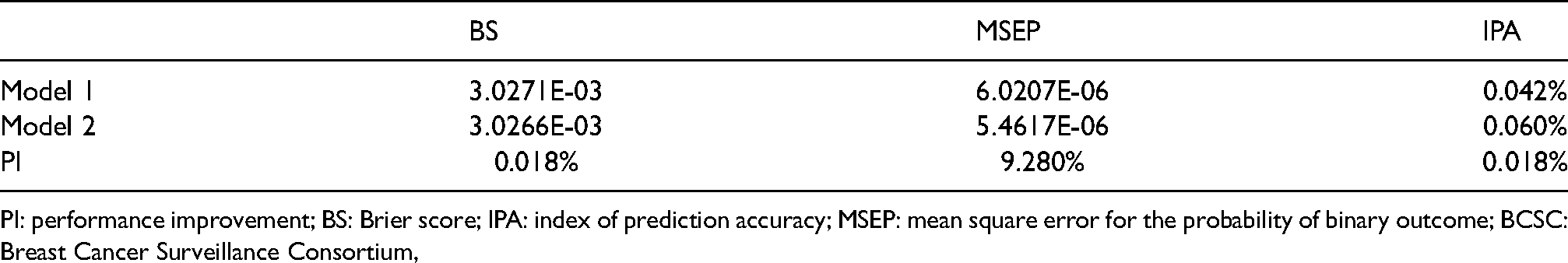
Summary of prediction performance in the BCSC data. Model 1 included all predictors other than the breast density; model 2 included all four predictors. Since IPA is a relative measure with respect to the null model, the PI for the IPA is calculated as the difference of IPAs between the two models.
PI: performance improvement; BS: Brier score; IPA: index of prediction accuracy; MSEP: mean square error for the probability of binary outcome; BCSC: Breast Cancer Surveillance Consortium,
We proposed a modified criterion based on the Brier score to evaluate and compare model performance for predicting binary outcomes. We decomposed the Brier score into the mean square error for the estimated probabilities and the intrinsic variance in the data. Since the variance of the binary outcome is not reflective of the model performance, we subtracted it from the Brier score and used only the first component, referred to as the MSEP, as the criterion for evaluating model performance. We showed the MSEP is more sensitive than the Brier score for quantifying the improvement when comparing the prediction performance of different models using the same dataset.
A key step in estimating the MSEP is to estimate the variance of binary outcomes. If the prediction model includes all categorical predictors, as was the case in the BCSC example, it is natural to group the subjects based on their predicted probabilities, which have a finite number of unique values, and calculate the variance for all subjects who have the same predicted probability. To handle the scenario of small number of subjects within each group, which is especially the case when there are continuous predictors in the model, we proposed a sliding window approach to estimate the variance for each subject by borrowing information from neighboring subjects who have similar outcome probabilities. The average outcome within the sliding window is a consistent estimator of the true outcome probability, a necessary condition for the product term in the Brier score decomposition to be zero.
A key parameter that needs to be specified is the window size when estimating the outcome variance using the sliding window approach. Using the simulation, we showed the estimated outcome variance is relatively insensitive to the window size. In the scenarios with a range of sample size and outcome prevalence, the largest bias is about 8%. We observed the bias reduces as the window size increases in most scenarios. However, in the few scenarios where the windows size is relatively large compared to the sample size (e.g. window size is 40 and sample size is 200), the bias is negative suggesting the variance is overestimated. Since we do not know the true model for the outcome, it is very difficult to have an unbiased estimate of the outcome variance. It is possible to develop an asymptotic procedure to have consistent estimate of the variance and MSEP accordingly, in which the optimal window size may depend on the sample size, outcome prevalence and other factors. Future research is required for selecting the optimal window size, which is beyond the scope of this work. In practice, a smaller window size is preferred as otherwise the proposed MSEP measure can be negative when the variance is overestimated (i.e. the Brier score is smaller than the estimated outcome variance). Consequently, we used the window size of 10 in both simulations and the BCSC data analysis. The sliding window approach is similar to the smoothing methods that have been used to estimate the calibration curve in literature. 15 Other methods may also be considered in estimating the outcome probability and associated variance, for example, kernel smoothing, repetitive sliding window. It will be interesting to see the comparison of performance using different methods in estimating the outcome variance, which can be another future direction of research.
A prediction model is meant to provide a tool for clinicians to improve decision-making in practice, which is not necessarily the true model for the relationship between predictors and outcome. To evaluate the performance of a new prediction model, it is important to compare it to a null model, 20 or a currently established model. On the other hand, it is also important to know the gap between the current model performance with respect to the “true” model, that is, how well can we predict the outcome using the existing data. Our proposed MSEP measure falls in the latter category. Since the expected MSEP is zero for the true model, the MSEP reflects the model performance with respect to the true model. It is complimentary to evaluate a candidate model by comparing it to both the null and “true” models.
Footnotes
Acknowledgements
The authors thank the anonymous reviewers and the editor for their constructive comments, which greatly improved the the manuscript.
Declaration of conflicting interests
The authors declared no potential conflicts of interest with respect to the research, authorship, and/or publication of this article.
Funding
The author(s) disclosed receipt of the following financial support for the research, authorship, and/or publication of this article: WY was supported by NIH R01-HL141294, R01-DK118079 and R01-HL161303; JJ was supported by NIH R01-HL141294 and NSFC grant 12101054; ES, and SK were supported by NIH R01-HL141294; WG was supported by NIH R01-HL141294, R01-DK117208, R01-HL161303 and R01-DK130067.