Standardization of continuous and categorical covariates in sparse penalized regressions

Abstract

In sparse penalized regressions, candidate covariates of different units need to be standardized beforehand so that the coefficient sizes are directly comparable and reflect their relative impacts, which leads to fairer variable selection. However, when covariates of mixed data types (e.g. continuous, binary or categorical) exist in the same dataset, the commonly used standardization methods may lead to different selection probabilities even when the covariates have the same impact on or level of association with the outcome. In this paper, we propose a novel standardization method that targets at generating comparable selection probabilities in sparse penalized regressions for continuous, binary or categorical covariates with the same impact. We illustrate the advantages of the proposed method in simulation studies, and apply it to the National Ambulatory Medical Care Survey data to select factors related to the opioid prescription in the US.

Keywords

Standardization dichotomization variable selection sparse penalized regression categorical covariates continuous covariates

1 Introduction

Impacts of covariates on the outcome are often measured by the corresponding coefficients in various regressions. Take linear regression as example, the impact of a covariate is often interpreted as the average or expected change in the outcome when the covariate changes by one unit or from the reference category to another category while holding all the other covariates constant. For continuous covariate, the coefficient size depends on its unit, where larger units lead to larger coefficients even when the impacts on or associations with the outcome remain the same. This creates difficulty in comparing the effect sizes of continuous covariates with different units. For instance, how to determine which factor has a bigger impact on the risk of diabetes, weight in pounds or BMI in kg/m $^{2}$ ? This issue becomes even more challenging when the covariates are of different types, for example, continuous covariates, binary covariates and categorical covariates with more than two levels. Their coefficients are interpreted in completely different ways and the coefficient sizes are not directly comparable. To be able to discuss and compare the impacts of covariates of different types, we first define covariate impact. We assume that all covariates, no matter what types (i.e. continuous, binary or categorical) they are when observed, are essentially generated from latent continuous variables. And we assume that the outcome is generated from an underlying model that is defined by the latent continuous variables and their relationships with the outcome could be linear, curved, step function, or mixture of discrete and continuous functions. Under this framework, we measure the covariate impacts using the effect sizes of the latent continuous covariates.

Sparse penalized regressions are often used to conduct simultaneous variable selection and coefficient estimation, where the coefficients are estimated by optimizing the penalized log-likelihood and are shrunk towards zero by the exerted penalty. However, one issue in performing the sparse penalized regressions in practice is that the covariates with higher probabilities of nonzero coefficient estimates do not necessarily have larger impacts on the outcome, especially when covariates are measured on different units or of different types. Therefore, in order to reduce the interference from different units or data types to the variable selection in sparse penalized regressions, it is important to standardize the covariates so that the standardized coefficients can reflect the covariate impacts. Consequently, penalized regression model applied on the standardized covariates would select covariates of larger impacts or stronger associations with higher chances, regardless of their units or data types.

It is a common practice to standardize covariates before carrying out sparse penalized regressions. In fact, the R package glmnet¹ for lasso and elastic net regression provides standardization option (True, False) and sets TRUE as default. The package ncvreg² for nonconvex penalties such as smoothly clipped absolute deviation (SCAD) and minimax concave penalty (MCP) only provides standardized coefficient estimates. Popular standardization approaches often implemented in the research works include Z-score,³ Gelman,⁴ Bring⁵ and Min–max.³ Z-score standardization is frequently applied in machine learning algorithms involving Euclidean distance measures, such as support vector machine, K-means, etc. It scales covariates by their sample standard deviations, so that the standardized covariate has a standard deviation equal to one. Based on the Z-score, Gelman⁴ made further adjustment which divides continuous covariates by twice their standard deviations and leaves binary and multi-category variables unmodified. This method improves the comparability between binary and continuous coefficients. Out of the same concern regarding the inconsistency of the standard deviations used in the Z-score method, Bring⁵ suggested to use partial standard deviation instead of marginal standard deviation. Since the marginal standard deviation measures the spread of the variable of interest for all observations in the sample without conditioning on the values of other covariates, which is not aligned with the regression coefficient that is interpreted under the condition that all other covariates are held constant. Min–max standardization maps continuous covariates proportionately to the range from zero to one, and makes no modification on the binary or multi-category covariates that are often represented by several binary indicators for different categories in comparison to the reference group. It’s popular in image processing and neural network models.⁶ We will review the details of those standardization approaches in the method section 2.1.

However, none of the standardization methods mentioned above specifically targets data with both continuous and categorical variables, and covariates essentially remain in different types, even after standardization since they still differ in ways beyond the first and second moments, especially for categorical data which is defined by much higher moments.⁷ As a result, standardized coefficients cannot reflect the covariate impacts, and the selection probabilities do not necessarily align with covariate impacts. For example, some standardization methods would favor continuous variables, while others prefer categorical variables, in terms of selection probabilities. In the present study, we propose a novel standardization method that aims at generating comparable selection probabilities for covariates of different types in the sparse penalized regression models. The strategy is to eliminate the essential difference across covariates of different types by dichotomizing continuous and multi-category covariates to binary variables, and leaving binary covariates unchanged, then scaling all binary covariates by their sample standard deviations, respectively. More details are given in the method section 2.1. Moreover, as there has always been controversial of using dichotomization,^8–10 we would like to emphasize that in the proposed standardization method, dichotomization serves as a tool to generate comparable coefficient sizes and fairer selection probabilities, not for the purpose of coefficient estimates or interpretations. When coefficient estimation is of concern, we recommend to fit the model using the original forms (before standardization) of the covariates, which are selected from the sparse penalized model applied on standardized inputs. We will address the issue in more details in the discussion section 5.

The remainder of the paper is organized as follows. In Section 2., we summarize the commonly implemented standardization approaches and detail the steps of the proposed standardization, followed by two theoretical results of the standardized coefficient estimates in the lasso logistic regressions. Next in Section 3., we conduct two sets of simulations to examine and compare how different standardization approaches perform with regard to generating comparable coefficient sizes and selection rates. Then in Section 4., we apply the group-lasso logistic regression on the 2016 National Ambulatory Medical Care Survey¹¹ (NACMS) data standardized by different standardization methods, screening for the important factors that drive opioid prescription in the US. Lastly in Section 5., we provide further discussions on the strengths and limitations of the proposed approach.

2 Method

2.1 Standardization

In this section, we explain the Z-score, Gelman, Bring and Min–max standardization methods through a simple example. Though coefficient interpretation is not our goal, it’s presented here to illustrate the connections among different standardization methods and to explain why the standardized coefficients are not comparable in some cases. Suppose a data set has two covariates and one outcome variable. One covariate is age ( $μ$ =30, sd=4), which is continuous with sample mean 30 and sample standard deviation four. The other covariate is gender, which is binary with zero for male and one for female. When there are equal number of males and females in the sample, the gender variable has mean and standard deviation both equal to 0.5. The outcome opioid is binary with one indicating that opioid is prescribed, zero otherwise. Fit a logistic regression $logit (P (o p i o i d = 1)) = β_{0} + β_{1} age + β_{2} \,female$ , and let ${\hat{β}}_{1}$ and ${\hat{β}}_{2}$ denote the maximum likelihood estimates of $β_{1}$ and $β_{2}$ .

When variables age and gender are in their original forms without any standardization, the interpretation of coefficient ${\hat{β}}_{1}$ would be, one year increment in age is expected to change the odds of having opioid prescribed by a multiplicative factor $e^{{\hat{β}}_{1}}$ , given the same gender. Similarly, with age fixed, females on average will have $e^{{\hat{β}}_{2}}$ times the odds of being prescribed opioid than the male group. However, a question often raised in practical setting is, which variable has larger impact on or stronger association with the probability of being prescribed opioid, age or gender? It certainly cannot be answered by comparing the sizes of ${\hat{β}}_{1}$ and ${\hat{β}}_{2}$ . Neither can we compare them using the P-values, which measure the probability of observing a coefficient estimate as extreme as or more extreme than ${\hat{β}}_{1}$ (or ${\hat{β}}_{2}$ ) when age (or gender) in fact has no impact, but does not measure the association strength between a covariate and the outcome.

Next we fit a logistic regression on the Z-score standardized covariates, age and gender are now on the same unit of one standard deviation and the corresponding coefficients are denoted as $α_{1}, α_{2}$ . The coefficient interpretation of ${\hat{α}}_{1}$ becomes, four years (one standard deviation) increment in age is expected to change the odds of opioid prescription by a multiplicative factor $e^{{\hat{α}}_{1}}$ , given the same gender. In a similar way, with age fixed, 0.5 (one standard deviation) increment in gender on average will lead to $e^{{\hat{α}}_{2}}$ folds change of the odds of opioid prescription. However, it does not make sense to have half change in a binary variable like gender, because there are only two meaningful values, zero for male and one for female, change in the amount of 0.5 has no practical meaning. Other than the interpretation problem in the presence of categorical covariates, Z-score standardization is sensitive to outliers. In the presence of small sample size or outliers, it’s possible that the standard deviation calculated from the sample does not approximate the population standard deviation well and leads to poorly scaled covariates, which can be partially remedied through robust standard deviation estimators such as inter-quartile range divided by 1.35.

The standardized coefficients calculated by the Bring⁵ method inherit the same interpretation and comparability issues as Z-score, but the Bring method makes a numerical improvement by using the partial standard deviation in the standardization, instead of the marginal standard deviation. The partial standard deviation is more appropriate than the marginal standard deviation because the former calculates the spread of the variable of interest conditioning on the values of other covariates, while the latter considers the spread of a variable for all observations in the sample. The partial standard deviation of variable $X$ is estimated by first regressing the variable on the other covariates to obtain the variance inflation factor (VIF), then calculated by equation $\frac{sd (X)}{\sqrt{vif (X)}} \sqrt{\frac{n - 1}{n - m}}$ , where $n, m$ are the number of observations and the number of covarites respectively. Additionally, the Bring standardized coefficient is related to the variables’s contribution to the outcome’s variance in terms of correlation of determination, when included in the regression.

In order to overcome the interpretation issue of Z-score standardization in the presence of binary covariates, Gelman⁴ suggested to scale the continuous variables by twice their standard deviations and leave the binary and multi-category variables unmodified. The rationale goes as follows, although it’s not reasonable to have one standard deviation (0.5) change in gender, it makes sense to have two standard deviations ( $2 \times 0.5 = 1$ ) change in gender, which is equivalent to using the original form of gender without any standardization. At the same time, continuous variables are scaled by two standard deviations, which enables the binary and continuous variables to be on the same unit of two standard deviations. However, this argument about the same unit depends on the probability of the binary covariate being one. If the probability lies between 0.3 and 0.7, the corresponding two standard deviations is between 0.92 and 1, close to 1. But when the probability is larger than 0.9 or smaller than 0.1, the two standard deviations is less than 0.6, quite different from 1, in which case the binary variables are no longer on the scale of two standard deviations as continuous variables.

Min–max standardization is popular in image processing, it does not modify the categorical variables, but linearly transforms continuous variable $X$ to the range $[0, 1]$ using the formula $\frac{x_{i} - min (X)}{max (X) - min (X)}$ , where $x_{i}$ is the value for the $i$ -th observation, $min (X)$ and $max (X)$ are the minimum and maximum values of $X$ in the observed data. When logistic regression is applied on the Min–max standardized data with coefficients denoted as $γ_{1}, γ_{2}$ , the interpretation of ${\hat{γ}}_{1}$ would be, the increment from the smallest age to the largest age across the sample is expected to change the odds of opioid prescription by a multiplicative factor $e^{{\hat{γ}}_{1}}$ , given the same gender. Since no transformation is exerted on the binary variable gender, ${\hat{γ}}_{2}$ has the same interpretation as ${\hat{β}}_{2}$ in the case where no standardization is used. That is, with age fixed, females on average will have $e^{{\hat{γ}}_{2}}$ times the odds of opioid prescription than the male group. The Min-max method is sensitive to outliers. When future sample falls outside the current range of the covariate, standardized covariate values will no longer be within $[0, 1]$ .

So far, all the standardization approaches mentioned above improve, but not address the comparability issue among coefficients of covariates of different types, which further leads to different selection probabilities in sparse penalized regressions even when the covariates have the same impact. To overcome this problem, we propose an alternative standardization method. Recall that we assume the relationship between the outcome and the observed covariate is in fact driven by the outcome’s relationship with a latent variable, and the covariate impact is measured by the corresponding latent effect size. The relationships between the latent covariates and the outcome are not necessarily linear, for example, it can be a polynomial function, step function, zero below a threshold then continuous after the threshold, etc. The observed covariates are generated from the latent continuous covariates by some mechanisms, for instance, the observed continuous covariate is the same as the latent continuous variable, the observed binary or multi-category covariate is categorized from the latent variable where categories correspond to non-overlapping regions of that latent variable. However, in practice, the latent variables are not observed and the mechanisms from the latent variables to observed covariates are often unknown, so it’s impossible to convert the observed variables back to the latent continuous variables. Nevertheless, we can always convert observed continuous covariates and multi-category covariates to binary variables, so that all the covariates are of binary types. And the coefficients of all binary covariates, which are essentially the differences between the average outcomes in two classes decided by the covariate values, would be comparable and reflect the covariate impacts to a certain degree. Furthermore, the comparability among coefficients would help sparse penalized regressions penalize covariate coefficients according to their relative impacts, leading to selection probabilities in agreement with impact sizes across continuous and categorical covariates. In summary, we propose to dichotomize the observed continuous and multi-category covariates using data-driven cutoff points and leave observed binary covariates unchanged, then standardize all binary variables by their standard deviations. More details are given in Section 2.2.

In the situations where data has no binary variables among the candidate covariates, there is no need to convert all continuous and categorical covariates into binary. Instead, we can convert the continuous covariates into the categorical variables with the fewest categories. For example, if the simplest categorical covariate has three levels—normal/overweight/obese, we would convert all continuous covariates (e.g. age) and categorical covariates with more than three levels (e.g. race) into three levels using the adaptive procedure with either random or empirical thresholds. The proposed standardization is not simply dichotomization. It is to eliminate the essential difference across covariates of different types by transforming all covariates into the same format, which is usually the simplest format, for example, the categorical variable with the fewest categories. However, if a data has only continuous covariates, no transformation is needed and we can directly standardize the continuous covariates using the Z-score method.

2.2 Steps of applying the proposed standardization

There are four steps to implement the proposed standardization, detailed as follows.

Identify the cutoff points using the $100 p$ -th percentiles. We use the $100 p$ -th percentiles as the cutoff points to dichotomize continuous covariates and regroup mutli-category covariates to binary variables, where $p$ is a data-driven value based on the observed binary covariates in a data set. Consider the empirical percentages of one in the observed binary covariates in the data, if the majority of probabilities are around certain value, we assign that value to $p$ ; otherwise, we set $p = 0.5$ . The purpose of choosing such cutoff points is to make dichotomized continuous and regrouped multi-category covariates consistent with the observed binary covariates in terms of the empirical probabilities of one.

Dichotomize continuous covariates to binary variables. The value of a continuous covariate is set to one if it’s less than the covariate’s $100 p$ -th percentile, otherwise it’s set to zero.

Regroup multi-category covariates to binary variables. For each multi-category covariate with $k (k > 2)$ levels, we first fit a regression model of the outcome on the multi-category variable alone, and conduct a likelihood-ratio test on the coefficients of all levels compared to the reference level. If the covariate effect is significantly different from zero, we regroup the levels to two new groups by the order of the coefficients. In detail, we rank the $k$ levels’ coefficients in ascending order and calculate the corresponding cumulative frequencies. Next we identify the level whose cumulative frequency is the closest to $p$ , then combine levels ranked lower than or equal to that level as one group, and combine higher levels as another group. If the likelihood-ratio test is not significant, we randomly rank the levels and follow the steps above to regroup the levels. The randomness is to prevent over-estimate of the effect of the newly constructed binary variable, when the underlying multi-category covariate has no effect on the outcome.

Standardize binary covariates by their standard deviations. Follow the same logic as in the Z-score standardization, dividing the binary covariate by one standard deviation can inflate the covariate values and deflate the coefficient estimate when the binary has extreme probability, hence achieving more comparable coefficient estimates among binary covariates of varying probabilities.

2.3. Group lasso logistic regression

There have been various types of sparse penalized regression models proposed in the last two decades, for instances, lasso regression,¹² elastic-net regression,¹³ etc. In the present study, we take a group-lasso logistic regression¹⁴ as an example to illustrate how different standardization methods affect variable selection in the sparse penalized regressions, especially when different types of variables (i.e. continuous, binary or categorical) coexist in a dataset.

Let $X_{n \times m}$ be the design matrix, $Y_{n \times 1}$ be the vector of binary responses, $β_{m \times 1}$ be the coefficients vector, where $n$ denotes the number of observations and $m$ denotes the number of covariates. The linear logistic regression models the conditional probability $P (Y = 1 | X_{i})$ using the logit transformation, $logit (P (Y = 1 | X_{i})) = η (X_{i})$ , where $η (X_{i}) = β_{0} + X_{i}^{T} β .$ When $X$ is standardized to $Z$ , the coefficient vector $β$ is denoted by $β^{s}$ , where $β^{s} = (β_{1}^{s}, \dots, β_{m}^{s})$ . The lasso logistic regression estimator $({\hat{β}}_{0}^{s}, {\hat{β}}^{s})$ is derived by minimizing the convex function

({\hat{β}}_{0}^{s}, {\hat{β}}^{s}) = \binom{argmin}{(β_{0}^{s}, β^{s})} [- l (β_{0}^{s}, β^{s}) + λ \sum_{j = 1}^{m} | β_{j}^{s} |]

(1)

where

l (β_{0}^{s}, β^{s}) = \sum_{i = 1}^{n} y_{i} η (Z_{i}) - \log [1 + \exp {η (Z_{i})}] .

In the objective function 1, the penalty term

λ \sum_{j = 1}^{m} | β_{j}^{s} |

shrinks the coefficient estimates towards zero¹² as

λ

increases. Meanwhile, the distributions of covariates also play a role in the probability of a covariate being selected. Therefore, standardization will influence coefficient estimates as well as the variable selection. In addition, in the presence of multi-category covariates, there are two drawbacks of using the lasso penalized regression. First, the variable selection is not robust to the choice of the reference groups of the multi-category variables. Second, when a multi-category covariate is represented by a set of dummy variables, lasso regression tends to select a subset instead of the entire set of dummy variables. We use the group-lasso penalized regression model proposed by Yuan and Lin,¹⁴ which overcomes the aforementioned concerns by selecting or eliminating entire sets of dummy variables using the objective function

({\hat{β}}_{0}^{s}, {\hat{β}}^{s}) = \binom{argmin}{(β_{0}^{s}, β^{s})} [- l (β_{0}^{s}, β^{s}) + λ \sum_{k = 1}^{K} \sqrt{m_{k}} ‖ β_{(k)}^{s} ‖],

where covariates are divided into

K

non-overlapping groups

{G_{k}, k = 1, \dots, K}

m_{k}

is the cardinality of the

k

-th group,

β_{(k)}^{s}

is the coefficients vector of covariates from the

k

-th group, and

‖ β_{(k)}^{s} ‖ = \sqrt{\sum_{j \in G_{k}} (β_{j}^{s})^{2}}

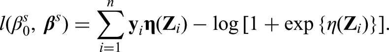
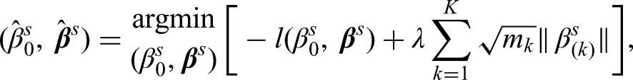
We provide two lemmas to theoretically justify that the proposed standardization will achieve fairer selection rates. Recall the assumption that each observed covariate is generated from a latent continuous covariate and that the covariate impacts to the outcome are reflected by the latent coefficients. Lemma 1 states that under certain conditions, applying the proposed standardization on covariates of different types will produce standardized coefficients that reflect the covariate impacts. Moreover, Lemma 2 states that under the same conditions, covariates with equal impacts have the same asymptotic probability of being selected in the lasso penalized logistic regression. Overall, Lemmas 1 and 2 together imply that applying the proposed standardization on covariates in logistic regression with lasso penalty will make fairer variable selection. The conclusion applies to group-lasso logistic regression and can be generalized to other types of linear regressions. The technique proofs of Lemmas 1 and 2 are provided in the Supplemental Material.

Lemma 1.

Suppose continuous variables $X_{1}, \dots, X_{m}$ are independent and have identical distribution $F$ . Outcome variable $Y$ is generated from Bernoulli $(1, π)$ with logit $(π) = β_{0} + β_{1} X_{1} + \dots + β_{m} X_{m}$ . Let $Z_{j} = I (X_{j} < F_{c}^{- 1} (p))$ , $j = 1, \dots, m$ and $p \in (0, 1)$ , where $F_{c}^{- 1} (\cdot)$ is the inverse of the cumulative distribution function of $F$ and $I (\cdot)$ is the indicator function. Fit a logistic regression of $Y$ on $Z_{1}, \dots, Z_{m}$ and denote the fitted coefficients as $α_{1}, α_{2}, \dots, α_{m}$ . If $β_{1} = β_{2} = \dots = β_{m}$ , $α_{1} = α_{2} = \dots = α_{m}$ . The conclusion also holds when $X_{1}, \dots, X_{m}$ have identical distributions and are correlated, with additional condition that the joint distribution is symmetric.

Lemma 2.

Suppose continuous variables $X_{1}, \dots, X_{m}$ are independent and have identical distribution. Outcome variable $Y$ follows Bernoulli $(1, π)$ with logit $(π) = β_{0} + β_{1} X_{1} + \dots + β_{m} X_{m}$ . Fit a lasso-penalized logistic regression of $Y$ on $X_{1}, \dots, X_{m}$ , if $β_{1} = β_{2} = \dots = β_{m}$ , the selection probabilities of variables $X_{1}, \dots, X_{m}$ are the same asymptotically.

3. Simulation study

We conduct two sets of simulation studies to compare the performance of the five standardization approaches discussed in Section 2.1., as well as the method of using covariates in their observed forms without standardization. In both simulations, we first generate latent continuous variables from multi-variate normal distribution, then create the response variable using logit link and latent variables with equal latent coefficients. This is a very special case of our hypothetical latent variables where all latent variables have the same distribution and the same effect size on the outcome, therefore, the impacts of all the covariates are the same. Next we construct the observed covariates by converting the latent variables to continuous, binary and multi-category forms. Last we standardize the observed covariates and fit logistic regression models without (simulation I) or with (simulation II) penalty. The first simulation assesses the statement in Lemma 1 and examines whether relationships among latent coefficients are retained after standardization, and the second simulation assesses the statement in Lemma 2 and shows how standardization affects variable selection in sparse penalized regressions. We use R package glmnet¹ to run regular logistic regression and packages gglasso¹⁵ and grplasso¹⁶ to perform group-lasso logistic regression, the last two packages allow us to use user-defined standardization and sampling weights.

3.1. Simulation I: recover covariate impacts with standardization

In simulation I, we examine whether the standardized coefficients mimic relationships among latent coefficients, which would indicate that the standardization is able to recover the relative impacts of the latent covariates on the outcome, that is, the covariates with larger latent coefficients would have larger standardized coefficients, representing more impacts or stronger associations, regardless of the types of observed covariates. We employ linear functions for the relationships between latent covariates and the logit outcome, and set the sizes of all latent coefficients to the same value. The observed covariates are generated from latent covariates to different types (continuous, binary and categorical). If we fit a regression model directly on the observed covariates, the sizes of the fitted coefficients are not equal. A good standardization method would maintain the equality among standardized coefficients, reflecting the equal relationship among the covariate impacts. Therefore, in the simulation we inspect if standardized coefficients remain equal for each standardization method.

The simulation setup is as follows.

Generate three latent continuous covariates $X_{n \times m} = (X_{1}, X_{2}, X_{3})$ from multivariate normal distribution $N (0_{m \times 1}, I_{m \times m})$ , where $I$ is the identity matrix, $n = 100$ and $m = 3$ .

Generate the binary outcome $Y$ by sampling from Bernoulli distribution with probability $\frac{\exp {η_{i}}}{1 + \exp {η_{i}}}$ , where $η_{i} = 2 X_{i 1} + 2 X_{i 2} + 2 X_{i 3}$ , $i = 1, \dots, n$ . As mentioned earlier, the coefficients of all latent covariates are of the same size.

Generate the observed covariates $(X_{c o n t}, X_{b i}, X_{m u l t i})$ .

c.1
$X_{c o n t} = X_{1}$ , $X_{c o n t}$ remains continuous;
c.2
$X_{b i} = I (X_{2} \leq Φ^{- 1} (q))$ , $X_{b i}$ is dichotomized from $X_{2}$ , where $I (\cdot)$ is the indicator function, $Φ (\cdot)$ denotes standard normal cumulative distribution function and $q \in {0.5, 0.7, 0.9}$ ;
c.3
$X_{m u l t i} = I (Φ^{- 1} (\frac{1}{3}) < X_{3} \leq Φ^{- 1} (\frac{2}{3})) + 2 \times I (Φ^{- 1} (\frac{2}{3}) < X_{3})$ , $X_{m u l t i}$ is trichotomized from $X_{3}$ and takes values in {0, 1, 2}.

Standardize the observed data $(X_{c o n t}, X_{b i}, X_{m u l t i})$ to $(Z_{c o n t}, Z_{b i}, Z_{m u l t i})$ using different standardization methods, then fit logistic regression of $Y$ on ( $Z_{c o n t}, Z_{b i}, Z_{m u l t i}$ ), and record the coefficient estimates and their ratios.
The setup is repeated 2000 times, and the results are reported in Table 1. There are three main columns indicating the $q$ values in converting latent $X_{2}$ to the observed binary $X_{b i}$ . For example, the first column has $q = 0.5$ , meaning that in step (c.2) $X_{b i}$ is dichotomized from the latent $X_{2}$ with $X_{b i} = I (X_{2} \leq Φ^{- 1} (q = 0.5))$ . The sub-column Coefficient Estimate lists the average standarized coefficients of $Z_{c o n t}$ and $Z_{b i}$ , and their empirical standard deviations in the parenthesis. The sub-column Ratio records the average ratio between the standardized coefficients of $Z_{c o n t}$ and $Z_{b i}$ , as well as their empirical standard deviations in the parenthesis. Each row section corresponds to the results of different standardization approaches. We report the average standardized coefficient of $Z_{m u l t i}$ and its coefficient ratio with $Z_{c o n t}$ only for the proposed standardization in the last row, since $Z_{m u l t i}$ in other methods contains multiple levels, while it is reduced to binary form under the proposed method.

Table 1.
Average standardized coefficient sizes (empirical standard deviation) of $Z_{c o n t}$ and $Z_{b i}$ , and the average ratios between their coefficient sizes (empirical standard deviation).

$q = 0.5$ $q = 0.7$ $q = 0.9$

Standardization Coefficient estimate Ratio Coefficient estimate Ratio Coefficient estimate Ratio

None

$Z_{c o n t}$ $^{a}$ 1.68 (0.43) 1.64 (0.43) 1.45 (0.36)

$Z_{b i}$ $^{a}$ 2.65 (0.72) 0.66 (0.15) 2.72 (0.89) 0.63 (0.16) 6.02 (6.55) 0.48 (0.12)

Z-score

$Z_{c o n t}$ 1.67 (0.44) 1.64 (0.44) 1.44 (0.38)

$Z_{b i}$ 1.33 (0.36) 1.30 (0.31) 1.25 (0.41) 1.37 (0.35) 1.82 (1.98) 1.59 (0.40)

Gelman

$Z_{c o n t}$ 3.35 (0.89) 3.27 (0.88) 2.89 (0.76)

$Z_{b i}$ 2.65 (0.72) 1.31 (0.31) 2.72 (0.90) 1.26 (0.32) 6.03 (6.56) 0.96 (0.24)

Min–max

$Z_{c o n t}$ 8.40 (2.36) 8.22 (2.35) 7.23 (2.02)

$Z_{b i}$ 2.65 (0.72) 3.28 (0.81) 2.72 (0.90) 3.17 (0.85) 6.04 (6.57) 2.39 (0.62)

Bring

$Z_{c o n t}$ 1.67 (0.44) 1.64 (0.44) 1.44 (0.38)

$Z_{b i}$ 1.33 (0.36) 1.30 (0.31) 1.25 (0.41) 1.37 (0.35) 1.82 (1.98) 1.58 (0.40)

Proposed

$Z_{c o n t}$ 2.15 (0.90) 1.95 (0.57) 2.94 (3.76)

$Z_{b i}$ 2.17 (0.89) 1.03 (0.28) $^{b}$ 1.93 (0.57) 1.05 (0.32) 3.11 (3.89) 1.07 (0.45)

$Z_{m u l t i}$ 2.06 (0.85) 1.03 (0.31) $^{c}$ 1.92 (0.66) 1.01 (0.30) 1.59 (0.67) 0.90 (0.38)

$^{a}$ Though no standardization is applied, here we use $Z_{c o n t}$ and $Z_{b i}$ to keep notation consistency.

$^{b}$ Ratio between coefficient of $Z_{c o n t}$ and coefficient of $Z_{b i}$ .

$^{c}$ Ratio between coefficient of $Z_{c o n t}$ and coefficient of $Z_{m u l t i}$ .

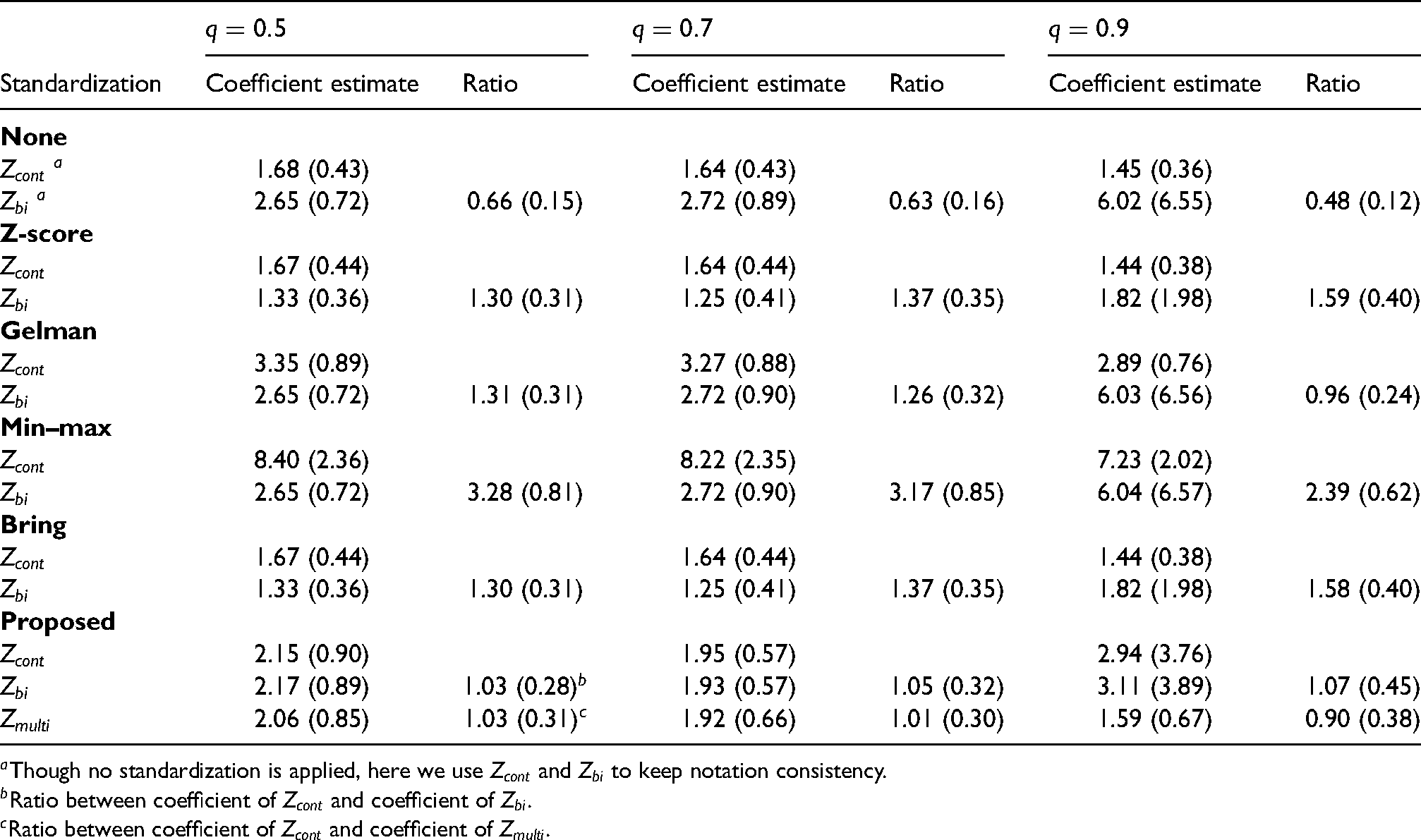
We expect the appropriately standardized coefficients of $Z_{c o n t}$ , $Z_{b i}$ and $Z_{m u l t i}$ from the logistic regression to be equal because the original impacts of the latent covariates $X_{1}$ , $X_{2}$ and $X_{3}$ are equal. That is, the closer the ratios to one the better the standardization reflects the covariates’ relative impacts. As can be observed from Table 1, without standardization, binary covariates have larger coefficient values and also larger standard deviations. The difference between coefficients of $Z_{c o n t}$ and $Z_{b i}$ gets bigger when $q$ , the probability of the observed binary covariate, gets more extreme. On the contrary, Min–max standardization leads to much larger coefficients for $Z_{c o n t}$ than $Z_{b i}$ . Z-score standardization makes the coefficients of standardized continuous and binary covariates much closer but still favors the continuous covariates with slightly larger coefficients when binary covariate probability is not extreme. Not surprisingly, Bring standardization has the same result as Z-score, since in the simulation setup, $X_{c o n t}$ and $X_{b i}$ are independent, so Bring and Z-score are equivalent. Gelman standardization also makes the coefficients of $Z_{c o n t}$ and $Z_{b i}$ closer, similar to the result of Z-score and Bring standardization methods. In summary, the proposed standardization is the most successful in getting equal coefficient values for standardized continuous, binary and multi-level covariates. When examining the coefficient relation by ratios, no standardization and Min–Max standardization make the coefficient ratios far away from one. The other four standardization approaches keep the ratios closer to one but the proposed method gives the ratios closest to one, which implies that the proposed standardization is able to recover covariates relative impacts regardless of their types, and this corroborates the statement in Lemma 1. The slight deviation from one is likely due to the small sample size ( $n = 100$ ) in the simulation, a conservative yet realistic setup.
3.2. Simulation II: select covariates fairly with standardization

	$q = 0.5$	$q = 0.7$	$q = 0.9$
None
$Z_{c o n t}$ $^{a}$	1.68 (0.43)		1.64 (0.43)		1.45 (0.36)
$Z_{b i}$ $^{a}$	2.65 (0.72)	0.66 (0.15)	2.72 (0.89)	0.63 (0.16)	6.02 (6.55)	0.48 (0.12)
Z-score
$Z_{c o n t}$	1.67 (0.44)		1.64 (0.44)		1.44 (0.38)
$Z_{b i}$	1.33 (0.36)	1.30 (0.31)	1.25 (0.41)	1.37 (0.35)	1.82 (1.98)	1.59 (0.40)
Gelman
$Z_{c o n t}$	3.35 (0.89)		3.27 (0.88)		2.89 (0.76)
$Z_{b i}$	2.65 (0.72)	1.31 (0.31)	2.72 (0.90)	1.26 (0.32)	6.03 (6.56)	0.96 (0.24)
Min–max
$Z_{c o n t}$	8.40 (2.36)		8.22 (2.35)		7.23 (2.02)
$Z_{b i}$	2.65 (0.72)	3.28 (0.81)	2.72 (0.90)	3.17 (0.85)	6.04 (6.57)	2.39 (0.62)
Bring
$Z_{c o n t}$	1.67 (0.44)		1.64 (0.44)		1.44 (0.38)
$Z_{b i}$	1.33 (0.36)	1.30 (0.31)	1.25 (0.41)	1.37 (0.35)	1.82 (1.98)	1.58 (0.40)
Proposed
$Z_{c o n t}$	2.15 (0.90)		1.95 (0.57)		2.94 (3.76)
$Z_{b i}$	2.17 (0.89)	1.03 (0.28) $^{b}$	1.93 (0.57)	1.05 (0.32)	3.11 (3.89)	1.07 (0.45)
$Z_{m u l t i}$	2.06 (0.85)	1.03 (0.31) $^{c}$	1.92 (0.66)	1.01 (0.30)	1.59 (0.67)	0.90 (0.38)

In simulation II, for each standardization method, we examine how the capacity of recovering covariate impacts affects the selection probabilities of covariates of different types in the sparse penalized regressions. In the simulation outcome generation model, there are 12 latent continuous covariates in total. The first six are important covariates assigned with nonzero and equal coefficient size (i.e. equal impact), and the last six are noise covariates assigned with zero coefficient size. Next we transform latent variables to observed covariates in different types (i.e. continuous, binary and categorical). Then we perform group-lasso logistic regression on the standardized versions of the observed data. We expect that a good standardization method would lead to comparable selection probabilities for covariates with equal impacts.

The simulation setup is as follows.

Generate 12 latent continuous variables $X_{n \times m} = (X_{1}, \dots, X_{6}, X_{7}, \dots, X_{12})$ from multivariate normal distribution $N (0_{m \times 1}, I_{m \times m})$ , where $I$ is identity matrix, $n = 200$ and $m = 12$ .

Generate the binary outcome $Y$ by sampling from Bernoulli distribution with probability $\frac{\exp {η_{i}}}{1 + \exp {η_{i}}}$ , where $η_{i} = 2 X_{i 1} + 2 X_{i 2} + 2 X_{i 3} - 2 X_{i 4} - 2 X_{i 5} - 2 X_{i 6}^{2}$ , $i = 1, \dots, n$ . The first six are true covariates with coefficient sizes equal to two, and the last six are noise covariates with coefficients equal to zero. Moreover, we assume $X_{6}$ and $X_{12}$ have quadratic relationships with the outcome.

Generate the observed covariates:

c.1
$X 1_{c o n t} = X_{1}$ , $X 7_{c o n t} = X_{7}$ ;
c.2
$X 2_{b i_p 0.5} = I (X_{2} < Φ^{- 1} (0.5))$ , $X 8_{b i_p 0.5} = I (X_{8} < Φ^{- 1} (0.5))$ ;
c.3
$X 3_{b i_p 0.7} = I (X_{3} < Φ^{- 1} (0.7))$ , $X 9_{b i_p 0.7} = I (X_{9} < Φ^{- 1} (0.7))$ ;
c.4
$X 4_{b i_p 0.9} = I (X_{4} < Φ^{- 1} (0.9))$ , $X 10_{b i_p 0.9} = I (X_{10} < Φ^{- 1} (0.9))$ ;
c.5
$X 5_{m u l t i 3} = I (Φ^{- 1} (\frac{1}{3}) < X_{5} \leq Φ^{- 1} (\frac{2}{3})) + 2 \times I (Φ^{- 1} (\frac{2}{3}) < X_{5})$ ,

$X 11_{m u l t i 3} = I (Φ^{- 1} (\frac{1}{3}) < X_{11} \leq Φ^{- 1} (\frac{2}{3})) + 2 \times I (Φ^{- 1} (\frac{2}{3}) < X_{11})$ ;
c.6
$X 6_{c o n t} = X_{6}, X 12_{c o n t} = X_{12}$ .
In summary, $X 1_{c o n t}$ and $X 7_{c o n t}$ are continuous; $X 6_{c o n t}$ and $X 12_{c o n t}$ are continuous; $X 2_{b i_p 0.5}$ and $X 8_{b i_p 0.5}$ , $X 3_{b i_p 0.7}$ and $X 9_{b i_p 0.7}$ , $X 4_{b i_p 0.9}$ and $X 10_{b i_p 0.9}$ are binary variables with probabilities equal to 0.5, 0.7 and 0.9 respectively; $X 5_{m u l t i 3}$ and $X 11_{m u l t i 3}$ are multi-category variables taking values in {0,1,2}.

Standardize the observed data $(X 1_{c o n t}, \dots, X 6_{c o n t}, X 7_{c o n t}, \dots, X 12_{c o n t})$ to $(Z 1_{c o n t}, \dots, Z 6_{c o n t}, Z 7_{c o n t}, \dots, Z 12_{c o n t})$ using different methods, then fit group-lasso logistic regression of $Y$ on $(Z 1_{c o n t}, \dots, Z 12_{c o n t}^{2})$ and record the selected covariates. Specifically, we standardize the quadratic covariates $X 6_{c o n t}^{2}$ and $X 12_{c o n t}^{2}$ using the standard deviation of $X 6_{c o n t}$ and $X 12_{c o n t}$ when implementing the Z-score, Gelman, and Bring standardization, since we are interested in the impacts with changes in $X 6_{c o n t}$ and $X 12_{c o n t}$ . And we standardize $X 6_{c o n t}^{2}$ and $X 12_{c o n t}^{2}$ using the range or percentile of $X 6_{c o n t}^{2}$ and $X 12_{c o n t}^{2}$ when performing the Min–max and the proposed standardization, because these two standardization methods concern the range of the covariate impacts on the outcome.
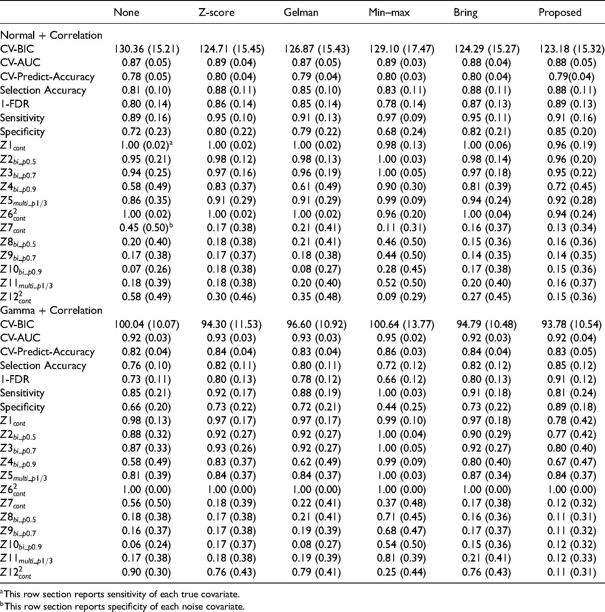
We experiment the simulation setup with two latent distributions, symmetric normal distribution and skewed gamma distribution (shape = 2, scale = 2) , in order to examine how the distribution skewness affects the standardization performance. Additionally, with both distributions, we also inspect the situation where latent variables are correlated with correlation equal to 0.1. Under each scenario, the above simulation setup is repeated 2000 times, and the results are reported in Tables 2 and 3. One thing worth noting is that when applying the proposed standardization, by the criterion described in Section 2.2., we set the cutoff $100 p$ -th percentile with $p = 0.5$ because the observed binary variables have probabilities from 0.5 to 0.9. That is, we dichotomize continuous variables $X 1_{c o n t}, X 6_{c o n t}^{2}, X 7_{c o n t}, X 12_{c o n t}^{2}$ by their $50$ -th percentiles, and regroup multi-category variables $X 5_{m u l t i 3}$ , $X 11_{m u l t i 3}$ to binary variables of probabilities closest to 0.5.

Table 2.
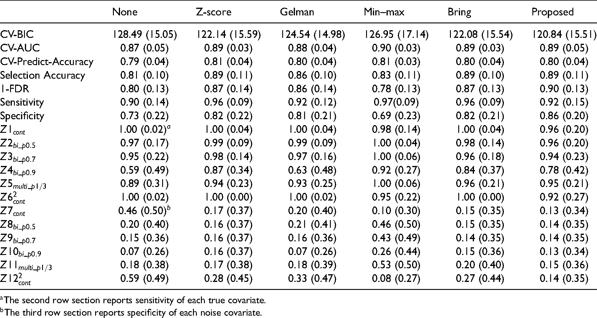
Performance of variable selection using different standardization methods when effects/associations are of the same size (coefficient size of the latent continuous covariates is two for Z1 to Z6 and coefficient size of the latent continuous covariates is zero for Z7 to Z12)

None Z-score Gelman Min–max Bring Proposed

CV-BIC 128.49 (15.05) 122.14 (15.59) 124.54 (14.98) 126.95 (17.14) 122.08 (15.54) 120.84 (15.51)

CV-AUC 0.87 (0.05) 0.89 (0.03) 0.88 (0.04) 0.90 (0.03) 0.89 (0.03) 0.89 (0.05)

CV-Predict-Accuracy 0.79 (0.04) 0.81 (0.04) 0.80 (0.04) 0.81 (0.03) 0.80 (0.04) 0.80 (0.04)

Selection Accuracy 0.81 (0.10) 0.89 (0.11) 0.86 (0.10) 0.83 (0.11) 0.89 (0.10) 0.89 (0.11)

1-FDR 0.80 (0.13) 0.87 (0.14) 0.86 (0.14) 0.78 (0.13) 0.87 (0.13) 0.90 (0.13)

Sensitivity 0.90 (0.14) 0.96 (0.09) 0.92 (0.12) 0.97(0.09) 0.96 (0.09) 0.92 (0.15)

Specificity 0.73 (0.22) 0.82 (0.22) 0.81 (0.21) 0.69 (0.23) 0.82 (0.21) 0.86 (0.20)

$Z 1_{c o n t}$ 1.00 (0.02) $^{a}$ 1.00 (0.04) 1.00 (0.04) 0.98 (0.14) 1.00 (0.04) 0.96 (0.20)

$Z 2_{b i_p 0.5}$ 0.97 (0.17) 0.99 (0.09) 0.99 (0.09) 1.00 (0.04) 0.98 (0.14) 0.96 (0.20)

$Z 3_{b i_p 0.7}$ 0.95 (0.22) 0.98 (0.14) 0.97 (0.16) 1.00 (0.06) 0.96 (0.18) 0.94 (0.23)

$Z 4_{b i_p 0.9}$ 0.59 (0.49) 0.87 (0.34) 0.63 (0.48) 0.92 (0.27) 0.84 (0.37) 0.78 (0.42)

$Z 5_{m u l t i_p 1 / 3}$ 0.89 (0.31) 0.94 (0.23) 0.93 (0.25) 1.00 (0.06) 0.96 (0.21) 0.95 (0.21)

$Z 6_{c o n t}^{2}$ 1.00 (0.02) 1.00 (0.00) 1.00 (0.02) 0.95 (0.22) 1.00 (0.00) 0.92 (0.27)

$Z 7_{c o n t}$ 0.46 (0.50) $^{b}$ 0.17 (0.37) 0.20 (0.40) 0.10 (0.30) 0.15 (0.35) 0.13 (0.34)

$Z 8_{b i_p 0.5}$ 0.20 (0.40) 0.16 (0.37) 0.21 (0.41) 0.46 (0.50) 0.15 (0.35) 0.14 (0.35)

$Z 9_{b i_p 0.7}$ 0.15 (0.36) 0.16 (0.37) 0.16 (0.36) 0.43 (0.49) 0.14 (0.35) 0.14 (0.35)

$Z 10_{b i_p 0.9}$ 0.07 (0.26) 0.16 (0.37) 0.07 (0.26) 0.26 (0.44) 0.15 (0.36) 0.13 (0.34)

$Z 11_{m u l t i_p 1 / 3}$ 0.18 (0.38) 0.17 (0.38) 0.18 (0.39) 0.53 (0.50) 0.20 (0.40) 0.15 (0.36)

$Z 12_{c o n t}^{2}$ 0.59 (0.49) 0.28 (0.45) 0.33 (0.47) 0.08 (0.27) 0.27 (0.44) 0.14 (0.35)

$^{a}$ The second row section reports sensitivity of each true covariate.

$^{b}$ The third row section reports specificity of each noise covariate.

Table 3.
Performance of variable selection using different standardization methods in the presence of correlated covariates (the correlations between the latent covariates are 0.1)

None Z-score Gelman Min–max Bring Proposed

Normal + Correlation

CV-BIC 130.36 (15.21) 124.71 (15.45) 126.87 (15.43) 129.10 (17.47) 124.29 (15.27) 123.18 (15.32)

CV-AUC 0.87 (0.05) 0.89 (0.04) 0.87 (0.05) 0.89 (0.03) 0.88 (0.04) 0.88 (0.05)

CV-Predict-Accuracy 0.78 (0.05) 0.80 (0.04) 0.79 (0.04) 0.80 (0.03) 0.80 (0.04) 0.79(0.04)

Selection Accuracy 0.81 (0.10) 0.88 (0.11) 0.85 (0.10) 0.83 (0.11) 0.88 (0.11) 0.88 (0.11)

1-FDR 0.80 (0.14) 0.86 (0.14) 0.85 (0.14) 0.78 (0.14) 0.87 (0.13) 0.89 (0.13)

Sensitivity 0.89 (0.16) 0.95 (0.10) 0.91 (0.13) 0.97 (0.09) 0.95 (0.11) 0.91 (0.16)

Specificity 0.72 (0.23) 0.80 (0.22) 0.79 (0.22) 0.68 (0.24) 0.82 (0.21) 0.85 (0.20)

$Z 1_{c o n t}$ 1.00 (0.02) $^{a}$ 1.00 (0.02) 1.00 (0.02) 0.98 (0.13) 1.00 (0.06) 0.96 (0.19)

$Z 2_{b i_p 0.5}$ 0.95 (0.21) 0.98 (0.12) 0.98 (0.13) 1.00 (0.03) 0.98 (0.14) 0.96 (0.20)

$Z 3_{b i_p 0.7}$ 0.94 (0.25) 0.97 (0.16) 0.96 (0.19) 1.00 (0.05) 0.97 (0.18) 0.95 (0.22)

$Z 4_{b i_p 0.9}$ 0.58 (0.49) 0.83 (0.37) 0.61 (0.49) 0.90 (0.30) 0.81 (0.39) 0.72 (0.45)

$Z 5_{m u l t i_p 1 / 3}$ 0.86 (0.35) 0.91 (0.29) 0.91 (0.29) 0.99 (0.09) 0.94 (0.24) 0.92 (0.28)

$Z 6_{c o n t}^{2}$ 1.00 (0.02) 1.00 (0.02) 1.00 (0.02) 0.96 (0.20) 1.00 (0.04) 0.94 (0.24)

$Z 7_{c o n t}$ 0.45 (0.50) $^{b}$ 0.17 (0.38) 0.21 (0.41) 0.11 (0.31) 0.16 (0.37) 0.13 (0.34)

$Z 8_{b i_p 0.5}$ 0.20 (0.40) 0.18 (0.38) 0.21 (0.41) 0.46 (0.50) 0.15 (0.36) 0.16 (0.36)

$Z 9_{b i_p 0.7}$ 0.17 (0.38) 0.17 (0.37) 0.18 (0.38) 0.44 (0.50) 0.14 (0.35) 0.14 (0.35)

$Z 10_{b i_p 0.9}$ 0.07 (0.26) 0.18 (0.38) 0.08 (0.27) 0.28 (0.45) 0.17 (0.38) 0.15 (0.36)

$Z 11_{m u l t i_p 1 / 3}$ 0.18 (0.39) 0.18 (0.38) 0.20 (0.40) 0.52 (0.50) 0.20 (0.40) 0.16 (0.37)

$Z 12_{c o n t}^{2}$ 0.58 (0.49) 0.30 (0.46) 0.35 (0.48) 0.09 (0.29) 0.27 (0.45) 0.15 (0.36)

Gamma + Correlation

CV-BIC 100.04 (10.07) 94.30 (11.53) 96.60 (10.92) 100.64 (13.77) 94.79 (10.48) 93.78 (10.54)

CV-AUC 0.92 (0.03) 0.93 (0.03) 0.93 (0.03) 0.95 (0.02) 0.92 (0.03) 0.92 (0.04)

CV-Predict-Accuracy 0.82 (0.04) 0.84 (0.04) 0.83 (0.04) 0.86 (0.03) 0.84 (0.04) 0.83 (0.05)

Selection Accuracy 0.76 (0.10) 0.82 (0.11) 0.80 (0.11) 0.72 (0.12) 0.82 (0.12) 0.85 (0.12)

1-FDR 0.73 (0.11) 0.80 (0.13) 0.78 (0.12) 0.66 (0.12) 0.80 (0.13) 0.91 (0.12)

Sensitivity 0.85 (0.21) 0.92 (0.17) 0.88 (0.19) 1.00 (0.03) 0.91 (0.18) 0.81 (0.24)

Specificity 0.66 (0.20) 0.73 (0.22) 0.72 (0.21) 0.44 (0.25) 0.73 (0.22) 0.89 (0.18)

$Z 1_{c o n t}$ 0.98 (0.13) 0.97 (0.17) 0.97 (0.17) 0.99 (0.10) 0.97 (0.18) 0.78 (0.42)

$Z 2_{b i_p 0.5}$ 0.88 (0.32) 0.92 (0.27) 0.92 (0.27) 1.00 (0.04) 0.90 (0.29) 0.77 (0.42)

$Z 3_{b i_p 0.7}$ 0.87 (0.33) 0.93 (0.26) 0.92 (0.27) 1.00 (0.05) 0.92 (0.27) 0.80 (0.40)

$Z 4_{b i_p 0.9}$ 0.58 (0.49) 0.83 (0.37) 0.62 (0.49) 0.99 (0.09) 0.80 (0.40) 0.67 (0.47)

$Z 5_{m u l t i_p 1 / 3}$ 0.81 (0.39) 0.84 (0.37) 0.84 (0.37) 1.00 (0.03) 0.87 (0.34) 0.84 (0.37)

$Z 6_{c o n t}^{2}$ 1.00 (0.00) 1.00 (0.00) 1.00 (0.00) 1.00 (0.00) 1.00 (0.00) 1.00 (0.00)

$Z 7_{c o n t}$ 0.56 (0.50) 0.18 (0.39) 0.22 (0.41) 0.37 (0.48) 0.17 (0.38) 0.12 (0.32)

$Z 8_{b i_p 0.5}$ 0.18 (0.38) 0.17 (0.38) 0.21 (0.41) 0.71 (0.45) 0.16 (0.36) 0.11 (0.31)

$Z 9_{b i_p 0.7}$ 0.16 (0.37) 0.17 (0.38) 0.19 (0.39) 0.68 (0.47) 0.17 (0.37) 0.11 (0.32)

$Z 10_{b i_p 0.9}$ 0.06 (0.24) 0.17 (0.37) 0.08 (0.27) 0.54 (0.50) 0.15 (0.36) 0.12 (0.32)

$Z 11_{m u l t i_p 1 / 3}$ 0.17 (0.38) 0.18 (0.38) 0.19 (0.39) 0.81 (0.39) 0.21 (0.41) 0.12 (0.33)

$Z 12_{c o n t}^{2}$ 0.90 (0.30) 0.76 (0.43) 0.79 (0.41) 0.25 (0.44) 0.76 (0.43) 0.11 (0.31)

$^{a}$ This row section reports sensitivity of each true covariate.

$^{b}$ This row section reports specificity of each noise covariate.

In Tables 2 and 3, the columns display the results of different standardization methods. When conducting the group-lasso regression, the default sequence of candidate penalty $λ$ provided by the gglasso R package is used, and the $λ$ with the cross-validation misclassification error one standard deviation larger than the minimum cross-validation misclassification error is employed as the regularization value to select the covariates. Then we calculate the sensitivity (percent of true variables being selected of all the true variables), specificity (percent of noise variables not being selected of all the noise variables), selection accuracy (average of sensitivity and specificity), and 1-FDR (percent of true variables being selected of all the selected variables). In addition, we use 2-fold cross-validation (CV) to evaluate the performance of the logistic regression model fitted with the selected variables with respect to Bayesian information criterion (BIC), area under the receiver operating characteristic curve (AUC), and prediction accuracy (percent of predicted outcome being consistent with the true outcome). The averages of those performance measurements are recorded in the top section of the tables. The second and third sections report the average sensitivity or specificity of each individual covariate, with the empirical standard deviation in the parenthesis. In Tables 2 and 3, the proposed method has the best performance in terms of lower CV-BIC, higher selection accuracy, higher 1-FDR and higher specificity in all six methods.

There are some patterns observed from Table 2. Without any standardization, the continuous variables are favored with higher selection rates, regardless the relationship being linear or quadratic, compared to binary and multi-category variables. Among the categorical covariates, binary variables of probability 0.5 or 0.7 have higher selection rates than multi-category covariates. The selection rate decreases when the probability of binary variable gets more extreme. Similar behaviors are also observed when using Z-score, Gelman and Bring standardization approaches. Notice that the aforementioned four standardization methods do not eliminate the essential difference between a variable being continuous and a variable being binary, so those detected patterns are likely due to Lasso’s beta-min condition,⁷ which establishes a lower bound for the amount of signal, such as signal-to-noise ratio (SNR), required for feature recovery. As a result, Gaussian variables have a higher probability of being selected than binary variables because they demand lower thresholds. Meanwhile, binary variables with more extreme probabilities require higher signal thresholds, therefore are less likely to be selected. Although Min-Max standardization produces large coefficient estimates for continuous covariates (from simulation I), the continuous variable is disfavored with smaller selection rate compared with the binary and multi-category variables. Above all, the proposed standardization produces similar selection rates across covariates of different types, though the selection rate of binary covariate still goes down with extreme probability 0.9. Since the proposed standardization actually convert observed covariates of different types into binary variables of similar probabilities, according to Lasso’s beta-min condition, they have similar signal thresholds. The simulation result of the proposed method corroborates the statement in Lemma 2.

Table 3 displays the simulation results of different latent distributions with correlation structures. According to the irrepresentable theorem,¹⁷ the selection consistency would be compromised if the true covariates are highly correlated with the noise variables, and we do observe that performance measurements, especially the overall sensitivity, in Table 3 are worse than those reported in Table 2. In spite of the correlation structure, patterns observed in Table 2 still apply to data in Table 3.
4. Real data example

	None	Z-score	Gelman	Min–max	Bring	Proposed
CV-BIC	128.49 (15.05)	122.14 (15.59)	124.54 (14.98)	126.95 (17.14)	122.08 (15.54)	120.84 (15.51)
CV-AUC	0.87 (0.05)	0.89 (0.03)	0.88 (0.04)	0.90 (0.03)	0.89 (0.03)	0.89 (0.05)
CV-Predict-Accuracy	0.79 (0.04)	0.81 (0.04)	0.80 (0.04)	0.81 (0.03)	0.80 (0.04)	0.80 (0.04)
Selection Accuracy	0.81 (0.10)	0.89 (0.11)	0.86 (0.10)	0.83 (0.11)	0.89 (0.10)	0.89 (0.11)
1-FDR	0.80 (0.13)	0.87 (0.14)	0.86 (0.14)	0.78 (0.13)	0.87 (0.13)	0.90 (0.13)
Sensitivity	0.90 (0.14)	0.96 (0.09)	0.92 (0.12)	0.97(0.09)	0.96 (0.09)	0.92 (0.15)
Specificity	0.73 (0.22)	0.82 (0.22)	0.81 (0.21)	0.69 (0.23)	0.82 (0.21)	0.86 (0.20)
$Z 1_{c o n t}$	1.00 (0.02) $^{a}$	1.00 (0.04)	1.00 (0.04)	0.98 (0.14)	1.00 (0.04)	0.96 (0.20)
$Z 2_{b i_p 0.5}$	0.97 (0.17)	0.99 (0.09)	0.99 (0.09)	1.00 (0.04)	0.98 (0.14)	0.96 (0.20)
$Z 3_{b i_p 0.7}$	0.95 (0.22)	0.98 (0.14)	0.97 (0.16)	1.00 (0.06)	0.96 (0.18)	0.94 (0.23)
$Z 4_{b i_p 0.9}$	0.59 (0.49)	0.87 (0.34)	0.63 (0.48)	0.92 (0.27)	0.84 (0.37)	0.78 (0.42)
$Z 5_{m u l t i_p 1 / 3}$	0.89 (0.31)	0.94 (0.23)	0.93 (0.25)	1.00 (0.06)	0.96 (0.21)	0.95 (0.21)
$Z 6_{c o n t}^{2}$	1.00 (0.02)	1.00 (0.00)	1.00 (0.02)	0.95 (0.22)	1.00 (0.00)	0.92 (0.27)
$Z 7_{c o n t}$	0.46 (0.50) $^{b}$	0.17 (0.37)	0.20 (0.40)	0.10 (0.30)	0.15 (0.35)	0.13 (0.34)
$Z 8_{b i_p 0.5}$	0.20 (0.40)	0.16 (0.37)	0.21 (0.41)	0.46 (0.50)	0.15 (0.35)	0.14 (0.35)
$Z 9_{b i_p 0.7}$	0.15 (0.36)	0.16 (0.37)	0.16 (0.36)	0.43 (0.49)	0.14 (0.35)	0.14 (0.35)
$Z 10_{b i_p 0.9}$	0.07 (0.26)	0.16 (0.37)	0.07 (0.26)	0.26 (0.44)	0.15 (0.36)	0.13 (0.34)
$Z 11_{m u l t i_p 1 / 3}$	0.18 (0.38)	0.17 (0.38)	0.18 (0.39)	0.53 (0.50)	0.20 (0.40)	0.15 (0.36)
$Z 12_{c o n t}^{2}$	0.59 (0.49)	0.28 (0.45)	0.33 (0.47)	0.08 (0.27)	0.27 (0.44)	0.14 (0.35)

	None	Z-score	Gelman	Min–max	Bring	Proposed
Normal + Correlation
CV-BIC	130.36 (15.21)	124.71 (15.45)	126.87 (15.43)	129.10 (17.47)	124.29 (15.27)	123.18 (15.32)
CV-AUC	0.87 (0.05)	0.89 (0.04)	0.87 (0.05)	0.89 (0.03)	0.88 (0.04)	0.88 (0.05)
CV-Predict-Accuracy	0.78 (0.05)	0.80 (0.04)	0.79 (0.04)	0.80 (0.03)	0.80 (0.04)	0.79(0.04)
Selection Accuracy	0.81 (0.10)	0.88 (0.11)	0.85 (0.10)	0.83 (0.11)	0.88 (0.11)	0.88 (0.11)
1-FDR	0.80 (0.14)	0.86 (0.14)	0.85 (0.14)	0.78 (0.14)	0.87 (0.13)	0.89 (0.13)
Sensitivity	0.89 (0.16)	0.95 (0.10)	0.91 (0.13)	0.97 (0.09)	0.95 (0.11)	0.91 (0.16)
Specificity	0.72 (0.23)	0.80 (0.22)	0.79 (0.22)	0.68 (0.24)	0.82 (0.21)	0.85 (0.20)
$Z 1_{c o n t}$	1.00 (0.02) $^{a}$	1.00 (0.02)	1.00 (0.02)	0.98 (0.13)	1.00 (0.06)	0.96 (0.19)
$Z 2_{b i_p 0.5}$	0.95 (0.21)	0.98 (0.12)	0.98 (0.13)	1.00 (0.03)	0.98 (0.14)	0.96 (0.20)
$Z 3_{b i_p 0.7}$	0.94 (0.25)	0.97 (0.16)	0.96 (0.19)	1.00 (0.05)	0.97 (0.18)	0.95 (0.22)
$Z 4_{b i_p 0.9}$	0.58 (0.49)	0.83 (0.37)	0.61 (0.49)	0.90 (0.30)	0.81 (0.39)	0.72 (0.45)
$Z 5_{m u l t i_p 1 / 3}$	0.86 (0.35)	0.91 (0.29)	0.91 (0.29)	0.99 (0.09)	0.94 (0.24)	0.92 (0.28)
$Z 6_{c o n t}^{2}$	1.00 (0.02)	1.00 (0.02)	1.00 (0.02)	0.96 (0.20)	1.00 (0.04)	0.94 (0.24)
$Z 7_{c o n t}$	0.45 (0.50) $^{b}$	0.17 (0.38)	0.21 (0.41)	0.11 (0.31)	0.16 (0.37)	0.13 (0.34)
$Z 8_{b i_p 0.5}$	0.20 (0.40)	0.18 (0.38)	0.21 (0.41)	0.46 (0.50)	0.15 (0.36)	0.16 (0.36)
$Z 9_{b i_p 0.7}$	0.17 (0.38)	0.17 (0.37)	0.18 (0.38)	0.44 (0.50)	0.14 (0.35)	0.14 (0.35)
$Z 10_{b i_p 0.9}$	0.07 (0.26)	0.18 (0.38)	0.08 (0.27)	0.28 (0.45)	0.17 (0.38)	0.15 (0.36)
$Z 11_{m u l t i_p 1 / 3}$	0.18 (0.39)	0.18 (0.38)	0.20 (0.40)	0.52 (0.50)	0.20 (0.40)	0.16 (0.37)
$Z 12_{c o n t}^{2}$	0.58 (0.49)	0.30 (0.46)	0.35 (0.48)	0.09 (0.29)	0.27 (0.45)	0.15 (0.36)
Gamma + Correlation
CV-BIC	100.04 (10.07)	94.30 (11.53)	96.60 (10.92)	100.64 (13.77)	94.79 (10.48)	93.78 (10.54)
CV-AUC	0.92 (0.03)	0.93 (0.03)	0.93 (0.03)	0.95 (0.02)	0.92 (0.03)	0.92 (0.04)
CV-Predict-Accuracy	0.82 (0.04)	0.84 (0.04)	0.83 (0.04)	0.86 (0.03)	0.84 (0.04)	0.83 (0.05)
Selection Accuracy	0.76 (0.10)	0.82 (0.11)	0.80 (0.11)	0.72 (0.12)	0.82 (0.12)	0.85 (0.12)
1-FDR	0.73 (0.11)	0.80 (0.13)	0.78 (0.12)	0.66 (0.12)	0.80 (0.13)	0.91 (0.12)
Sensitivity	0.85 (0.21)	0.92 (0.17)	0.88 (0.19)	1.00 (0.03)	0.91 (0.18)	0.81 (0.24)
Specificity	0.66 (0.20)	0.73 (0.22)	0.72 (0.21)	0.44 (0.25)	0.73 (0.22)	0.89 (0.18)
$Z 1_{c o n t}$	0.98 (0.13)	0.97 (0.17)	0.97 (0.17)	0.99 (0.10)	0.97 (0.18)	0.78 (0.42)
$Z 2_{b i_p 0.5}$	0.88 (0.32)	0.92 (0.27)	0.92 (0.27)	1.00 (0.04)	0.90 (0.29)	0.77 (0.42)
$Z 3_{b i_p 0.7}$	0.87 (0.33)	0.93 (0.26)	0.92 (0.27)	1.00 (0.05)	0.92 (0.27)	0.80 (0.40)
$Z 4_{b i_p 0.9}$	0.58 (0.49)	0.83 (0.37)	0.62 (0.49)	0.99 (0.09)	0.80 (0.40)	0.67 (0.47)
$Z 5_{m u l t i_p 1 / 3}$	0.81 (0.39)	0.84 (0.37)	0.84 (0.37)	1.00 (0.03)	0.87 (0.34)	0.84 (0.37)
$Z 6_{c o n t}^{2}$	1.00 (0.00)	1.00 (0.00)	1.00 (0.00)	1.00 (0.00)	1.00 (0.00)	1.00 (0.00)
$Z 7_{c o n t}$	0.56 (0.50)	0.18 (0.39)	0.22 (0.41)	0.37 (0.48)	0.17 (0.38)	0.12 (0.32)
$Z 8_{b i_p 0.5}$	0.18 (0.38)	0.17 (0.38)	0.21 (0.41)	0.71 (0.45)	0.16 (0.36)	0.11 (0.31)
$Z 9_{b i_p 0.7}$	0.16 (0.37)	0.17 (0.38)	0.19 (0.39)	0.68 (0.47)	0.17 (0.37)	0.11 (0.32)
$Z 10_{b i_p 0.9}$	0.06 (0.24)	0.17 (0.37)	0.08 (0.27)	0.54 (0.50)	0.15 (0.36)	0.12 (0.32)
$Z 11_{m u l t i_p 1 / 3}$	0.17 (0.38)	0.18 (0.38)	0.19 (0.39)	0.81 (0.39)	0.21 (0.41)	0.12 (0.33)
$Z 12_{c o n t}^{2}$	0.90 (0.30)	0.76 (0.43)	0.79 (0.41)	0.25 (0.44)	0.76 (0.43)	0.11 (0.31)

Opioid abuse has been the number one reason of death due to drug overdose in the US. According to the Center for Disease Control (CDC),¹⁸ nearly 70% of the drug overdose deaths in 2018 involved an opioid, and 32% of those opioid overdose deaths was attributable to prescription opioid. In the 12-month period that ended in April 2021,¹⁹ the overdose death toll reached a record high number in the US, more than 100,000 Americans died of overdoses, more than the toll of car crashes and gun fatalities combined. Thus, it is of great importance to study the pattern and identify the factors associated with opioid prescription, which would further serve as evidences to inform and reinforce interventions seeking to reduce unnecessary opioid prescriptions. The National Ambulatory Medical Care Survey (NAMCS) is jointly conducted by the CDC and the National Center of Health Statistics yearly since 1973, it examines office visits from a sample of office-based physicians across the US. The data includes visits information, prescription medications, patient and physician characteristics. We apply penalized logistic regression model on the NAMCS data to explore factors related to opioid prescription in US, as well as illustrate and compare the performance of all six standardization methods (None, Z-score, Gelman, Min–max, Bring, and Proposed).

In total 10,031 observations (rows) and 177 input variables (columns) are used in the final analysis. Among the 177 input features, three of them are continuous, 139 are binary and 35 are the multi-category type. More than three-fourths of the binary variables have empirical probabilities greater than 0.9 or less than 0.1, and most of the multi-category variables have categories with frequencies less than 0.1. The outcome variable is a binary variable with a value one indicating opioid prescription, and zero otherwise. In addition, each observation has a sampling weight calculated as the product of the patient level weight and the physician level weight that produces nationally representative estimates. We notice that in the real data, (1) there are three data types and the majority are binary and categorical variables; (2) extreme frequencies of categories, such as 0.9 or 0.1, prevail in the binary and categorical variables. Those observations will later be used to justify the choice of the $90$ -th percentile as cutoff in the proposed standardization.

Weighted group-lasso logistic regression is conducted on the standardized NAMCS data using different standardization methods, the performance is summarized in Figure 1 and Table 4. For each standardization approach, (1) we first construct a sequence of penalty $λ$ values of size 125, $Λ = {λ_{1}, \dots, λ_{125}}$ (the same sequence is shared by all standardization methods); (2) then fit the weighted group-lasso logistic regression on the standardized data using each $λ$ from $Λ$ and record the corresponding selected variables, which gives $S = {S_{1}, \dots, S_{125}}$ , where $S_{i}$ is the set of covariates selected by the penalized model using penalty $λ_{i}$ ; (3) refit a logistic regression using the original forms of the selected variables in $S_{i}$ and calculate the corresponding BIC $_{i}$ , AUC $_{i}$ and log-likelihood; (4) identify the BIC $_{1 s e}$ value that is one standard deviation larger than the minimum BIC, then locate the $λ_{B I C_{1 s e}}$ that corresponds to the BIC $_{1 s e}$ . When applying the proposed method, since the majority of the binary variables have empirical probabilities greater than 0.9 or less than 0.1, we set $p = 0.9$ . That is, we dichotomize the continuous variable by its $90$ -th percentile, and regroup the multi-category variable to binary with the percentage of ones of the newly constructed binary as close to 0.9 as possible. We have also experimented with $p = 0.5$ and $p = 0.7$ , which produces similar results. When $p = 0.5$ , BIC $=$ 85120.22 and AUC $=$ 0.84; When $p = 0.7$ , BIC $=$ 85631.91 and AUC $=$ 0.84, compared with when $p = 0.9$ , BIC $=$ 85290.75, and AUC $=$ 0.84.

Figure 1.

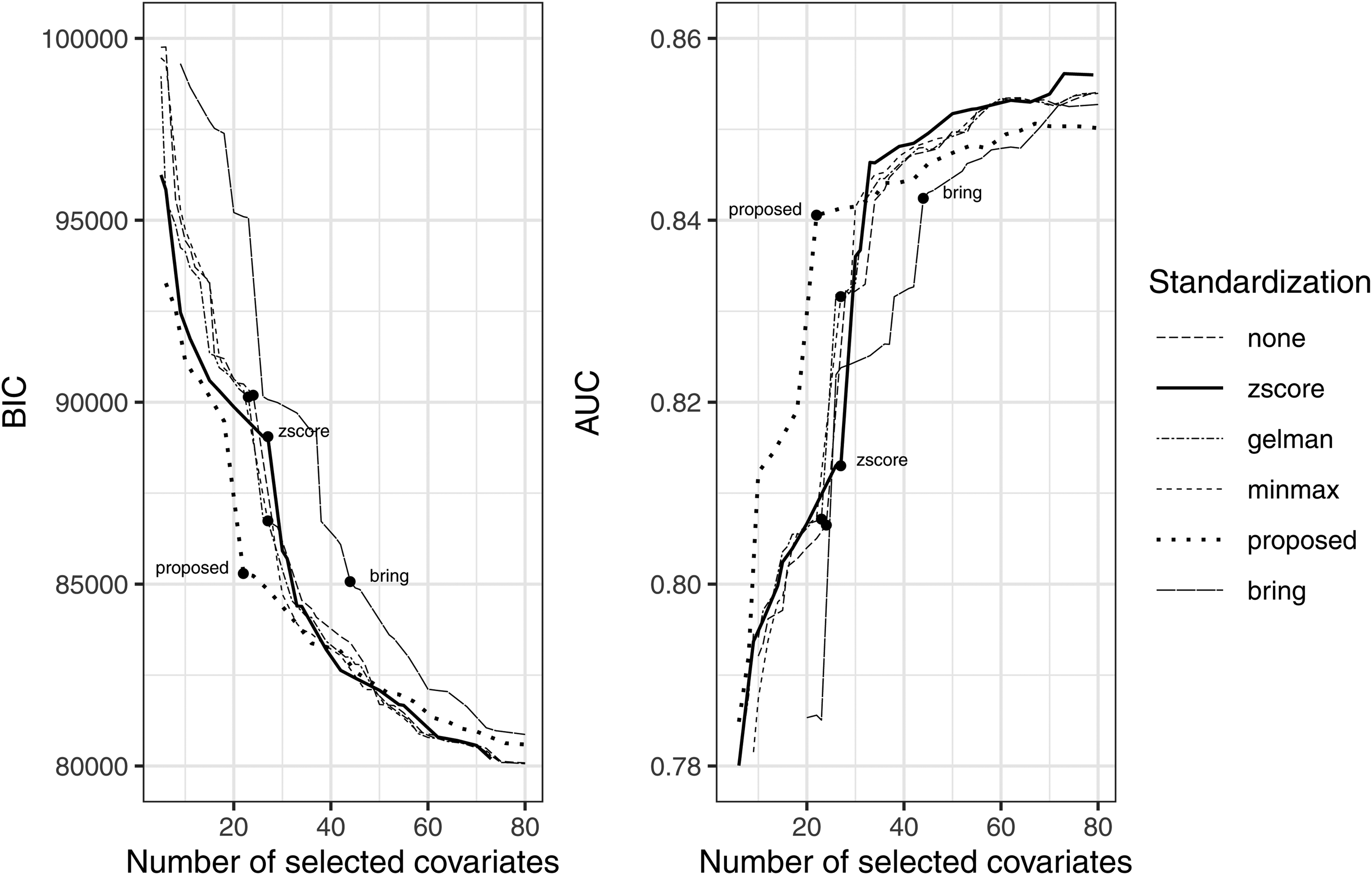
Plots of the BIC and AUC values versus the total number of selected covariates as penalty $λ$ decreases. Black points mark values corresponding to the $λ_{B I C_{1 s e}}$ .

Table 4.

NAMCS covariates selected by different standardization methods.

	None	Z-score	Gelman	Min–max	Bring	Proposed
Number of Selected Variables
Continuous	3	1	1	1	2	1
Binary	14	21	14	15	26	12
Multi-Category	7	5	8	11	16	9
Total	24	27	23	27	44	22
Model Performance with Selected Variables
$λ_{B I C_{1 s e}}$	383.50	1639.42	383.50	357.87	2482.86	1160.03
BIC $^{a}$	90189.60	89049.93	90144.88	86735.93	85068.13	85290.75
AUC $^{a}$	0.81	0.81	0.81	0.83	0.84	0.84
Log-Likelihood $^{a}$	$-$ 44896.71	$-$ 44336.09	$-$ 44860.53	$-$ 43059.32	$-$ 42114.85	$-$ 42345.94

$^{a}$ BIC, AUC and Log-likelihood are values at the selected $λ_{B I C_{1 s e}}$ .

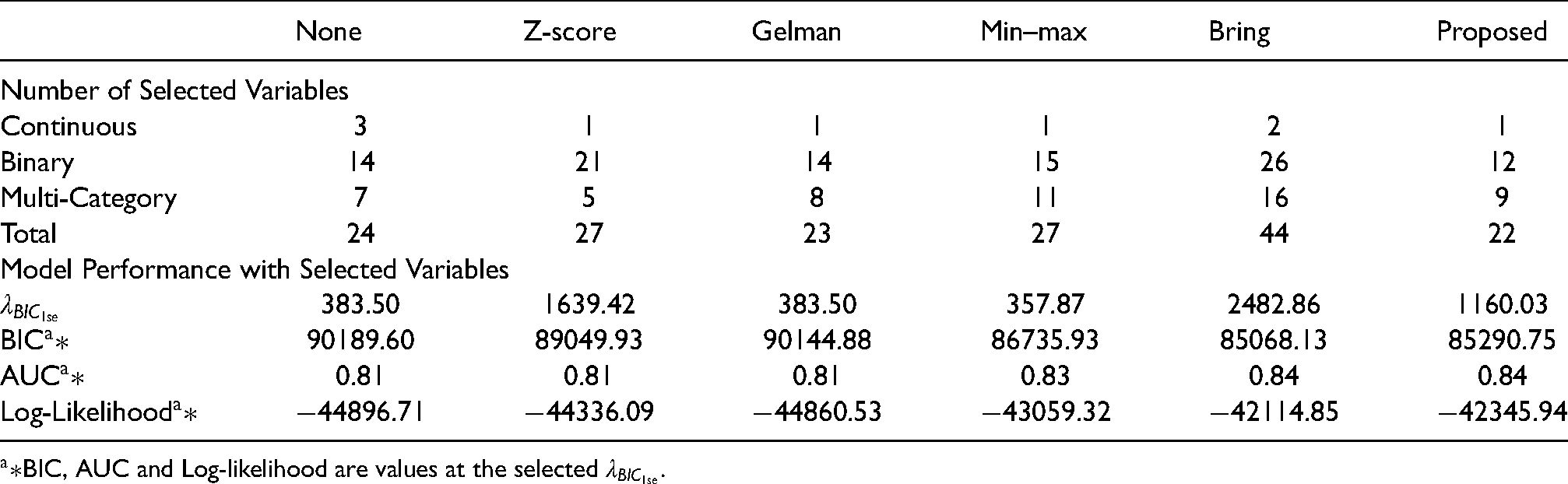
Figure 1 plots the BIC and AUC of the logistic model as more variables are selected by the penalized model using a sequence of decreasing $λ$ values. Different standardization methods are represented by different lines, and the black points indicate the BIC or AUC value at the selected $λ_{B I C_{1 s e}}$ . The plot shows that, at the selected $λ_{B I C_{1 s e}}$ values, Bring and the proposed method have better performance in terms of lower BIC values and higher AUC scores, compared to the other four standardization approaches. Furthermore, the proposed method has relatively better performance than all the other five standardization approaches, with lower BIC value and higher AUC score, and the least number of selected covariates. More interestingly, it also can be observed from the plots that in the left region where less variables are selected, the proposed method displays the consistent trend of lower BIC values and higher AUC scores.

In Table 4, we list the number of selected continuous, selected binary and selected multi-category variables, as well as the performance of logistic model using selected variables for each standardization method. There are some common patterns observed in both the simulation II and real data results: (1) With no standardization, continuous variables are more likely to be selected than with other standardization approaches. In real data, all three continuous variables are selected when no standardization is applied, while the other five standardization methods only have one or two continuous variable selected; (2) Z-score and Bring standardization approaches display similar behaviors. Binary variables with percentages of one close to 0.9 or 0.1 have higher chance of being selected in those two approaches compared with using the other methods. In real data, considering the fact that the majority binary variables have proportions of one greater than 0.9 or less than 0.1, 21, and 26 binary variables are selected in Z-score and Bring standardized data respectively, larger than the selection number of other methods; (3) Multi-category variables have the highest selection rates in Min–max and Bring methods. In real data, 11 and 16 multi-category variables are selected when Min–max and Bring standardization approaches are used, more than the numbers selected by other methods.

In addition, we have compared the covariates selected by different standardization methods with the 71 characteristics associated with opioid prescriptions proposed in St Clair et al.,²⁰ which identifies the characteristics based on the literature review, clinical relevance, and results from a random forest procedure on the 2015 NAMCS data (the present paper uses 2016 NAMCS data), and there are quite a few factors selected by both studies. Despite that the proposed method selects the least number of covariates, its selection set has more common covariates with St Clair et al.²⁰—16 common factors compared with 13 by None, Z-score, Gelman, Min–max methods and 19 by Bring method. It’s not surprising that Bring has more common factors with the reference study, but its selection performance is not necessarily better than the proposed methods, taking into account that Bring acutally selects twice as many factors as the proposed method. There are seven factors selected by all methods and the reference literature: number of medications other than the opioid prescribed to the patient, whether the patient’s injury occurs within 72 h prior to the visit, whether the patient has Arthritis, whether the doctor is the primary care provider to the patient, tobacco use of the patient, number of visits in the last 12 months of the patient, and depression of the patient.

5. Discussion

In the present study, we propose an alternative standardization method that aims to fairly select covariates of different types (i.e. continuous, binary, or categorical) in sparse penalized models. In the presence of covariates of different types in the same data set, we dichotomize continuous and multi-category variables to binary forms using a predefined percentile, then scale all binary covariates by their standard deviations. Our simulations show that the covariates with the same impact or association have comparable selection rates regardless of their data types by implementing the proposed standardization. In real data example, model using the proposed standardization has better BIC and AUC with the least number of predictors selected, compared to other standardization approaches.

Though dichotomization is common in clinical, epidemiology and social science research, the practice has always been controversial. Quite a few papers^8–10 criticized the practice of categorizing continuous covariates. However, most of the concerns focus on coefficient estimation and prediction accuracy. For instance, dichotomizing the continuous predictor when the underlying relationship with the outcome is continuous will lead to loss of power and loss of precision. And coefficient estimation can vary by the choice of cutoff points and sample data, sometimes the cutpoints are manipulated to generate over-optimistic P-values. We agree with those concerns, but would like to emphasize the important differences of the dichotomization implementation in the proposed method. First, the objectives are different. We focus on the variable selection instead of coefficient estimation. The cutoff point is not chosen to best discern outcome, alternatively, the choice is made to have the empirical probabilities consistent across the newly constructed (by dichotomization) binary variables and the observed binary variables. If coefficient estimation and prediction accuracy are of concern, one can always refit a model using the selected predictors in their original forms. Second, the assumptions are different. We assume that every observed covariate is generated from a latent continuous variable. That is, the observed continuous covariate is the same as the latent continuous variable, while the observed binary and multi-category covariates are categorized from latent continuous variables with unknown thresholds. Under such assumption, the standardization step of dichotomizing the observed continuous covariate aligns with the generation mechanism of the observed binary and multi-category covariates, which leads to the standardized coefficients reflective of the relationships between latent covariates and the outcome.

Various lasso extensions have been proposed to improve variable selection consistency. For example, the adaptive lasso²¹ and the lasso with nonconvex penalty,²² which maneuvers the penalties to achieve consistent variable selection. The block randomized adaptive iterative lasso (B-RAIL)⁷ reduces the influence of variation across mixed data types on the variable selection by alternating the algorithm. Compared with them, the present study tackles the variable selection from the perspective of data standardization, instead of model modification. Meanwhile, we admit that there are some limitations of the proposed standardization. For example, when regrouping the multi-category variable to binary form, we cannot guarantee the newly generated binary variable has percentage of one exactly equal to the specified value $p$ . Secondly, more theoretical works are needed to support Lemmas 1 and 2 with less idealized assumptions, which is a future research topic. Furthermore, the proposed standardization is only necessary when variable selection is dependent on the sizes of coefficients, for example, sparse penalized regressions. When variables are selected by P-value, coefficient of determination ( $R^{2}$ ) or likelihood, such as step-wise variable selection, the proposed standardization would not make any difference and the standardization is not necessary at all. The proposed standardization would not apply to non-sparse penalized models like the ridge regression, as the benefits of the proposed method all fall in the variable selection aspect, not coefficient estimates or outcome predictions. Ridge regression targets data with multi-collinearity and coefficient estimates with large variances, and leverages the trade-off between bias and variance to achieve smaller minimum squared error, so variable selection is not needed and dichotomization would hurt the model performance in prediction and accurate forms of the covariate effects. Nevertheless, in lasso penalized regression models, as demonstrated from the simulation results and real data analysis, the proposed standardization produces variable selection with a smaller number of covariates, lower BIC and higher AUC. The approach can be easily extended to other sparse penalized models, for instance, models with an elastic net penalty, or models with non-convex penalization functions.

Supplemental Material

sj-pdf-1-smm-10.1177_09622802221129042 - Supplemental material for Standardization of continuous and categorical covariates in sparse penalized regressions

Supplemental material, sj-pdf-1-smm-10.1177_09622802221129042 for Standardization of continuous and categorical covariates in sparse penalized regressions by Xiang Li, Yong Ma and Qing Pan in Statistical Methods in Medical Research

Footnotes

Acknowledgements

We gratefully acknowledge the computing resources provided on the High Performance Computing Cluster²³ operated by Research Technology Services at the George Washington University.

Declaration of conflicting interests

The authors declared no potential conflicts of interest with respect to the research, authorship, and/or publication of this article.

Funding

This work received funding support from the US Food and Drug Administration, Center for Drug Evaluation and Research, the Regulatory Science and Review Enhancement program. This manuscript reflects the views of the authors and should not be construed to represent the views or policies of the Food and Drug Administration.

ORCID iD

Xiang Li

Supplemental material

Supplemental material is available for this article online. A R package mixedStandardization has been developed for users to implement the five standardization methods (Z-score, Gelman, Min–max, Bring, and Proposed) mentioned in the paper, and is available for download at Github page .

References

Friedman

Hastie

Tibshirani

. Regularization paths for generalized linear models via coordinate descent. J Stat Softw 2010; 33: 1–22.

Breheny

Huang

. Coordinate descent algorithms for nonconvex penalized regression, with applications to biological feature selection. Ann Appl Stat 2011; 5: 232–253.

Suarez-Alvarez

Pham

Prostov

et al. Statistical approach to normalization of feature vectors and clustering of mixed datasets. Proc R Soc A 2012; 468: 2630–2651.

Gelman

. Scaling regression inputs by dividing by two standard deviations. Stat Med 2008; 27: 2865–2873.

Bring

. How to standardize regression coefficients. Am Stat 1994; 3: 209–213.

Nair

Hinton

. Rectified linear units improve restricted boltzmann machines. In Proceedings of the 27th International Conference on International Conference on Machine Learning. ICML’10, Madison, WI, USA: Omnipress. ISBN 9781605589077, pp. 807–814.

Baker

Tang

Allen

. Feature selection for data integration with mixed multiview data. Ann Appl Stat 2020; 14: 1676–1698.

Royston

Altman

Sauerbrei

. Dichotomizing continuous predictors in multiple regression: a bad idea. Stat Med 2006; 25: 127–141.

MacCallum

Zhang

Preacher

et al. On the practice of dichotomization of quantitative variables. Psychol Methods 2002; 7: 19–40.

10.

Harrell

. Categorizing continuous variables. https://discourse.datamethods.org/t/categorizing-continuous-variables/3.

11.

Centers for disease control and prevention. National ambulatory medical care survey data. https://www.cdc.gov/nchs/ahcd/index.htm (2016, accessed 01 September 2020).

12.

Tibshirani

. Regression shrinkage and selection via the lasso. J R Stat Soc Series B Stat Methodol 1996; 58: 267–288.

13.

Hastie

Tibshirani

Friedman

. The elements of statistical learning. 2nd ed. New York: Springer New York Inc., 2009. pp. 61–73.

14.

Yuan

Lin

. Model selection and estimation in regression with grouped variables. J R Stat Soc Series B Stat Methodol 2006; 68: 49–67.

15.

Meier

Van De Geer

Bühlmann

. The group lasso for logistic regression. J R Stat Soc Series B Stat Methodol 2008; 70: 53–71.

16.

Yang

Zou

. A fast unified algorithm for solving group-lasso penalized learning problems. Stat Comput 2015; 25: 1129–1141.

17.

Florentina

. Honest variable selection in linear and logistic regression models via

l 1

and

l 1 + l 2

penalization. Electron J Stat 2008; 2: 1153–1194.

18.

Centers for disease control and prevention. https://www.cdc.gov/drugoverdose/epidemic/index.html (2018, accessed 01 September 2020).

19.

National Center for Health Statistics. https://www.cdc.gov/nchs/nvss/vsrr/drug-overdose-data.htm (2021, accessed 01 November 2021).

20.

St Clair

Golub

et al. Characteristics associated with U.S. outpatient opioid analgesic prescribing and gabapentinoid co-prescribing. Am J Prev Med 2020; 58: e11–e19.

21.

Zou

. The adaptive lasso and its oracle properties. J Am Stat Assoc 2006; 101: 1418–1429.

22.

Fan

. Variable selection via nonconcave penalized likelihood and its oracle properties. J Am Stat Assoc 2001; 96: 1348–1360.

23.

Cluster TGWUHPC. Building a shared resource hpc center across university schools and institutes: a case study, 2020. https://arxiv.org/abs/2003.13629/. 2003.13629.

Supplementary Material

Please find the following supplemental material available below.

For Open Access articles published under a Creative Commons License, all supplemental material carries the same license as the article it is associated with.

For non-Open Access articles published, all supplemental material carries a non-exclusive license, and permission requests for re-use of supplemental material or any part of supplemental material shall be sent directly to the copyright owner as specified in the copyright notice associated with the article.

0.00 MB

0.18 MB

	$q = 0.5$		$q = 0.7$		$q = 0.9$
Standardization	Coefficient estimate	Ratio	Coefficient estimate	Ratio	Coefficient estimate	Ratio
None
$Z_{c o n t}$ $^{a}$	1.68 (0.43)		1.64 (0.43)		1.45 (0.36)
$Z_{b i}$ $^{a}$	2.65 (0.72)	0.66 (0.15)	2.72 (0.89)	0.63 (0.16)	6.02 (6.55)	0.48 (0.12)
Z-score
$Z_{c o n t}$	1.67 (0.44)		1.64 (0.44)		1.44 (0.38)
$Z_{b i}$	1.33 (0.36)	1.30 (0.31)	1.25 (0.41)	1.37 (0.35)	1.82 (1.98)	1.59 (0.40)
Gelman
$Z_{c o n t}$	3.35 (0.89)		3.27 (0.88)		2.89 (0.76)
$Z_{b i}$	2.65 (0.72)	1.31 (0.31)	2.72 (0.90)	1.26 (0.32)	6.03 (6.56)	0.96 (0.24)
Min–max
$Z_{c o n t}$	8.40 (2.36)		8.22 (2.35)		7.23 (2.02)
$Z_{b i}$	2.65 (0.72)	3.28 (0.81)	2.72 (0.90)	3.17 (0.85)	6.04 (6.57)	2.39 (0.62)
Bring
$Z_{c o n t}$	1.67 (0.44)		1.64 (0.44)		1.44 (0.38)
$Z_{b i}$	1.33 (0.36)	1.30 (0.31)	1.25 (0.41)	1.37 (0.35)	1.82 (1.98)	1.58 (0.40)
Proposed
$Z_{c o n t}$	2.15 (0.90)		1.95 (0.57)		2.94 (3.76)
$Z_{b i}$	2.17 (0.89)	1.03 (0.28) $^{b}$	1.93 (0.57)	1.05 (0.32)	3.11 (3.89)	1.07 (0.45)
$Z_{m u l t i}$	2.06 (0.85)	1.03 (0.31) $^{c}$	1.92 (0.66)	1.01 (0.30)	1.59 (0.67)	0.90 (0.38)