
Abstract
A range of chronic diseases have a significant influence on each other and share common risk factors. Comorbidity, which shows the existence of two or more diseases interacting or triggering each other, is an important measure for actuarial valuations. The main proposal of the study is to model parallel interacting processes describing two or more chronic diseases by a combination of hidden Markov theory and copula function. This study introduces a coupled hidden Markov model with the bivariate discrete copula function in the hidden process. To estimate the parameters of the model and deal with the numerical intractability of the log-likelihood, we use a variational expectation maximization algorithm. To perform the variational expectation maximization algorithm, a lower bound of the model’s log-likelihood is defined, and estimators of the parameters are computed in the M-part. A possible numerical underflow occurring in the computation of forward–backward probabilities is solved. The simulation study is conducted for two different levels of association to assess the performance of the proposed model, resulting in satisfactory findings. The proposed model was applied to hospital appointment data from a private hospital. The model defines the dependency structure of unobserved disease data and its dynamics. The application results demonstrate that the model is useful for investigating disease comorbidity when only population dynamics over time and no clinical data are available.
Keywords
Introduction
Comorbidity is a medical term that refers to when a patient has two or more diseases concurrently. A range of chronic diseases have a significant influence on each other and share common risk factors. Morbidity is more likely to result from complications caused by comorbid conditions than from the primary illness itself. 1 It can refer to a variety of chronic diseases that are highly interconnected and share risk factors.2,3
Statistical models have been used to identify patterns of co-occurrence of diseases.4–6 These studies, however, address the question of which comorbidities frequently co-occur but do not model their progression. Comorbidities are represented as networks using dynamic structural equation models.7,8 or deep diffusion processes. 9 The studies provide information on which diseases co-occur but not on the dynamics of diseases. Bayesian networks have been used to examine comorbidities and their temporal relationships.10–12 These works, which are based on a variety of different clinical and demographic data about patients, provide only a brief understanding of the underlying disease states representing the illness development. The interaction among diabetes and chronic liver disease under Metformin treatment is modeled by a coupled hidden Markov model (CHMM) with a personalized, non-homogeneous transition mechanism. 13 The model has a fixed number of hidden states but a greater number of states may be more informative about the progression of comorbidity. Also, the model is applied to clinical and demographic data, however, the application of the model to restricted administrative data may be limited.
Comorbidity is used in studies employing hidden Markov model (HMM) and its extensions.14–16 However, Markov models with memoryless properties imply that a patient’s current state is distinct from their future trajectory. As a result, HMM-based models are unable to adequately explain the variability in individuals’ progression trajectories, which are frequently caused by their varied clinical histories or chronologies (order and timing) of clinical events. This is a critical shortcoming in models of survival analysis for complex chronic diseases with numerous morbidities. 17
Our aim is to investigate these unknown shared factors that contribute to the development of these diseases. We are particularly interested in estimating the probability of chronic disease comorbidity, or how the presence of one disease may affect the likelihood of being exposed to another.
The theoretical set up in this study is mainly to combine hidden Markov and copula theories describing the probabilistic joint behavior of two or more chronic diseases. We use a CHMM as the fundamental model in this study to capture the comorbidity phenomenon by combining the hidden processes underlying chronic diseases. The causal nature of disease-disease interactions can be represented using dynamic networks, in which the strength of the edges connecting nodes varies over time in accordance to the joint copula distribution. The underlying network dynamics are frequently unknown, and what we perceive are sequences of observed events propagating across the network. To infer latent network dynamics from observed sequences, one must consider both when and what events occurred in the past, as both provide insight into the mechanisms behind disease generation and progression.
We propose a novel CHMM with copula accounting for interaction between diseases in the latent space. Since the hidden process of the CHMM is defined on a discrete state space, the probability of joint hidden states is modeled by bivariate discrete copula proposed by Geenens. 18 Sklar’s theorem states that the copula of a discrete random vector is not completely identifiable, resulting in serious inconsistencies. Therefore, Geenens 18 develops the rejuvenating approach of copula modeling for discrete data based on Yule’s, 19 Goodman and Kruskal’s, 20 and Mosteller’s 21 conceptions.
Several research have used copula theory to examine competing risks and comorbidity. While competing risks are investigated using a variety of copula-based approaches,22–26 there is only one study examining chronic disease comorbidity using a copula-based approach. 27 To our knowledge, no study has been conducted that uses a combination of any type of HMM and copula function to investigate comorbidity or competing risks.
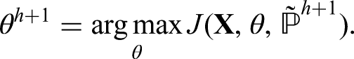
The proposed model is an incomplete data model for which the expectation maximization (EM) algorithm 28 is the most often used probability maximization technique. However, the model’s exact inference creates a number of computing problems. In this study, we define a probabilistic model in general form when the number of underlying hidden chains exceeds two, resulting in a large number of parameters. We employ variational approximation to make the expectation (E) step of the EM algorithm tractable in terms of computation. The resulting variational EM (VEM) seeks to maximize the lower bound on the log-likelihood. While VEM is initially formally described in machine learning applications such as Saul and Jordan, 29 it is now frequently deployed and generalized in a variety of ways. Comprehensive summary of studies can be found in the works of Jaakkola, 30 Blei et al., 31 Wainwright and Jordan. 32 Ormerod and Wand 33 gives also an explanation of VEM in statistical terms.
In this study, we present theoretical advances for defining a probabilistic model and developing the necessary inference to implement the model. In particular, we compute the complete data log-likelihood (CDLL) and its lower bound, derive forward–backward probabilities and conditional expectations required for the E-step, and derive estimators for the model parameters required for the maximization (M) step. We propose an approximate inference algorithm based on a variational approach. A simulation study is performed to assess the performance of the proposed method, and an application to the detection of comorbidity levels in heart diseases and hypertension is presented. In the study by Oflaz et al., 34 a latent Markov model with covariates influencing hidden states is used to examine the progression of ischemic heart disease (IHD). Extracted information on background factors leading to or influencing disease onset or progression is helpful for identifying hidden comorbidity levels of IHD and hypertension.
The proposed model takes into account the time influence of the disease improvement on the patient in both univariate and bivariate forms; exposes the factors having an impact on the diseases both in univariate and bivariate forms; controls the dependence structure in bivariate dimensions.
Interaction among diseases is implemented on limited administrative time series data not clinical data. It is critical to note that the majority of studies on competing risks rely on data from detailed clinical observations. However, a lack of data, particularly clinical data on individuals, may make classical statistical models of competing risks difficult to use. This could be due to restricted access to hospital data or a dearth of information on a particular cause or geographic location. As a result, it is necessary to develop alternative statistical models for sparse data.
Comorbidity of diseases have various etiological models, where risk factors have an influential role. 35 For example, in the associated risk factors model, risk factors for one disease are correlated with risk factors for another, increasing the likelihood of the diseases occurring concurrently. On the other hand, in the heterogeneity model, disease risk factors are not correlated, but each is capable of causing diseases associated with the other risk factor among diseases. The proposed model can be applicable to study various pathways to comorbidity, assuming that these interactions happen in an unobserved process.
Extensions of HMM
A strength of the HMM is that it can be readily extended to accommodate a variety of applications. In the literature, a linear combination of the prior estimate of the transition matrix and the empirical transition matrix is established by Siu et al., 36 Monte Carlo Markov chain is used to perform Bayesian inference and evaluate the posterior distribution of transition matrix. 37 The bivariate HMM have been developed to study the dependency between discrete and continuous observations. 38
There are established approaches to model interaction of several processes by combination of two or more HMMs. Hierarchical HMM is a model where each hidden state is an HMM as well, where children states depend on parent states. 39 Factorial HMM splits the hidden state into multiple variables that are merged at output, and each state has its own transition matrix. 40 Event-specific HMMs developed by Kristjansson et al., 41 aims to model a class of weakly connected time series in which only the onset of events are coupled in time. The representation capacity of event-coupled HMMs is clearly constrained by the restrictive structure, which is designed for a relatively narrow class of applications. Coupled HMM factor HMM to many chains in which the present state of each chain is dependent on the prior state of all chains. 42 Kwon and Murphy 43 models traffic velocities by using CHMM. Clearly, the completely coupled architecture developed by Brand et al. 42 is the most powerful in terms of representing interactions between many sequences. This framework can be used to naturally model a wide variety of applications. 44
Our model is distinguished by the fact that we combine interacting processes via a copula function, implying that joint hidden states follow a predefined joint probability. Other coupled HMMs with a variety of architectures combine hidden chains through the use of conditional probabilities; that is, hidden states are connected to preceding states following Markov property, and their distribution is defined solely by transition state probabilities. Assuming that hidden states are dependent on one another and have a joint probability distribution, and as we cannot observe hidden states directly, using a copula to represent the dependence structure is the optimal choice. Copulas have evolved into one of the most widely used statistical tools for describing, analyzing, and modeling the dependence of random variables.
There are several studies on integrating copula with an HMM. To construct a dependency between the intensity levels of the various modalities, a Gaussian copula is utilized, that is, marginal distributions of those are linked by a copula. 45 Another way of merging two theories is importing hidden Markov chain in the copula parameter. 46 Instead of the assumption of conditional independence between observed variables and hidden states researches suggest studying the dependence of observed values on unknown states via copula. 47 Also, there is a copula-based HMM of cylindrical time series, where a mixture of copula-based cylindrical densities approximates the distribution of cylindrical data, the parameters of which rely on the development of a latent Markov chain. 48 A copula is used to construct the dependence structure of the Markov process by providing copula representation of the Markov property. 49 To our best knowledge, there is no study that combines hidden chains using the copula function in the context of a coupled HMM.
Copula modeling for discrete random variables
Copulas are utilized to extract the dependency structure of a multivariate distribution. We can construct any multivariate distribution by providing the marginal distributions,
Due to issues with the copula function’s unidentifiability for discrete random variables, Geenens 18 proposes the bivariate discrete copula for count data. The existence and uniqueness of the proposed copula probability mass function is established.
In this study, the probability of joint hidden states is modeled by bivariate discrete copula, in particular we use bivariate binomial copula. With the constant trial numbers
For example, if

To be able to explain the joint behavior of two discrete time series variables, we combine two hidden Markov chains by copula function. For three or more time series variables, we suppose that there are identical number of hidden chains and we combine each pair of hidden chains by copula function. The proposed CHMM with discrete bivariate copula function accounts for dependency between diseases, it is a system of multiple interacting processes. The interaction between variables is considered in the hidden space rather than the observation space.
A series of observations
Emission distribution or state-dependent conditional distribution


Hidden Markov chain
We assume that the joint hidden process
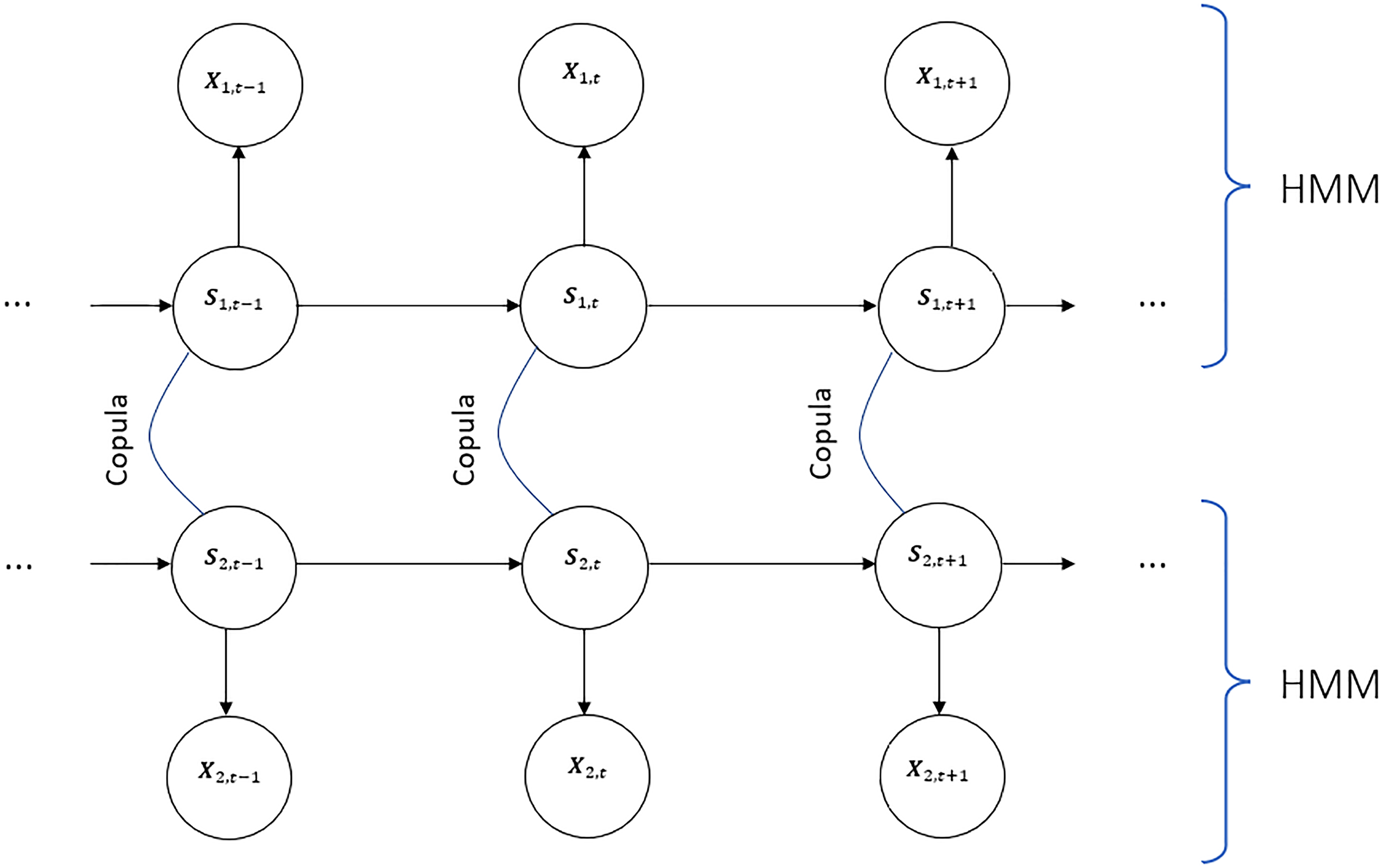
Directed graph of coupled hidden Markov model (CHMM) with copula function with two underlying Markov chains.
We assume that the transition probabilities of the joint hidden process the dependency relationship among the diseases is determined by the copula function, in particular,
In this model,

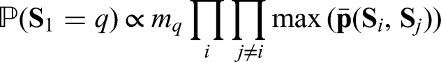
We further assume that the initial joint hidden process
The proposed method models the dependency of hidden chains by joint distribution of hidden states represented by discrete bivariate copula, whereas CHMM proposed by Brand et al. 42 couples chains by modeling the causal relationships between their hidden state variables with matrices of conditional probabilities.
The distribution of the hidden process
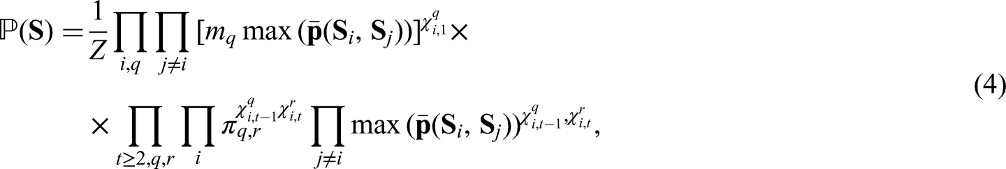
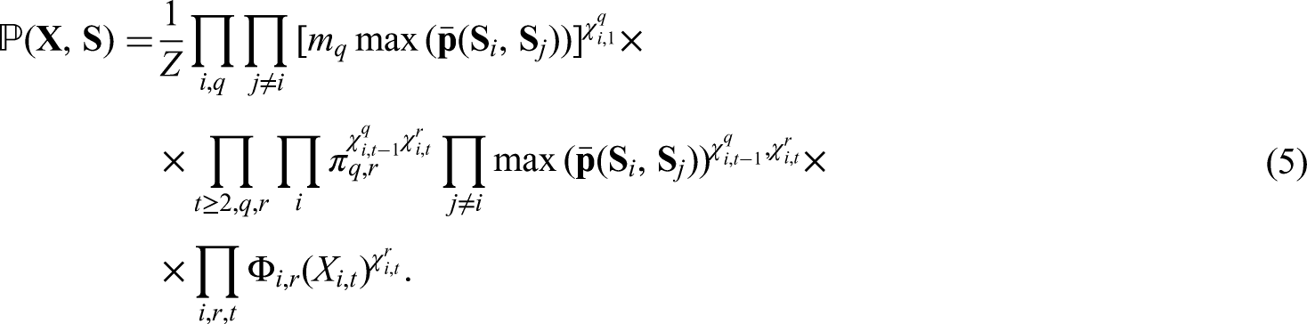
Therefore, the joint probability for the sequence of states and observations is defined as follows:
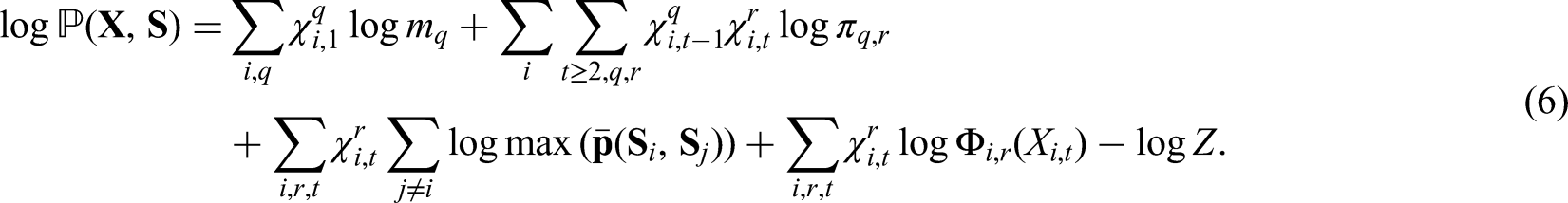
In the case of CHMM, where several hidden sequences are supposed to be dependent, the complexity of E-step becomes numerically inconvenient when number of parameters is too large. When both the number of chains and the number of states are small, that is, when
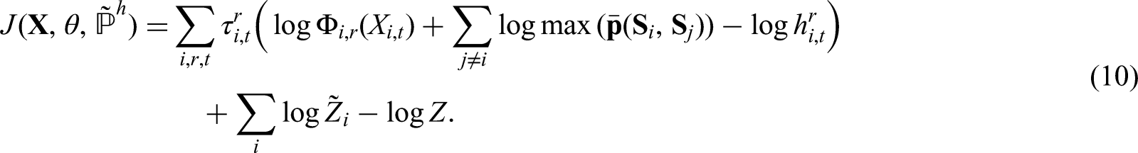
The VEM algorithm maximizes a lower bound of the log-likelihood. In the study, we mainly rely on the approach of Wang et al. 52 and follow the lines of Jaakkola, 30 Wainwright and Jordan 32 to derive the variational approximation of the log-likelihood.
For any distribution
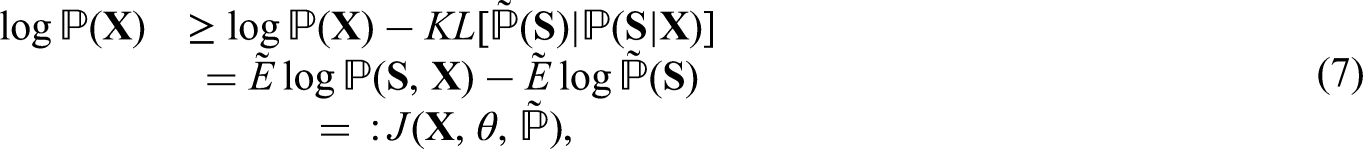


Let
Given observed random variable
Proof is provided in the Supplemental Material.
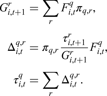
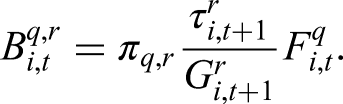
Based on these, we define analytically the optimal variation parameter in the E-part with the conditions for forward and backward algorithms.
Given observed random variable
Proof is provided in the Supplemental Material.
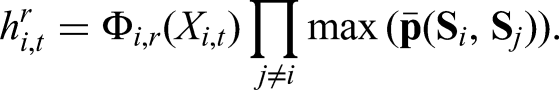
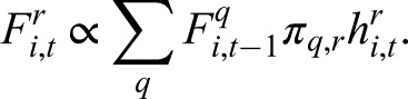
The conditional moment, which depend on the normalizing constant
Forward recursion: set
Given observed random variable


Proof is provided in the Supplemental Material.
Given observed random variable

Proof is provided in the Supplemental Material.
Given observed random variable
Proof is provided in the Supplemental Material.
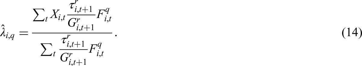
According to Wang et al.,
52
estimation of the dependency function within the M-step result in a poor estimation of the dependency function. The study suggests to use grid search of parameters and select the ones that minimize the weighted Residual Sum of Squares (RSS). Thus, we use the weighted RSS to select the optimal odds ratio,

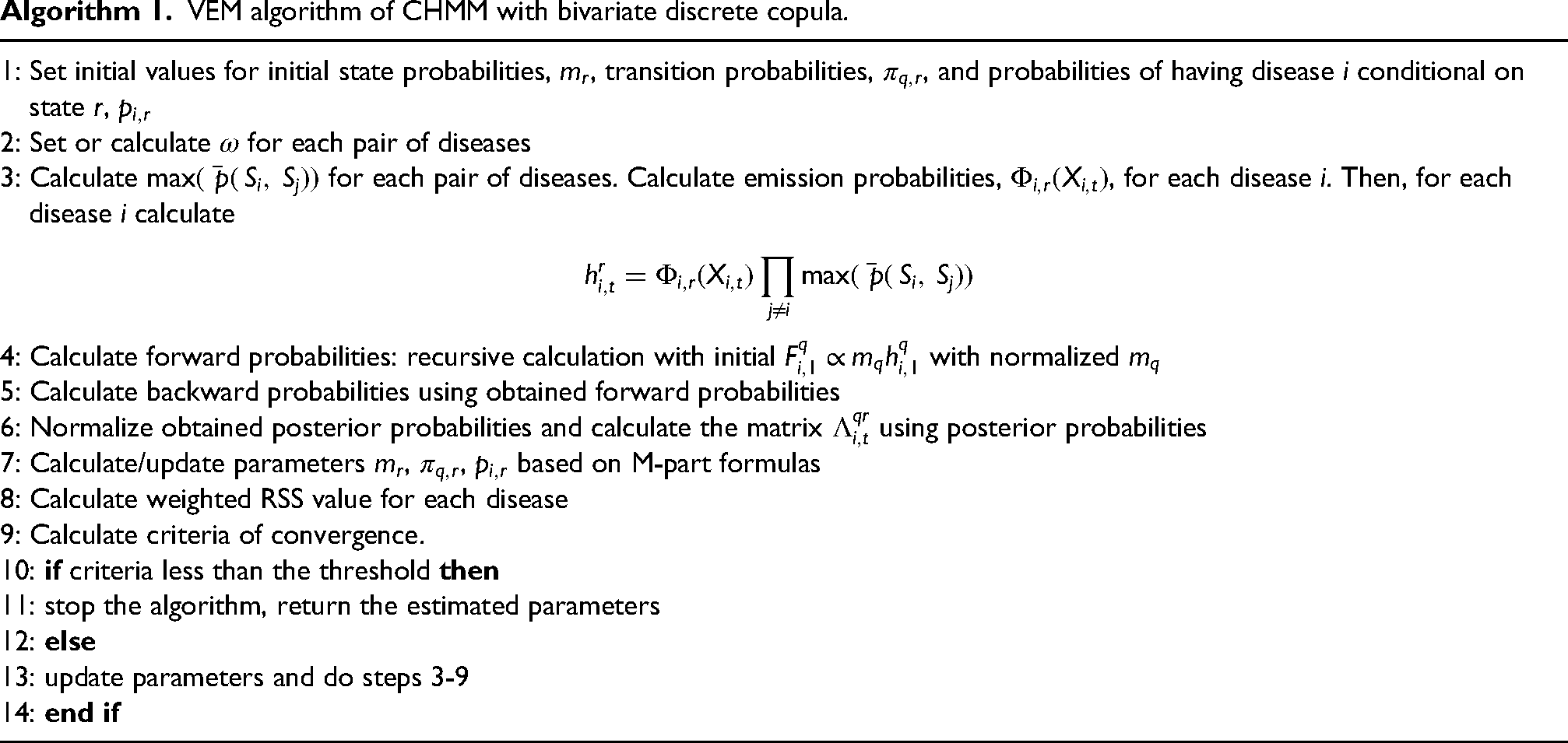
The proposed model is presented in algorithm to be more elaborated. The algorithm includes VE-part in steps 3 to 6, and the M-part in step 7.
VEM algorithm of CHMM with bivariate discrete copula.
VEM algorithm of CHMM with bivariate discrete copula.
The most frequently encountered problem in computing forward–backward probabilities, numerical underflow of the calculated probabilities, is resolved by transforming the functions used in the algorithm; additionally, scaling the observed values helps overcome numerical underflow. Precision is required when manipulating and executing arithmetic on small numbers. When possible, it is recommended to work with logarithms of probabilities. In particular, the “log-sum-exp” trick is useful when dealing with numerical underflow,55,31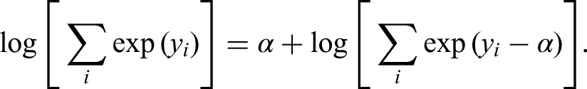
We conduct a simulation study that requires specific modeling to generate the comorbidity to capture the proposed model. Data sets with odds ratios of 0.85 and 8, which represent different correlation structures between the variables, are simulated.
For an odds ratio of 1, hidden states are independent. This scenario is inapplicable to the proposed model, as it is intended to model dependencies between hidden states. Additionally, when
When
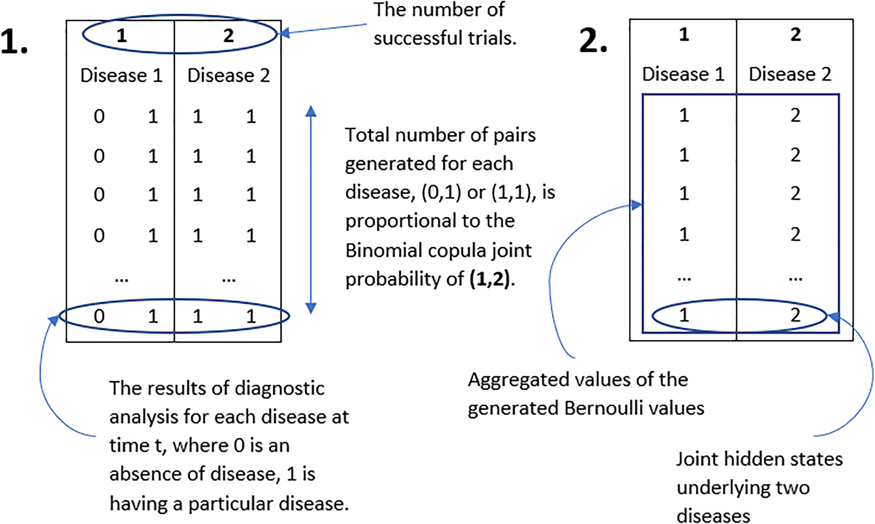
Simulation set up of hidden states for two diseases: generation and aggregation of Bernoulli values. For illustration purpose, only one out of eight possible pairs is displayed.
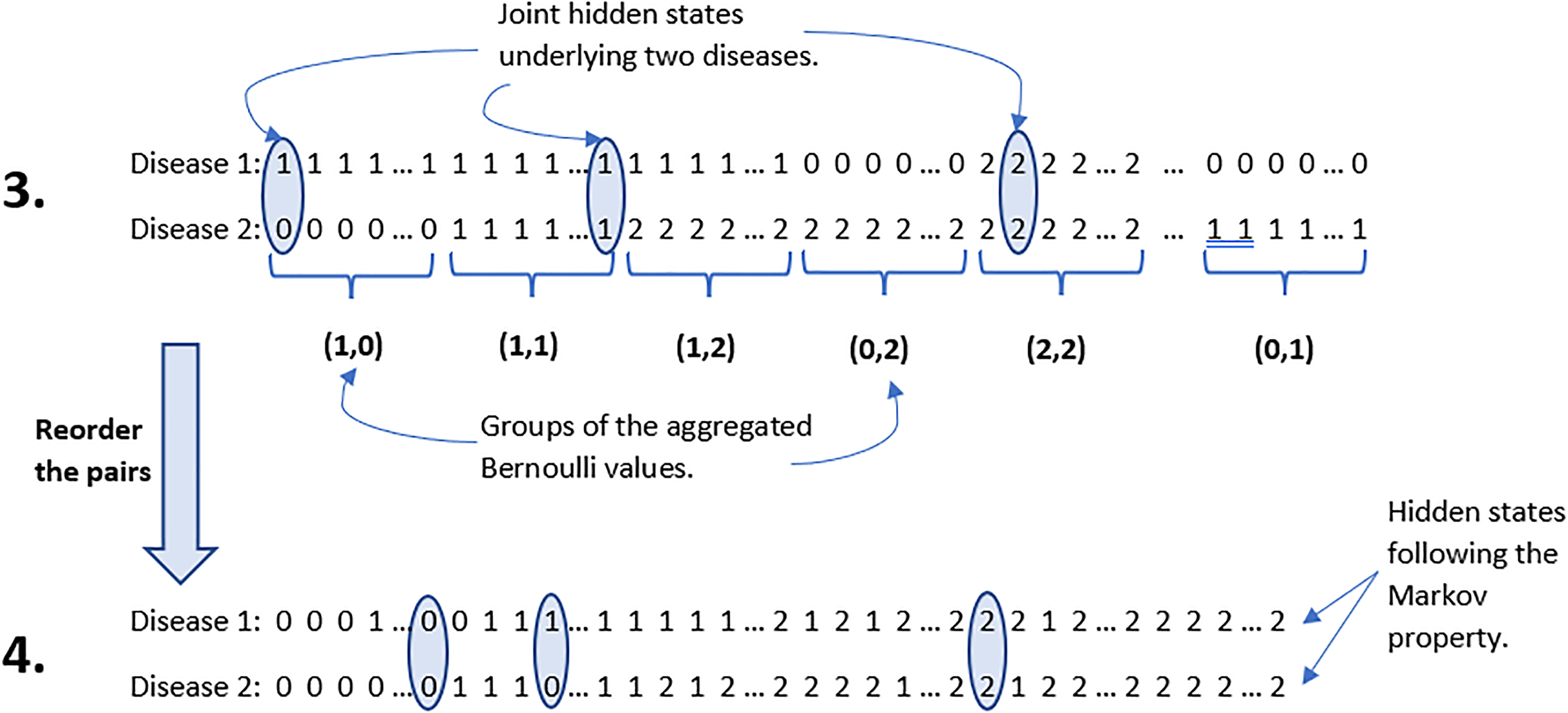
Simulation set up of hidden states for two diseases: reorder of the generated pairs.
We generate dependencies between the hidden chains using a bivariate Binomial copula, then observations dependent on hidden states are generated from a predefined distribution.
Calculate Binomial copula probabilities given a predefined odds ratio (equation (2)). For Generate joint states as explained in simulation set up for hidden states. The frequency of the generated joint states and Binomial copula probabilities given in equation (1) are compared based on bias and mean square error (MSE), Calculate transition probability matrices for each hidden chain. Aggregate probabilities of corresponding states and normalize by the total value in the corresponding row. Thus, the comorbidity transition matrix of the two diseases is obtained. Initial probability of the generated hidden states is defined as the frequency of the generated states at time Finally, generate observations from Poisson distribution given
To test whether the CHMM copula model optimally fits the simulated data, estimated transition, and initial probabilities, 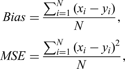
The three state hidden Markov chains representing two diseases are generated from Binomial copula distribution according to the simulation design. The order of the generated Bernoulli trials for each disease is such that the joint hidden states follow the Binomial copula and the sequence of hidden states for each disease follows the Markov property. For each disease, observed values were generated using a Poisson distribution with hidden state-dependent rate parameters. For odds ratios of
According to the chi-square-based Markovian test, 98.6% of the generated hidden states for disease
Proportion of stationary sequences among the 500 generated observations. Tests are conducted with significance level of 0.05. KPSS test for odds ratio of 8 also includes the results for significance level of 0.01.
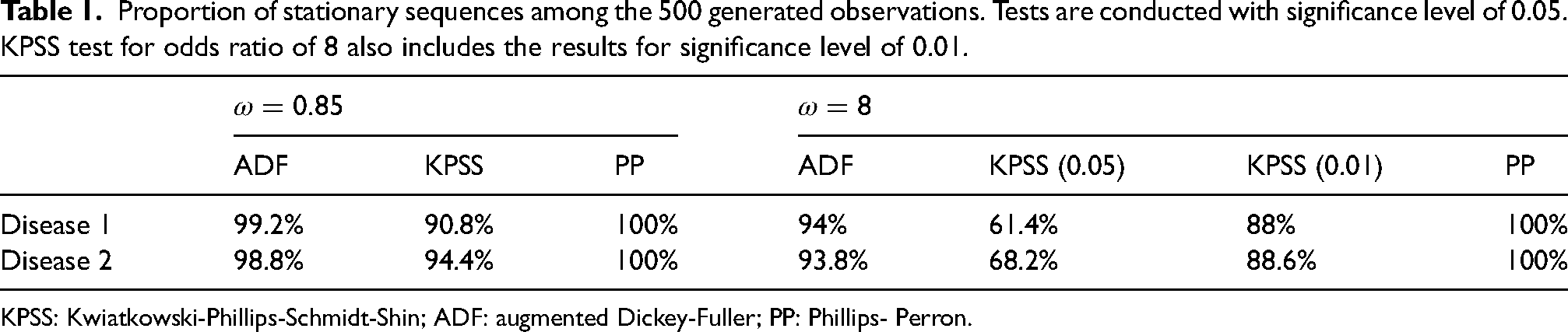
Proportion of stationary sequences among the 500 generated observations. Tests are conducted with significance level of 0.05. KPSS test for odds ratio of 8 also includes the results for significance level of 0.01.
KPSS: Kwiatkowski-Phillips-Schmidt-Shin; ADF: augmented Dickey-Fuller; PP: Phillips- Perron.
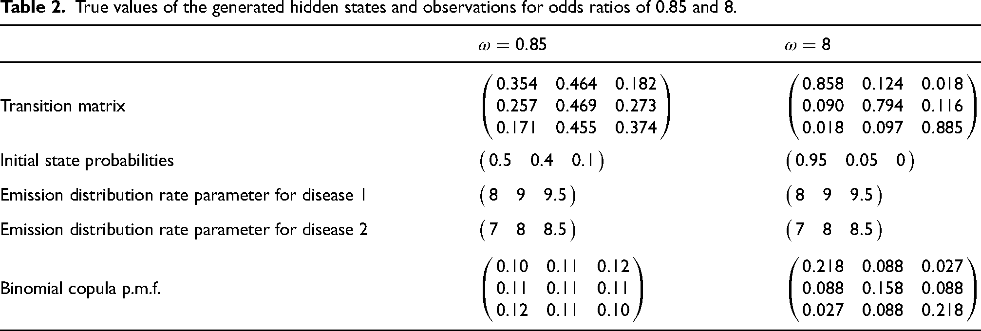
To distinguish estimated values of the generated data set from the estimated values by model, we call them true parameters of the generated data, see Table 2.
True values of the generated hidden states and observations for odds ratios of 0.85 and 8.
To assess the performance of the proposed model, 50 simulated data sets with the same parameters were used. Since the estimation of the parameters is an iterative process, we need to decide on the optimal iteration number to capture the best estimated results. Models with identical starting parameter settings but a varied number of inner iterations (70, 100, 150, 200, and 250) were applied to the simulated data sets.
The true values of the simulation design parameters are compared to the model’s estimated parameters using bias and MSE metrics. For clear demonstration of the model results on the simulated data, bias and MSE of the estimated parameters for each hidden state are calculated (see Tables 1 and 2 in the Supplemental Materials), and then mean of the values are displayed in Figure 4. Generally, for any number of iterations, the calculated bias and MSE between the estimated and true parameters of the simulation designs with an odds ratio of 0.85 and 8 are small, but for some cases we obtain moderately larger values. Having 16 parameters we aim to minimize the loss of the whole model while minimizing RSS, it is challenging to minimize the bias of all parameters. We assume that the general results of the simulation study are acceptable; however, it is difficult to find well-defined initial parameter settings that produce unbiased results due to a large number of parameters. The mean of MSE of the estimated and true rate parameters for both diseases of the simulated data with an odds ratio of 8 occasionally exceeds one. The values of error metrics vary depending on the initial and transition probabilities, as well as the emission distribution rate parameters.
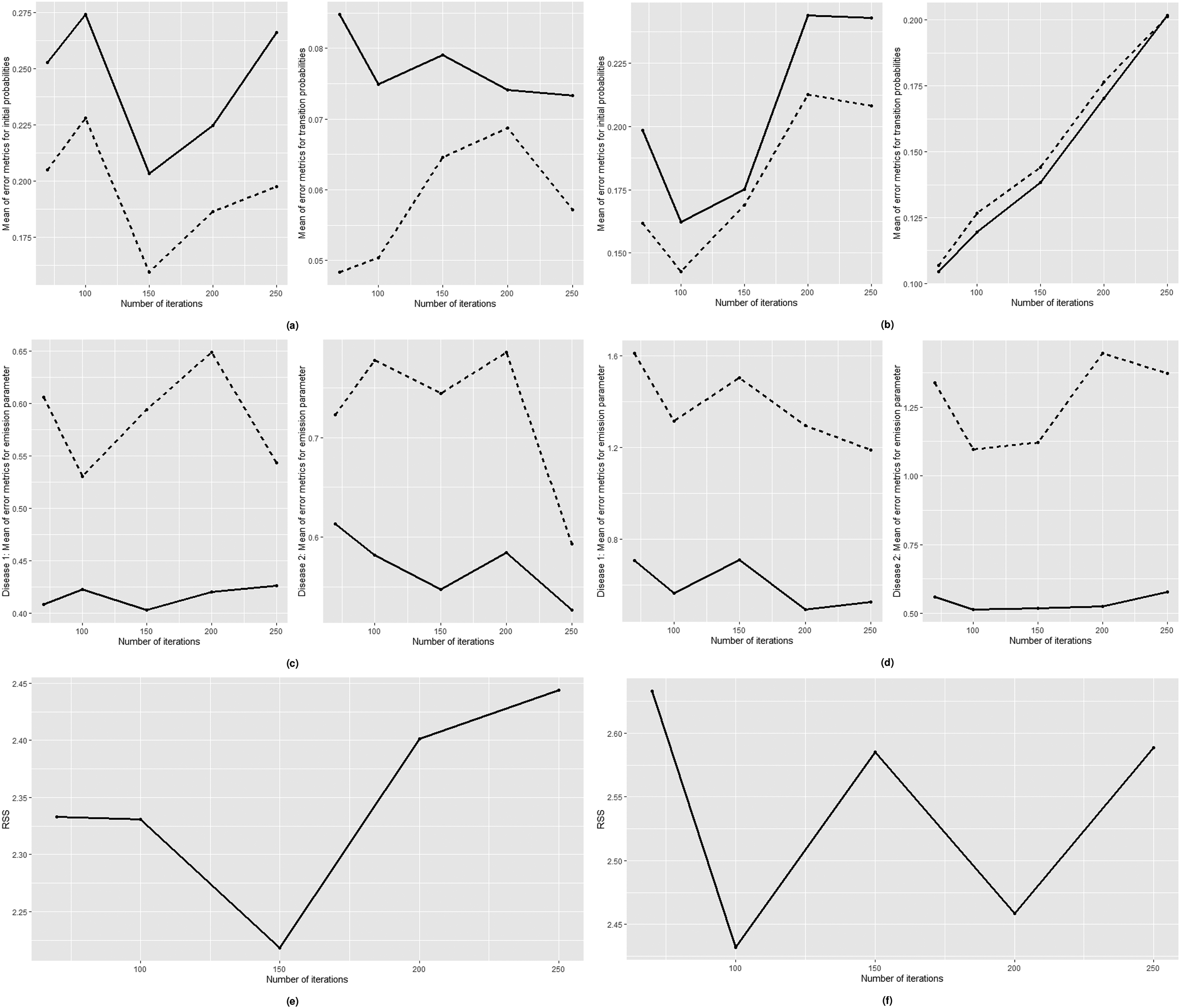
Mean of bias (dashed line) and MSE (solid line) of initial probabilities (left) and transition probabilities (right) for odds ratio of: a) 0.85 b) 8; mean of bias (dashed line) and MSE (solid line) of emission parameters for disease 1 (left) and disease 2 (right) for odds ratio of: c) 0.85 d) 8; weighted RSS values for odds ratio of: e) 0.85 f) 8. MSE: mean square error; RSS: Residual Sum of Squares.
The proposed model with 100 or 150 inner iterations number display the lowest bias and MSE values for parameters of the simulated data with an odds ratio of 0.85 (Figure 4(a) and (c)), the model with 100 iterations is the most optimal for data with an odds ratio of 8 (Figure 4(b) and (d)).
Additionally, the weighted RSS is used to evaluate the performance of models with varying iteration numbers. The weighted RSS exhibits the lowest value after 150 and 100 iterations for odds ratios of 0.85 and 8, respectively (Figure 4(e) and (f)). The weighted RSS values support the most optimal number of iterations for acquiring parameters close to their true values on average.
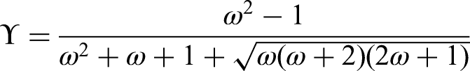
For simulated data with an odds ratio of 0.85 indicating a negative and close to zero Yule’s coefficient of association of
In this section of the study, we present the applicability of the proposed method onto the real data set. The data set includes daily information relating to the patients with heart disease and the hypertension collected from 49,713 patients from January 2015 to December 2020. Data set is authorized by a private hospital in Turkey, the observations are provided with confidentiality condition.
The illness codes of raw data set were classified into two categories: heart disease and hypertension. The repeated rows have been removed. The data contains information on integer age and gender, indicator variables for ever-diagnosed heart disease and hypertension since 2015, whether an individual was admitted to a hospital in a given month, and the frequency with which the patient presented to the hospital with heart disease or hypertension. Once a patient has been diagnosed with a disease, the value for that disease remains 1 for the remainder of the column. As the prehistory of individuals before 2015 is unknown, it is assumed that patients who do not appear in the system for the chosen period did not have a disease until their first hospital visit. After cleaning and transforming panel data, it was aggregated to create time series data by counting patients with heart disease or hypertension in each month from January 2015 to December 2020.
The total number of patients with heart disease or/and hypertension was analyzed using time series analysis and exploratory data analysis. Figure 5(a) and (b) depicts the time-series plots of the total number of patients with a specific disease divided by gender. Both diseases have an increasing trend due to assumptions that if a patient is reported to have a particular disease, he will be assumed to have that disease until the study is completed. For both diseases, male patients are increasing faster than female patients over time.
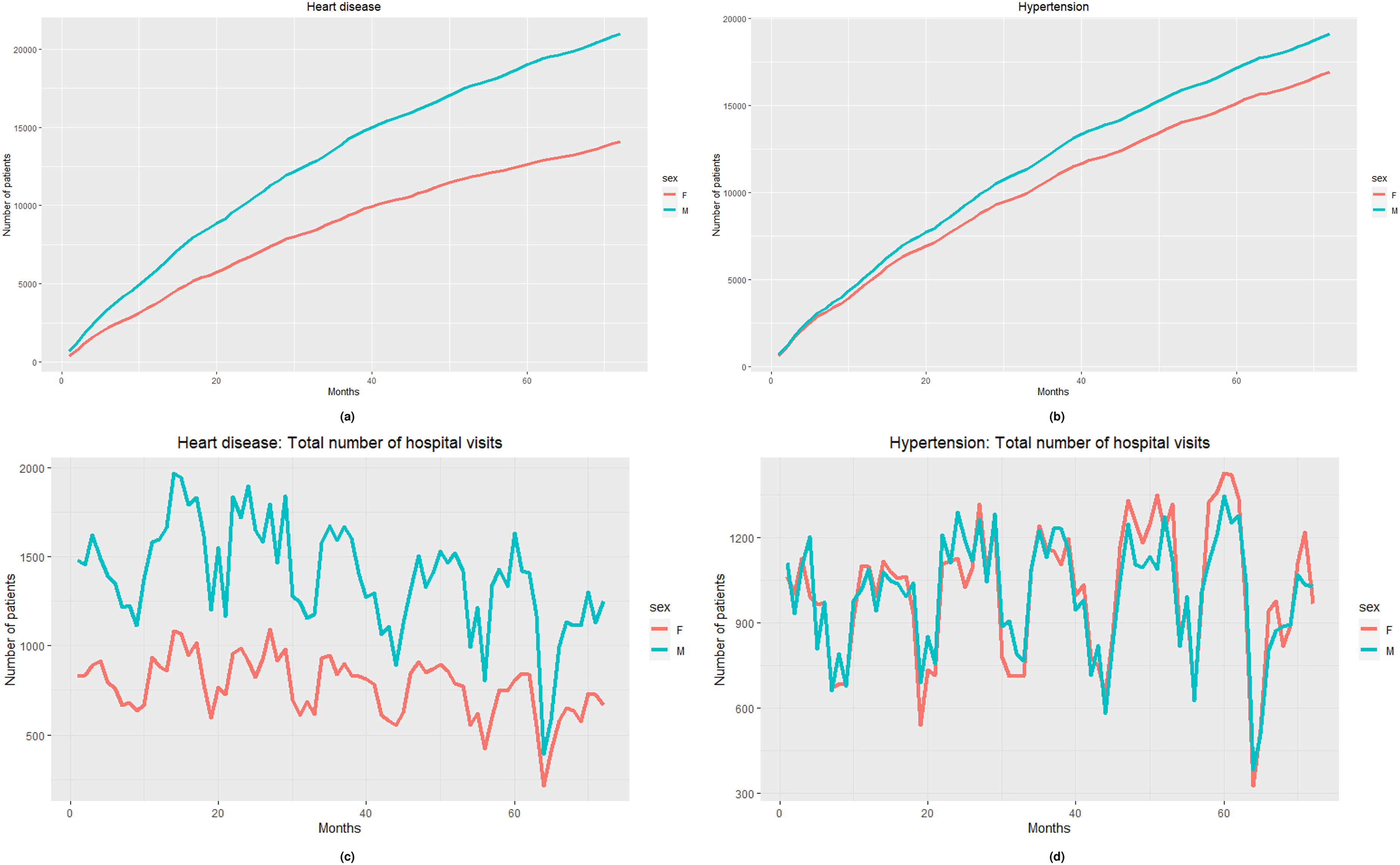
The number of patients by gender from January 2015 to December 2020 with: (a) heart disease, (b) hypertension. The number of hospital visits by gender from January 2015 to December 2020: (c) heart disease, and (d) hypertension.
Figure 5(c) and (d) shows the total number of hospital appointments for both diseases by gender. Hospital admissions for heart disease or/and hypertension follow a seasonal pattern. Females visit the hospital less frequently than males (check descriptive statistics), while hospital visits for patients with hypertension are comparable for both genders.
As illustrated in Figure 6(a) and (b), the number of patients with heart disease and hypertension, as well as patient hospital admissions, are highly linearly correlated. For both diseases, the total number of patients and their hospital visits follow a left-skewed distribution.
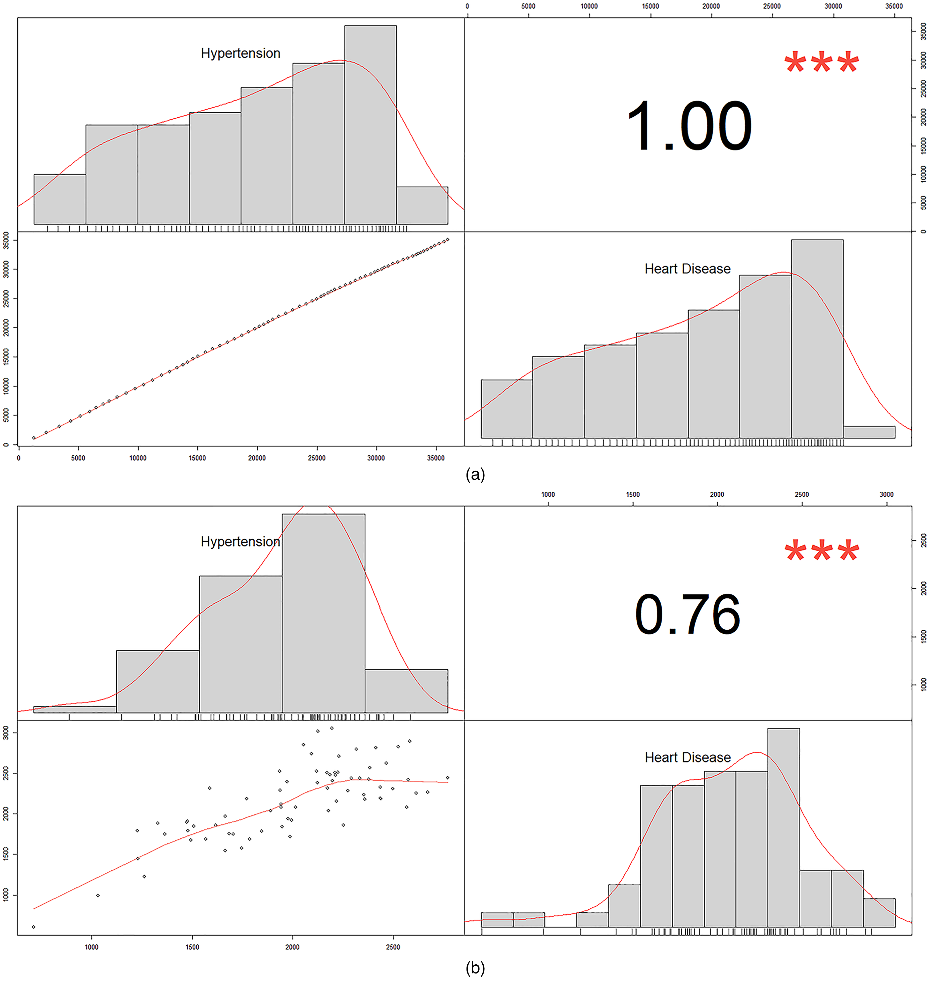
Heart disease and hypertension correlation plots and histograms: (a) patients number and (b) number of hospital visits.
We calculated the average time interval between disease occurrences. When hypertension occurs first, it takes an average of 12.96 months to be diagnosed with heart disease later; however, it takes an average of 18.88 months to be diagnosed with hypertension following heart disease. There are 4236 patients who develop heart disease after hypertension and 3108 patients who develop hypertension following heart disease.
Autocorrelation Function (ACF) and Partial Autocorrelation Function (PACF) plots of the total number of patients over 72 months and those with the second-order difference for both diseases are represented in Figure 7. The time series of patients number for both diseases are nonstationary, have an increasing trend.
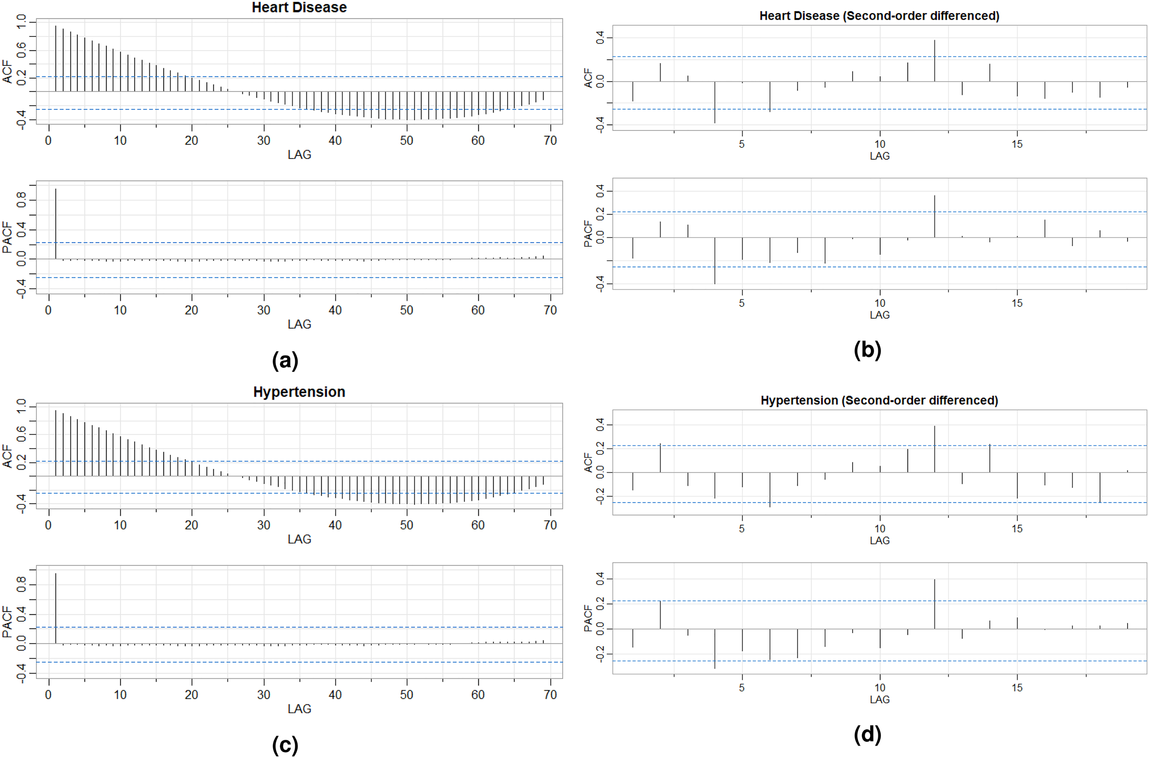
ACF and PACF plots of the number of patients over 72 months: (a) heart disease, (b) heart disease (second-order difference), (c) hypertension, and (d) hypertension (second-order difference). ACF: Autocorrelation Function; PACF: Partial Autocorrelation Function.
While HMMs are applicable to both stationary and nonstationary time series, 58 CHMMs, the proposed model’s underlying model, do not include any theoretical information indicating whether this type of model can be used for nonstationary time series. 42 Additionally, application studies used stationary series or transformed nonstationary ones to work with CHMM or models based on CHMM.59–62
A Kwiatkowski-Phillips-Schmidt-Shin (KPSS) test is used to determine the number of differences required to make time-series stationary at the significance level of 0.05. Second-order differencing is performed on the time series of both diseases based on the test results. According to Figure 7, heart disease and hypertension series with second-order lag are stationary. The augmented Dickey-Fuller (ADF) test with p-values less than 0.01 for both diseases, the KPSS test with p-values greater than 0.01 for both diseases, and the Phillips-Perron (PP) test with p-value of 0.01 for heart disease and hypertension indicate that the series are stationary.
The proposed model was applied to the number of patients with heart disease and hypertension resulting from the second-order differencing. Since the transformation produces negative values, the observations are increased by the minimum absolute value of the resulting observations, 270. Following that, the observed values are scaled by ten to obtain a stable VEM algorithm fit. These transformations does not affect the results because the aim is not to predict the number of patients but to predict the probability of co-occurrence. Initial setting for the model parameters are arranged as follows:
transition probability matrix with the initial state probability, rate parameters for emission distribution are arranged according to the mean and median values of the observations, the initial values set to
To obtain the model with the optimum fit, the odds ratios between two hidden states of the diseases, 
The estimated parameters of the model after 350 iterations for selected odds ratio of 70 are as follows:
transition probability matrix is initial state probabilities are emission distribution parameters of the state-dependent observations for heart disease and hypertension are
The weighted RSS value for the model is 10.38.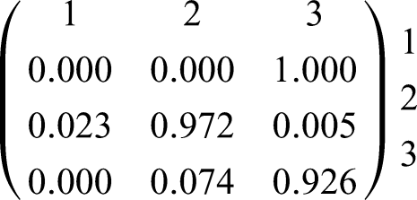
Interpretation of the findings
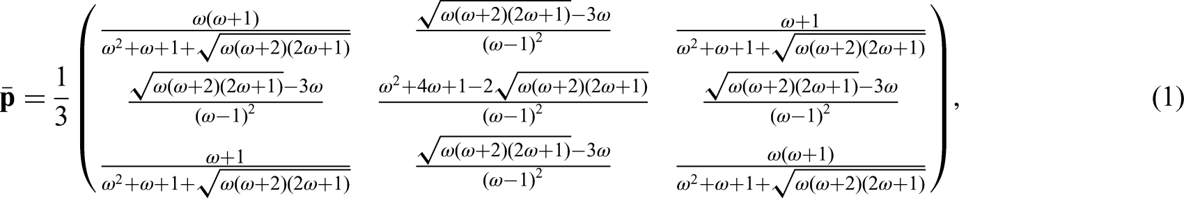
The Binomial copula distribution for estimated odds ratio of 70 is given as follows: State 2 represents no underlying risk factor; State 1 corresponds to the presence of one risk factor; State 3 corresponds to the presence of two risk factors.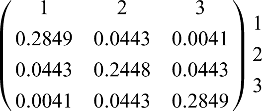
Relationships between comorbid diseases are described by various etiological associations.
35
We suppose that the occurrence of diseases at the same or different states may recognize the level of comorbidity between diseases. For example, if a single risk factor affects two diseases, that is, both diseases are on state 1, then we suppose that these diseases have a light comorbidity. If both risk factors affect both diseases, that is, hypertension and IHD are on state 3, then severe comorbidity exists. Figure 8 lists all possible interactions between diseases and risk factors.
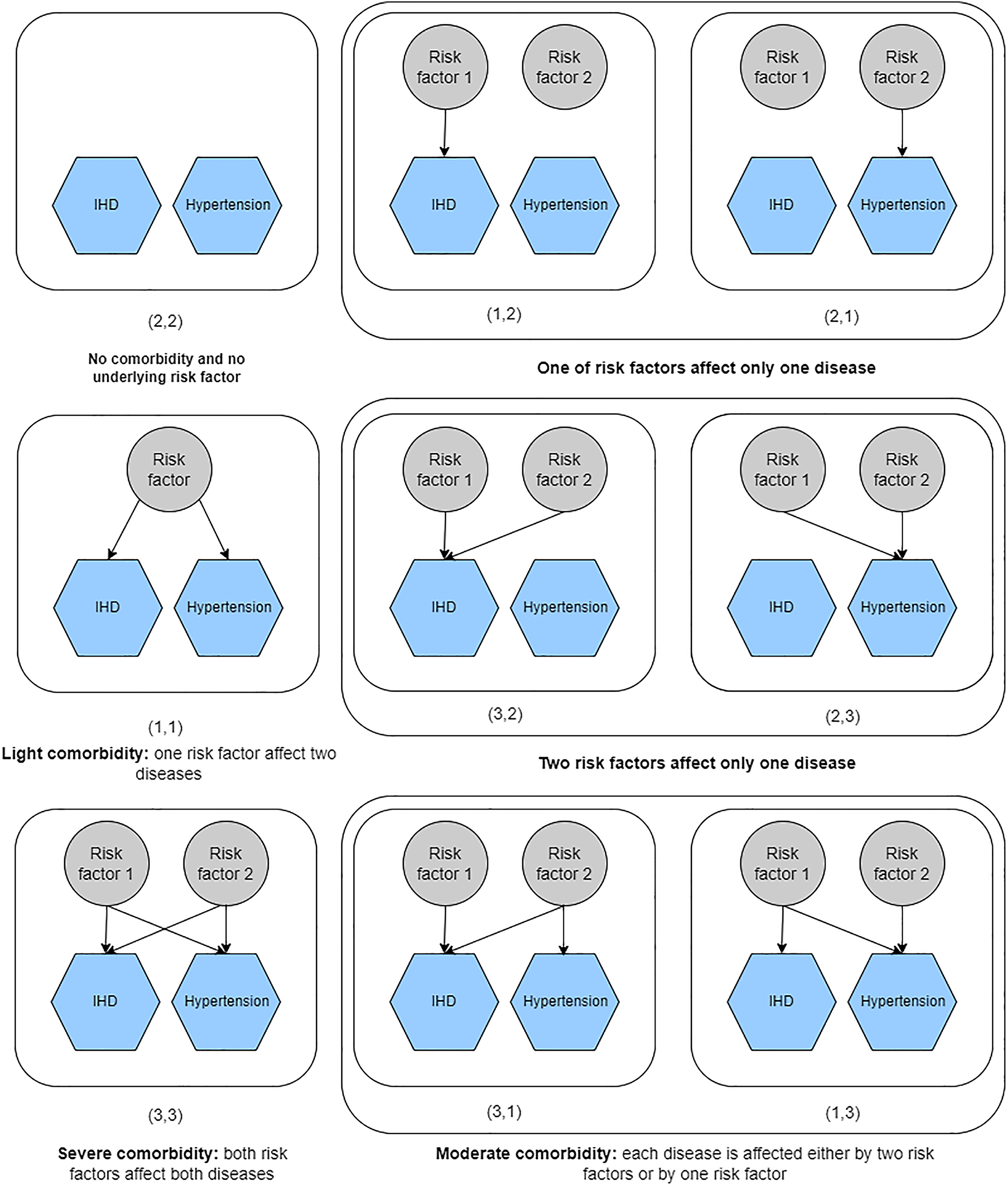
Interpretation of joint hidden states. Each structure relies on the interaction between diseases and risk factors.
According to the Binomial copula matrix, joint hidden states with different state numbers, such as
Figure 9 displays the example schemes for transitioning between joint hidden states. By multiplying the joint state and transition probabilities, we calculate the probability of moving from “no risk factor” to “one of risk factors affect one disease” level, that is, 

Example structure of joint hidden states with Binomial copula and transition probabilities.
The probability of both diseases remaining in “severe comorbidity,” that is, (3,3), is 0.2638. The probability of both diseases remaining in a “no risk factor,” that is, (2,2), is 0.2379. The probability of both diseases remaining in a “light comorbidity,” that is, (1,1), is 0.
The proposed model enables investigation of the joint behavior of hidden chains and hidden states, as well as their transition dynamics. Thus, we gain a better understanding of the dependency structure of unobserved knowledge regarding diseases with limited patient data based on hospital visits across time.
The main focus of the proposition in this study is to use a combination of hidden Markov theory and copula function to model parallel interacting processes describing two or more chronic diseases.
We develop a novel coupled HMM in this study that incorporates a bivariate discrete copula function into the hidden process. We employ a novel type of discrete copula, the Binomial copula. We compute a CDLL and develop the necessary inference to implement the model. Due to the large number of parameters required to estimate parameters using the EM algorithm, even for two hidden chains, estimation becomes computationally intractable. As a result, we estimate the model’s parameter using a VEM algorithm. Because the variational expectation part of the algorithm requires computing the lower bound approximation of CDLL, we use Kullback-Leibler divergence to derive the lower bound for the log-likelihood function based on the model. The VEM algorithm is carried out by computing conditional expectations based on forward-backward probabilities and estimators of parameters that maximize the CDLL.
Due to the unidentifiability of copula functions defined on discrete space, Geenens 18 developed a new bivariate discrete copula. Despite extensive theoretical development, statistical inference for parameter estimation of the joint copula function has not been developed yet. Thus, we designed a structure for joint states in such a way that they follow a predefined Binomial copula probability mass function with a given odds ratio while also satisfying the Markov property of hidden states in each chain. To verify and confirm the correctness of the designed structure, we calculated bias and MSE metrics and performed a Markovian test on 500 simulated data. The simulation study was conducted for two different odds ratio capturing weak and high association structure, and the developed model was applied. The findings of the simulation study are satisfactory.
The proposed model is applied to real data from a private hospital from January 2015 to December 2020, including information on hospital appointments. The observed variable is the total number of patients diagnosed with a particular disease in a given month. The purpose of this application is to define the dependency structure of unobserved clinical disease data. The application results demonstrate that the CHMM with discrete copula is useful for investigating disease comorbidity when only population dynamics over time are available and no clinical data are available.
During the application, one of the difficulties encountered is that the proposed model, like all HMM-based models, is sensitive to initial parameter settings. Because the developed model has a large number of parameters to estimate, the optimal fit is defined using combined information from weighted RSS. Additionally, the algorithm have been run multiple times with varying inner iteration counts in order to overcome a local optimum.
The model is applicable to the study of more than two diseases; more than two hidden chains can be included in the model. Additionally, the proposed model is general enough to account for any dependent events. The model can be extended to include covariates in both observed and hidden spaces. The proposed approach models interacting time-series observations; however, by combining CDLL and GLM functions, it is possible to extend this model to apply it to the longitudinal data.
Supplemental Material
sj-pdf-1-smm-10.1177_09622802231155100 - Supplemental material for Modeling comorbidity of chronic diseases using coupled hidden Markov model with bivariate discrete copula
Supplemental material, sj-pdf-1-smm-10.1177_09622802231155100 for Modeling comorbidity of chronic diseases using coupled hidden Markov model with bivariate discrete copula by Zarina Oflaz, Ceylan Yozgatligil and A Sevtap Selcuk-Kestel in Statistical Methods in Medical Research
Supplemental Material
sj-jpg-2-smm-10.1177_09622802231155100 - Supplemental material for Modeling comorbidity of chronic diseases using coupled hidden Markov model with bivariate discrete copula
Supplemental material, sj-jpg-2-smm-10.1177_09622802231155100 for Modeling comorbidity of chronic diseases using coupled hidden Markov model with bivariate discrete copula by Zarina Oflaz, Ceylan Yozgatligil and A Sevtap Selcuk-Kestel in Statistical Methods in Medical Research
Supplemental Material
sj-pdf-3-smm-10.1177_09622802231155100 - Supplemental material for Modeling comorbidity of chronic diseases using coupled hidden Markov model with bivariate discrete copula
Supplemental material, sj-pdf-3-smm-10.1177_09622802231155100 for Modeling comorbidity of chronic diseases using coupled hidden Markov model with bivariate discrete copula by Zarina Oflaz, Ceylan Yozgatligil and A Sevtap Selcuk-Kestel in Statistical Methods in Medical Research
Footnotes
Acknowledgements
This article is based on Ph.D. Thesis study by Oflaz Z. 68
Declaration of conflicting interests
The author(s) declared no potential conflicts of interest with respect to the research, authorship, and/or publication of this article.
Funding
The author(s) received no financial support for the research, authorship and/or publication of this article.
Supplemental material
Supplemental material for this article is available online.
References
Supplementary Material
Please find the following supplemental material available below.
For Open Access articles published under a Creative Commons License, all supplemental material carries the same license as the article it is associated with.
For non-Open Access articles published, all supplemental material carries a non-exclusive license, and permission requests for re-use of supplemental material or any part of supplemental material shall be sent directly to the copyright owner as specified in the copyright notice associated with the article.