Exact interval estimation for the linear combination of binomial proportions

Abstract

The weighted sum of binomial proportions and the interaction effect are two important cases of the linear combination of binomial proportions. Existing confidence intervals for these two parameters are approximate. We apply the $h$ -function method to a given approximate interval and obtain an exact interval. The process is repeated multiple times until the final-improved interval (exact) cannot be shortened. In particular, for the weighted sum of two proportions, we derive two final-improved intervals based on the (approximate) adjusted score and fiducial intervals. After comparing several currently used intervals, we recommend these two final-improved intervals for practice. For the weighted sum of three proportions and the interaction effect, the final-improved interval based on the adjusted score interval should be used. Three real datasets are used to detail how the approximate intervals are improved.

Keywords

Coverage probability interval length weighted sum of proportions interaction effect

1. Introduction

Consider $k$ independent binomials $X_{i} \sim B i n o (n_{i}, p_{i})$ for $i = 1, 2, \dots, k$ . The linear combination of binomial proportions,

λ = \sum_{i = 1}^{k} c_{i} p_{i}

(1)

for given constants

c_{i}

’s, is an important parameter of interest. For examples, the weighted sum of proportions and the interaction effect are often used in the field of biomedicine, and they are two special cases of

λ

The weighted sum of proportions requires $\sum_{i = 1}^{k} c_{i} = 1$ for positive $c_{i}$ ’s and is mainly applied to stratified data. For example, assume that the cure rate of a drug relates to the gender, and we know $c_{1}$ and $c_{2}$ , the male and female proportions in the population. Then the overall cure rate $λ$ is equal to the weighted sum of two cure rates of male and female $p_{1}$ and $p_{2}$ using the weights $c_{1}$ and $c_{2}$ . The interaction effect requires $\sum_{i = 1}^{k} c_{i} = 0$ for $c_{i} = 1$ or $- 1$ . It mainly studies the interaction effect between two factors. Here are two simple examples for the two cases.

Example 1

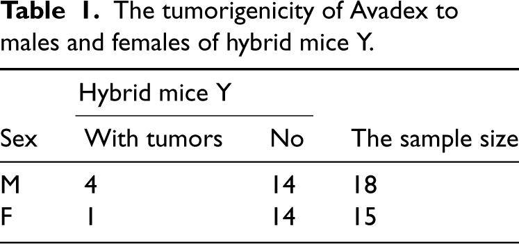
Innes et al.¹ tested the tumorigenicity of Avadex (a fungicide) by continuous oral administration to both males (M) and females (F) of hybrid mice Y. Table 1 contains the number of hybrid mice that develop the tumor in each sex group. The goal is to estimate the tumorigenicity of Avadex using the weighted sum of two proportions. The parameter of interest is the probability of the tumorigenicity of Avadex

λ = c_{1} p_{1} + c_{2} p_{2}

(2)

where

p_{1}

and

p_{2}

are the probabilities of the tumorigenicity of Avadex for males and females, respectively, and the weights of

c_{1}

and

c_{2}

are

3 / 8

and

5 / 8

, respectively.

Table 1.

The tumorigenicity of Avadex to males and females of hybrid mice Y.

	Hybrid mice Y
Sex	With tumors	No	The sample size
M	4	14	18
F	1	14	15

Example 2

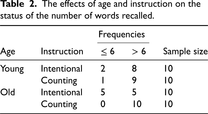
Bonett and Price² extracted a two-factor factorial design from Howell³ (1997, p. 404), where the factor A, age, is a two-level blocking factor (young and old) and the factor B, instruction, is also a two-level treatment factor (intentional and counting). The subjects in the study are classified into two categories by the number of words they recall: (i) less than or equal to six; and (ii) larger than six. The frequencies for four factor-level combinations are reported in Table 2. The parameter of interest is the interaction effect between age and instruction and is given in (17).

Table 2.

The effects of age and instruction on the status of the number of words recalled.

		Frequencies
Age	Instruction	$\leq 6$	$> 6$	Sample size
Young	Intentional	2	8	10
	Counting	1	9	10
Old	Intentional	5	5	10
	Counting	0	10	10

There have been efforts to derive confidence intervals for the linear combination of proportions $λ$ . Price and Bonett⁴ proposed the adjusted Wald interval that is simple to compute. Tebbs and Roths⁵ obtained a multivariate extension of the interval by Beal⁶ that focuses on $p_{1} - p_{2}$ . Zou et al.⁷ derived an interval based on the Wilson interval,⁸ and they claimed it is better than the adjusted Wald interval as the former has a coverage probability closer to the nominal level and a shorter interval length. Martín Andrés et al.⁹ proposed the score interval and several adjusted Wald-type approximate intervals. They recommended the score interval based on the numerical comparisons on coverage probability and interval length. Martín Andrés et al.¹⁰ further concluded that the score interval is the best in general, but the Wald3 interval (a variant of the Wald interval) is the best when the sample sizes are very small. Krishnamoorthy et al.¹¹ proposed the closed-form fiducial confidence interval, and they claimed that the interval is even better than the score interval.

There are also efforts on constructing confidence intervals for the weighted sum of proportions. A stratified Wilson interval was given by Yan and Su.¹² This interval is easy to compute and the confidence level of the interval is justified by extensive simulations. Decrouez and Robinson¹³ summarized seven confidence intervals for the weighted sum of two proportions that were originated from the intervals for the difference in two proportions. They recommended using the adjusted score interval for small samples, unless a simple calculation is important, in which case they advocated the Jeffreys–Perks interval.

The aforementioned intervals, however, are all approximate, and their confidence coefficients are less than the nominal level by significant amounts (see Tables 4, 5, and 8). To the best of our knowledge, the research on exact intervals for $λ$ , including the weighted sum and the interaction effect, is limited. Wang¹⁴ recently proposed the $h$ -function method, which can improve any given approximate interval to an exact one and uniformly shorten any given exact interval. Here, an interval is exact if it has an infimum coverage probability (ICP, also called the confidence coefficient) over the entire parameter space greater than or equal to the nominal level $1 - α$ , see Casella and Berger.¹⁵ Any confidence interval without this property is approximate. Lehmann and Romano¹⁶ (pp. 423–424) provided the definitions of the pointwise and uniformly asymptotically level $1 - α$ confidence intervals. The goal of this article is to derive exact intervals by applying the general $h$ -function method to two groups of intervals. The first group is for the weighted sum of two proportions and consists of six intervals described by Krishnamoorthy et al.¹¹ and Decrouez and Robinson;¹³ the second group is for the weighted sum of three proportions and the interaction effect and contains five intervals proposed by Price and Bonett,⁴ Zou et al.,⁷ Martín Andrés et al.,⁹ and Krishnamoorthy et al.¹¹ Then we choose the optimal exact interval from each group.

In Section 2, we describe five approximate intervals for $λ$ and the $h$ -function method for improving any given confidence interval. In Sections 3 and 4, the method is used to derive optimal exact intervals for the weighted sum of two and three binomial proportions, respectively. Section 5 focuses on the optimal exact interval for the interaction effect. Discussions are given in Section 6.

2. Preliminaries

Suppose we observe a random vector $\underline{X} = (X_{1}, \dots, X_{k})$ , where $X_{i}$ ’s are independent and each $X_{i}$ follows $B i n o (n_{i}, p_{i})$ for $i = 1, 2, \dots, k$ . Let ${\hat{p}}_{i} = X_{i} / n_{i}$ be the maximum likelihood estimator (MLE) of $p_{i}$ and let $p_{B} (x, n, p)$ be the probability mass function (PMF) of $B i n o (n, p)$ . The parameter and sample spaces are

H = {(p_{1}, p_{2}, \dots, p_{k}) : p_{i} \in [0, 1], i = 1, 2, \dots, k}

and

S = {(x_{1}, x_{2}, \dots, x_{k}) : x_{i} \in [0, n_{i}], i = 1, 2, \dots, k}

respectively. The linear function of binomial proportions, introduced in (1), is the parameter of interest. Let

C^{-} = \sum_{c_{i} < 0} c_{i}

and

C^{+} = \sum_{c_{i} > 0} c_{i}

. Then,

λ

belongs to a fixed interval

[C^{-}, C^{+}]

and has the MLE

\hat{λ} = \sum_{i = 1}^{k} c_{i} {\hat{p}}_{i} .

2.1. Five approximate intervals for $λ$

We describe five approximate intervals for $λ$ . These intervals are used to infer the weighted sum of proportions and interact effect in the next three sections, and they are to be improved by the $h$ -function method.

The first interval $C_{W a} (\underline{X})$ for $λ$ is the $1 - α$ adjusted Wald interval proposed by Price and Bonett⁴:

C_{W a} (\underline{X}) = \sum_{i = 1}^{k} c_{i} {\overset{˘}{p}}_{i} \mp z_{\frac{α}{2}} \sqrt{\sum_{i = 1}^{k} c_{i}^{2} \frac{{\overset{˘}{p}}_{i} (1 - {\overset{˘}{p}}_{i})}{(n_{i} + 4 / k)}}

(3)

where

{\overset{˘}{p}}_{i} = (X_{i} + 2 / k) / (n_{i} + 4 / k)

and

z_{\frac{α}{2}}

is the upper

\frac{α}{2}

-th percentile of the standard normal distribution.

The second interval $C_{W i} (\underline{X})$ is the modified Wilson interval proposed by Zou et al.⁷ Its lower and upper confidence limits are

\sum_{i = 1}^{k} c_{i} {\hat{p}}_{i} - \sqrt{\sum_{i = 1}^{k} [c_{i} {\hat{p}}_{i} - min (c_{i} L_{i}, c_{i} U_{i})]^{2}} and \sum_{i = 1}^{k} c_{i} {\hat{p}}_{i} + \sqrt{\sum_{i = 1}^{k} [c_{i} {\hat{p}}_{i} - max (c_{i} L_{i}, c_{i} U_{i})]^{2}}

(4)

respectively, where

L_{i} = \frac{{\hat{p}}_{i} + \frac{z_{\frac{α}{2}}^{2}}{2 n_{i}}}{1 + \frac{z_{\frac{α}{2}}^{2}}{n_{i}}} - \frac{z_{\frac{α}{2}}}{1 + \frac{z_{\frac{α}{2}}^{2}}{n_{i}}} \sqrt{\frac{{\hat{p}}_{i} (1 - {\hat{p}}_{i})}{n_{i}} + \frac{z_{\frac{α}{2}}^{2}}{4 n_{i}^{2}}} and U_{i} = \frac{{\hat{p}}_{i} + \frac{z_{\frac{α}{2}}^{2}}{2 n_{i}}}{1 + \frac{z_{\frac{α}{2}}^{2}}{n_{i}}} + \frac{z_{\frac{α}{2}}}{1 + \frac{z_{\frac{α}{2}}^{2}}{n_{i}}} \sqrt{\frac{{\hat{p}}_{i} (1 - {\hat{p}}_{i})}{n_{i}} + \frac{z_{\frac{α}{2}}^{2}}{4 n_{i}^{2}}}

The third interval

C_{S} (\underline{X})

, proposed by Martín Andrés et al.,⁹ is inverted from a family of the score tests, each test deals with the hypotheses:

H_{0} : λ = λ_{0} versus H_{A} : λ \neq λ_{0}

(5)

for a fixed value

λ_{0} \in [C^{-}, C^{+}]

. Let

l (λ, p_{1}, \dots, p_{k - 1}; \underline{x})

be the log-likelihood function in terms of

λ

p_{1}, \dots, p_{k - 1}

and let

{\tilde{p}}_{i} (λ_{0})

be the restricted MLE of

p_{i}

under

H_{0}

for

i = 1, \dots, k

. Introduce

v (λ_{0}, {\tilde{p}}_{1} (λ_{0}), \dots, {\tilde{p}}_{k - 1} (λ_{0})) = \sum_{i = 1}^{k} c_{i}^{2} \frac{{\tilde{p}}_{i} (λ_{0}) (1 - {\tilde{p}}_{i} (λ_{0}))}{n_{i}}

Then, the score test statistic is

T_{S} (\underline{x}, λ_{0}) = S^{2} (λ_{0}, {\tilde{p}}_{1} (λ_{0}), \dots, {\tilde{p}}_{k - 1} (λ_{0})) v (λ_{0}, {\tilde{p}}_{1} (λ_{0}), \dots, {\tilde{p}}_{k - 1} (λ_{0}))

where

S (λ_{0}, {\tilde{p}}_{1} (λ_{0}), \dots, {\tilde{p}}_{k - 1} (λ_{0})) = \frac{\partial}{\partial λ} l (λ_{0}, {\tilde{p}}_{1} (λ_{0}), \dots, {\tilde{p}}_{k - 1} (λ_{0}); \underline{x}) = \frac{x_{k} - n_{k} {\tilde{p}}_{k} (λ_{0})}{c_{k} {\tilde{p}}_{k} (λ_{0}) (1 - {\tilde{p}}_{k} (λ_{0}))}

The lower and upper confidence limits of the score interval

C_{S} (\underline{X})

are the solutions of

T_{S} (\underline{x}, λ_{0}) = z_{\frac{α}{2}}^{2}

as an equation in

λ_{0}

. Equivalently, the two confidence limits are solved by

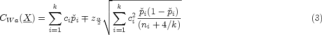
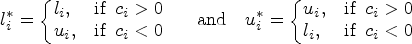
\frac{(\hat{λ} - λ_{0})^{2}}{v (λ_{0}, {\tilde{p}}_{1} (λ_{0}), \dots, {\tilde{p}}_{k - 1} (λ_{0}))} = z_{\frac{α}{2}}^{2}

(6)

The fourth interval

C_{A S} (\underline{X})

is the adjusted score interval, which is a variant of

C_{S} (\underline{X})

. A special case of this interval for

k = 2

was discussed by Decrouez and Robinson.¹³ Here, we extend the interval to any

k

. The confidence limits of the interval are obtained by solving the following equation in

λ_{0}

\frac{(\hat{λ} - λ_{0})^{2}}{v (λ_{0}, {\tilde{p}}_{1} (λ_{0}), \dots, {\tilde{p}}_{k - 1} (λ_{0}))} = z_{\frac{α}{2}}^{2} \frac{\sum_{i = 1}^{k} n_{i}}{\sum_{i = 1}^{k} n_{i} - 1}

(7)

Equations (6) and (7) are nearly identical except for an extra constant factor in the right-hand side of (7), which is due to Miettinen and Nurminen.¹⁷

The fifth interval $C_{F} (\underline{X})$ is the $1 - α$ fiducial interval proposed by Krishnamoorthy et al.¹¹:

C_{F} (\underline{x}) = [\hat{λ} - \sqrt{\sum_{i = 1}^{k} c_{i}^{2} ({\hat{p}}_{i} - l_{i}^{*})^{2}}, \hat{λ} + \sqrt{\sum_{i = 1}^{k} c_{i}^{2} ({\hat{p}}_{i} - u_{i}^{*})^{2}}]

(8)

with

\begin{aligned} l_{i}^{*} = {\begin{cases} l_{i}, & if c_{i} > 0 \\ u_{i}, & if c_{i} < 0 \end{cases} and u_{i}^{*} = {\begin{cases} u_{i}, & if c_{i} > 0 \\ l_{i}, & if c_{i} < 0 \end{cases} \end{aligned}

where

l_{i} = B_{x_{i} + 0.5, n_{i} - x_{i} + 0.5; 1 - \frac{α}{2}}

and

u_{i} = B_{x_{i} + 0.5, n_{i} - x_{i} + 0.5; \frac{α}{2}}

. Here,

B_{a, b; α}

denotes the upper

α

-th percentile of the Beta distribution with two positive shape parameters

a

and

b

2.2. The

h

-function method

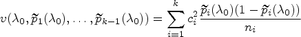
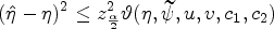
For a given initial interval for $λ$ , $C (\underline{X}) = [L (\underline{X}), U (\underline{X})]$ , Wang¹⁴ proposed the $h$ -function method which improves $C (\underline{X})$ of any level to an exact interval of level $1 - α$ , denoted by $C^{I} (\underline{X})$ ; if $C (\underline{X})$ itself is exact, then $C^{I} (\underline{X})$ is a subset of $C (\underline{X})$ . To derive $C^{I} (\underline{X})$ , introduce a test statistic $T_{C} (\underline{X}, λ_{0})$ for $H_{0}$ in (5) through $C (\underline{X})$

T_{C} (\underline{X}, λ_{0}) = min {λ_{0} - L (\underline{X}), U (\underline{X}) - λ_{0}}

(9)

where a small value of

T_{C} (\underline{x}, λ_{0})

supports

H_{A}

. The

h

-function based on

T_{C} (\underline{x}, λ_{0})

h_{C} (\underline{x}, λ_{0}) = sup_{H_{0}} P (T_{C} (\underline{X}, λ_{0}) \leq T_{C} (\underline{x}, λ_{0}))

(10)

Let

L^{I} (\underline{x}) = inf {λ_{0} : h_{C} (\underline{x}, λ_{0}) > α} and U^{I} (\underline{x}) = sup {λ_{0} : h_{C} (\underline{x}, λ_{0}) > α}

(11)

Then, the improved interval for

λ

at the sample point

\underline{x}

is given by

C^{I} (\underline{x}) = [L^{I} (\underline{x}), U^{I} (\underline{x})] .

The process of (9), (10), and (11) is the

h

-function method to improve

C (\underline{X})

in Wang.¹⁴ He proved two facts: (i)

C^{I} (\underline{X})

is exact for any interval

C (\underline{X})

, that is, the ICP of interval

C^{I}

satisfies

I C P (C^{I}) = inf_{H} P (λ \in C^{I} (\underline{X})) \geq 1 - α;

(ii)

C^{I} (\underline{X})

is contained in

C (\underline{X})

C (\underline{X})

is exact.

If we treat the one-time improved interval $C^{I} (\underline{x})$ as the initial interval and apply the $h$ -function method to it, then the two-time improved interval $C^{I 2} (\underline{x})$ is generated. Therefore, $C^{I 2} (\underline{x})$ is also exact and is a subset of $C^{I} (\underline{x})$ . We repeat this process for $m + 1$ times until $C^{I m} (\underline{x}) = C^{I (m + 1)} (\underline{x})$ . Then, $C^{I m} (\underline{x})$ is the final-improved interval by the $h$ -function method, denoted by $C^{I F} (\underline{x})$ . Wang¹⁴ proved that $C^{I F} (\underline{X})$ is a $1 - α$ exact interval and is a subset of $C^{I} (\underline{X})$ . Our numerical calculations show that a finite $m$ exists. In practice, if the lengths of $C^{I m} (\underline{x})$ and $C^{I (m + 1)} (\underline{x})$ are close enough for some $m$ , say their difference is <0.0001, then we stop the construction process and define $C^{I F} (\underline{x}) = C^{I m} (\underline{x})$ .

3. Exact intervals for the weighted sum of two proportions

In this section, we consider $k = 2$ in equation (1). Here, two independent $X_{1} \sim B i n o (n_{1}, p_{1})$ and $X_{2} \sim B i n o (n_{2}, p_{2})$ are observed. The parameter and sample spaces are

H_{1} = {(p_{1}, p_{2}) : 0 \leq p_{1}, p_{2} \leq 1} and S_{1} = {(x_{1}, x_{2}) : x_{1} \in [0, n_{1}], x_{2} \in [0, n_{2}]}

respectively. The parameter of interest is

η = c_{1} p_{1} + c_{2} p_{2}

, where

c_{1}

c_{2} > 0

and

c_{1} + c_{2} = 1

. Here, we use a new notation

η

to replace the general

λ

in (1), that is,

η

is the weighted sum of two proportions. Now,

η

has a range of

[0, 1]

. The MLE of

η

\hat{η} = c_{1} {\hat{p}}_{1} + c_{2} {\hat{p}}_{2}

Following the $h$ -function method, for any fixed $η_{0} \in [0, 1]$ , consider the hypotheses:

H_{0} : η = η_{0} vs. H_{A} : η \neq η_{0}

(12)

The null hypothesis

H_{0}

, in terms of

(p_{1}, p_{2})

, is equal to

{(p_{1} (p_{2}, η_{0}), p_{2}) : p_{2} \in D (η_{0})}

, where

p_{1} (p_{2}, η_{0}) = \frac{η_{0} - c_{2} p_{2}}{c_{1}} and D (η_{0}) = [max {\frac{η_{0} - c_{1}}{c_{2}}, 0}, min {\frac{η_{0}}{c_{2}}, 1}]

(13)

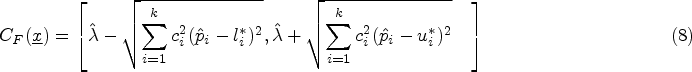
For a given interval

C_{η} (X_{1}, X_{2}) = [L_{η} (X_{1}, X_{2}), U_{η} (X_{1}, X_{2})]

for

η

, define a test statistic

T_{η} (X_{1}, X_{2}, η_{0}) = min {η_{0} - L_{η} (X_{1}, X_{2}), U_{η} (X_{1}, X_{2}) - η_{0}}

as in (9). Then, the

h

-function follows (10), i.e.

h_{η} (x_{1}, x_{2}, η_{0}) = sup_{p_{2} \in D (η_{0})} \sum_{{(u, v) \in S_{1} : T_{η} (u, v, η_{0}) \leq T_{η} (x_{1}, x_{2}, η_{0})}} p_{B} (u; n_{1}, p_{1}) p_{B} (v; n_{2}, p_{2})

This function looks complicated, but we give the details of calculation in Section 3.2. Find

L_{η}^{I} (x_{1}, x_{2}) = inf {η_{0} : h_{η} (x_{1}, x_{2}, η_{0}) > α}

and

U_{η}^{I} (x_{1}, x_{2}) = sup {η_{0} : h_{η} (x_{1}, x_{2}, η_{0}) > α}

. Then, the one-time improved interval (exact) is

C_{η}^{I} (x_{1}, x_{2}) = [L_{η}^{I} (x_{1}, x_{2}), U_{η}^{I} (x_{1}, x_{2})]

We repeat the improving process multiple times and obtain the final-improved interval

C_{η}^{I F} (X_{1}, X_{2})

, which is also exact and contained in

C_{η}^{I} (X_{1}, X_{2})

3.1. Improving six approximate intervals to exact intervals

We apply the above approach to improve the following five approximate intervals by Decrouez and Robinson¹³ and the fiducial interval by Krishnamoorthy et al.¹¹ to exact intervals, and further derive the corresponding final-improved intervals.

The first interval $C_{η 1}$ for $η$ is a special case of the adjusted Wald interval $C_{W a}$ in (3) when $k = 2$ . The second interval $C_{η 2}$ is the Jeffreys–Perks interval, which is obtained by solving the following inequality in $η$

(\hat{η} - η)^{2} \leq z_{\frac{α}{2}}^{2} ϑ (η, \tilde{ψ}, u, v, c_{1}, c_{2})

where

\tilde{ψ} = c_{1} \frac{n_{1} {\hat{p}}_{1} + 1 / 2}{n_{1} + 1} - c_{2} \frac{n_{2} {\hat{p}}_{2} + 1 / 2}{n_{2} + 1}, u = \frac{1}{4} (\frac{1}{n_{1}} + \frac{1}{n_{2}}), v = \frac{1}{4} (\frac{1}{n_{1}} - \frac{1}{n_{2}})

and

ϑ (η, \tilde{ψ}, u, v, c_{1}, c_{2}) = [(c_{1} + c_{2} - η) η + (c_{1} - c_{2} - \tilde{ψ}) \tilde{ψ}] u + [η (c_{1} - c_{2}) + \tilde{ψ} (c_{1} + c_{2}) - 2 η \tilde{ψ}] v

The third interval

C_{η 3}

needs the likelihood-ratio test statistic

Λ (x_{1}, x_{2}, η_{0}) = [{\frac{{\tilde{p}}_{1} (η_{0})}{{\hat{p}}_{1}}]}^{x_{1}} {[\frac{1 - {\tilde{p}}_{1} (η_{0})}{1 - {\hat{p}}_{1}}]}^{n_{1} - x_{1}} {[\frac{{\tilde{p}}_{2} (η_{0})}{{\hat{p}}_{2}}]}^{x_{2}} {[\frac{1 - {\tilde{p}}_{2} (η_{0})}{1 - {\hat{p}}_{2}}]}^{n_{2} - x_{2}}

where

{\tilde{p}}_{1} (η_{0})

is the restricted MLE of

p_{1}

under

H_{0}

and

{\tilde{p}}_{2} (η_{0}) = (η_{0} - c_{1} {\tilde{p}}_{1} (η_{0})) / c_{2}

. The interval is

C_{η 3} (x_{1}, x_{2}) = {η_{0} : - 2 \log (Λ (x_{1}, x_{2}, η_{0})) \leq z_{\frac{α}{2}}^{2}}

(14)

The intervals

C_{η 4}

C_{η 5}

, and

C_{η 6}

are the special cases of the score interval

C_{S}

in (6), the adjusted score interval

C_{A S}

in (7), and the fiducial interval

C_{F}

in (8), respectively, when

k = 2

. Decrouez and Robinson¹³ recommended

C_{η 5}

for small sample sizes. Krishnamoorthy et al.¹¹ claimed that

C_{η 6}

is better than

C_{η 4}

Table 3.

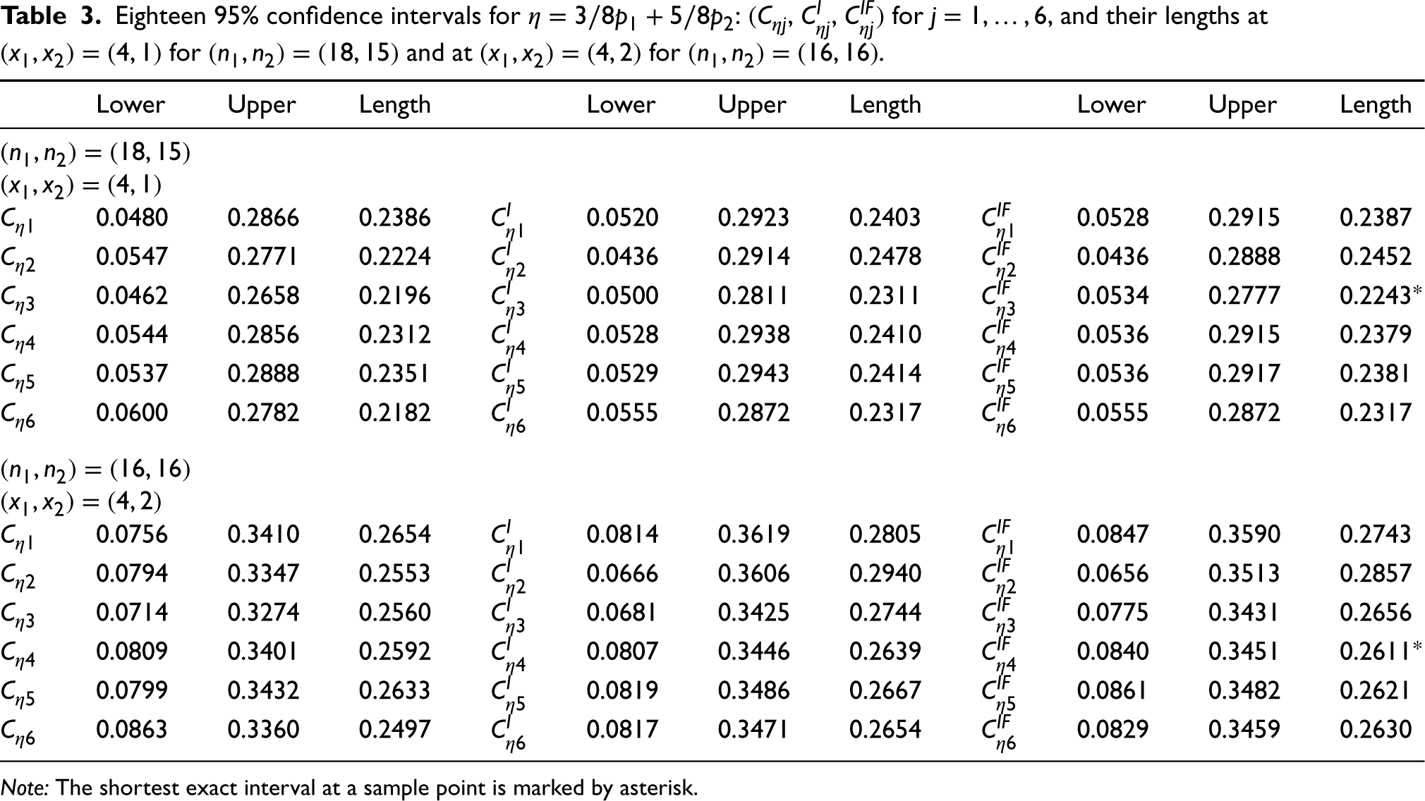
Eighteen 95% confidence intervals for $η = 3 / 8 p_{1} + 5 / 8 p_{2}$ : $(C_{η j}$ , $C_{η j}^{I}$ , $C_{η j}^{I F})$ for $j = 1, \dots, 6$ , and their lengths at $(x_{1}, x_{2}) = (4, 1)$ for $(n_{1}, n_{2}) = (18, 15)$ and at $(x_{1}, x_{2}) = (4, 2)$ for $(n_{1}, n_{2}) = (16, 16)$ .

	Lower	Upper	Length		Lower	Upper	Length		Lower	Upper	Length
$(n_{1}, n_{2}) = (18, 15)$
$(x_{1}, x_{2}) = (4, 1)$
$C_{η 1}$	0.0480	0.2866	0.2386	$C_{η 1}^{I}$	0.0520	0.2923	0.2403	$C_{η 1}^{I F}$	0.0528	0.2915	0.2387
$C_{η 2}$	0.0547	0.2771	0.2224	$C_{η 2}^{I}$	0.0436	0.2914	0.2478	$C_{η 2}^{I F}$	0.0436	0.2888	0.2452
$C_{η 3}$	0.0462	0.2658	0.2196	$C_{η 3}^{I}$	0.0500	0.2811	0.2311	$C_{η 3}^{I F}$	0.0534	0.2777	0.2243^*
$C_{η 4}$	0.0544	0.2856	0.2312	$C_{η 4}^{I}$	0.0528	0.2938	0.2410	$C_{η 4}^{I F}$	0.0536	0.2915	0.2379
$C_{η 5}$	0.0537	0.2888	0.2351	$C_{η 5}^{I}$	0.0529	0.2943	0.2414	$C_{η 5}^{I F}$	0.0536	0.2917	0.2381
$C_{η 6}$	0.0600	0.2782	0.2182	$C_{η 6}^{I}$	0.0555	0.2872	0.2317	$C_{η 6}^{I F}$	0.0555	0.2872	0.2317
$(n_{1}, n_{2}) = (16, 16)$
$(x_{1}, x_{2}) = (4, 2)$
$C_{η 1}$	0.0756	0.3410	0.2654	$C_{η 1}^{I}$	0.0814	0.3619	0.2805	$C_{η 1}^{I F}$	0.0847	0.3590	0.2743
$C_{η 2}$	0.0794	0.3347	0.2553	$C_{η 2}^{I}$	0.0666	0.3606	0.2940	$C_{η 2}^{I F}$	0.0656	0.3513	0.2857
$C_{η 3}$	0.0714	0.3274	0.2560	$C_{η 3}^{I}$	0.0681	0.3425	0.2744	$C_{η 3}^{I F}$	0.0775	0.3431	0.2656
$C_{η 4}$	0.0809	0.3401	0.2592	$C_{η 4}^{I}$	0.0807	0.3446	0.2639	$C_{η 4}^{I F}$	0.0840	0.3451	0.2611^*
$C_{η 5}$	0.0799	0.3432	0.2633	$C_{η 5}^{I}$	0.0819	0.3486	0.2667	$C_{η 5}^{I F}$	0.0861	0.3482	0.2621
$C_{η 6}$	0.0863	0.3360	0.2497	$C_{η 6}^{I}$	0.0817	0.3471	0.2654	$C_{η 6}^{I F}$	0.0829	0.3459	0.2630

Note: The shortest exact interval at a sample point is marked by asterisk.

3.2. A real-data analysis: Example 1 (continued)

The goal is to estimate the overall proportion of tumorigenicity of Avadex, $η = c_{1} p_{1} + c_{2} p_{2}$ , which is also given in (2). Assume the ratio of male to female is $3 : 5$ , then $c_{1} = 3 / 8$ and $c_{2} = 5 / 8$ .

For hybrid mice Y, as shown in Table 1, the dataset is $(x_{1}, n_{1}, x_{2}, n_{2}) = (4, 18, 1, 15)$ . Table 3 contains 18 intervals at the observed point $(x_{1}, x_{2}) = (4, 1)$ . Among the 12 exact intervals, the final-improved likelihood-ratio interval $C_{η 3}^{I F} (4, 1) = [0.0534, 0.2777]$ is the shortest among the exact intervals.

Innes et al.¹ were also interested in the tumorigenicity of Avadex of hybrid mice X. The observations are $(x_{1}, n_{1}, x_{2}, n_{2}) = (4, 16, 2, 16)$ and the associated intervals are given in Table 3 as well. In this case, the final-improved score interval $C_{η 4}^{I F} (4, 2) = [0.0840, 0.3451]$ is the shortest.

Next, we give the details of calculating the final-improved interval, for example, the above $C_{η 3}^{I F} (4, 1)$ .

Step 1: Following (14) compute the likelihood-ratio interval $C_{η 3} (x_{1}, x_{2}) = [L_{η 3} (x_{1}, x_{2}), U_{η 3} (x_{1}, x_{2})]$ for all sample points in $S_{1}$ . Here, there are 304 sample points. For example, $C_{η 3} (4, 1) = [0.0462, 0.2658]$ .

Step 2: We compute $C_{η 3}^{I} (4, 1)$ in this step. Let the test statistic $T_{η 3} (x_{1}, x_{2}, η_{0}) = min {η_{0} - L_{η 3} (x_{1}, x_{2}), U_{η 3} (x_{1}, x_{2}) - η_{0}}$ as in (9). Following (10), the $h$ -function at $(x_{1}, x_{2}) = (4, 1)$ is

h_{η 3} (4, 1, η_{0}) = sup_{p_{2} \in D (η_{0})} \sum_{{(u, v) \in S_{1} : T_{η 3} (u, v, η_{0}) \leq T_{η 3} (4, 1, η_{0})}} p_{B} (u; n_{1}, p_{1} (p_{2}, η_{0})) p_{B} (v; n_{2}, p_{2})

where

p_{1} (p_{2}, η_{0})

and

D (η_{0})

are given in (13). Then, we find the smallest and largest solutions of

h_{η 3} (4, 1, η_{0}) > 0.05

and obtain

C_{η 3}^{I} (4, 1) = [L_{η 3}^{I} (4, 1), U_{η 3}^{I} (4, 1)] = [0.0500, 0.2811]

. Two specific steps of computing

h_{η 3} (4, 1, η_{0})

for any

η_{0}

and finding the smallest and largest solutions of

h_{η 3} (4, 1, η_{0}) > 0.05

are as follows:

Step 2-1: Computing $h_{η 3} (4, 1, η_{0})$ at a fixed $η_{0}$ involves finding a global supremum of the summation in the right-hand side of the previous equation when $p_{2}$ runs over set $D (η_{0})$ . First, we use the grid search method to search for a maximum point, say $p_{20}$ , that maximizes the summation on an evenly distributed subset of $D (η_{0})$ . Then, we find the local maximum of the summation within a small neighborhood of $p_{20}$ by the function “optimize” in R. If the subset is dense enough in $D (η_{0})$ , then the local maximum is equal to the target value $h_{η 3} (4, 1, η_{0})$ . For example, when $η_{0} = 0.3$ , $D (0.3) = [0, 0.48]$ , $p_{2}$ runs over this range with a step of length 0.0005, and $h_{η 3} (4, 1, 0.3) = 0.0253 \leq 0.05$ .

Step 2-2: The range of $η_{0}$ is $[0, 1]$ . To find the smallest root, $L_{η 3}^{I} (4, 1)$ , of $h_{η 3} (4, 1, η_{0}) > 0.05$ , we start the search from 0 to 1 in a lattice manner and find the local root by the function “uniroot” in R. For example, if using the step length of 0.0005, we compute $h_{η 3} (4, 1, η)$ , where $η$ is the multiples of 0.0005, and find $h_{η 3} (4, 1, η) \leq 0.05$ for $η \leq 0.0500$ but $h_{η 3} (4, 1, 0.0505) = 0.0506$ . Then, we apply the function “uniroot” on interval $[0.0500, 0.0505]$ and obtain a root $η = 0.05004$ . To be accurate on the fourth decimal place, we always round down to $L_{η 3}^{I} (4, 1) = 0.0500$ . Similarly, we start the search from 1 to 0 and find the largest root, $U_{η 3}^{I} (4, 1) = 0.2811$ , of $h_{η 3} (4, 1, η_{0}) > 0.05$ .

Step 3: Repeat Step 2 to compute $C_{η 3}^{I} (x_{1}, x_{2})$ for all sample points $(x_{1}, x_{2})$ in $S_{1}$ .

Step 4: Repeat Step 3 on $C_{η 3}^{I} (X_{1}, X_{2})$ and obtain $C_{η 3}^{I 2} (x_{1}, x_{2})$ for all $(x_{1}, x_{2})$ ’s. Repeat this process for $m + 1$ times, where $m$ is the smallest integer so that $C_{η 3}^{I (m + 1)} (X_{1}, X_{2}) = C_{η 3}^{I m} (X_{1}, X_{2})$ . Then, we have $C_{η 3}^{I F} (X_{1}, X_{2}) = C_{η 3}^{I m} (X_{1}, X_{2})$ . In the current example, $m = 2$ since $C_{η 3}^{I 2} (4, 1) = [0.0534, 0.2777] = C_{η 3}^{I 3} (4, 1)$ . Thus, $C_{η 3}^{I F} (4, 1) = [0.0534, 0.2777]$ , which shows that the improvements over both the lower and upper limits of $C_{η 3}^{I} (4, 1)$ are observed. It is worth noting that when constructing a $C_{η 3}^{I (m + 1)} (x_{1}, x_{2})$ from $C_{η 3}^{I m} (x_{1}, x_{2})$ the grid search is conducted only within $[L_{η 3}^{I m} (x_{1}, x_{2}), U_{η 3}^{I m} (x_{1}, x_{2})]$ rather than $[0, 1]$ , the whole range of $η$ . This is because $C_{η 3}^{I (m + 1)}$ is a subset of $C_{η 3}^{I m}$ , which greatly simplifies the search of the smallest and largest roots when $m \geq 1$ . The R codes for this calculation are given in the Supplemental Material. In addition, $m$ varies but is less than 20 in all intervals calculated in this article.

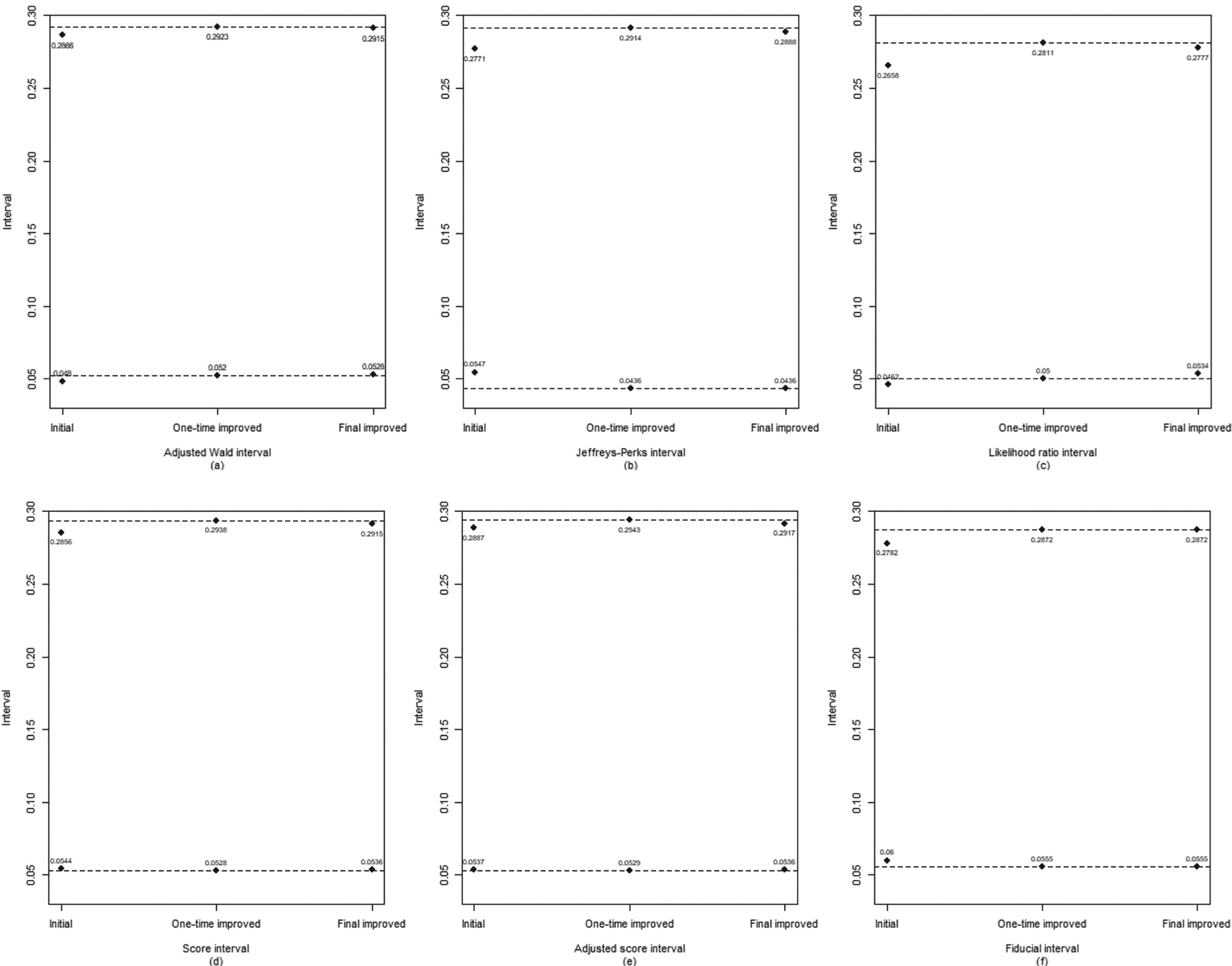
In order to observe the changes of intervals at the fixed sample point $(x_{1}, n_{1}, x_{2}, n_{2}) = (4, 18, 1, 15)$ in the improvement process, we give the lower and upper limits of six given initial intervals, the one-time improved intervals, and the final improved intervals, respectively, as shown in Figure 1. It is evident that all final improved exact intervals are subsets of the corresponding one-time improved exact interval. Therefore, the $h$ -function method continuously shortens exact intervals and the final improved intervals depend on the initial intervals.

Figure 1.

Six initial 95% approximate intervals and their one-time and final improved exact intervals at $(x_{1}, n_{1}, x_{2}, n_{2}) = (4, 18, 1, 15)$ in Example 1. The dot points are the lower and upper limits of intervals, and the dashed lines represent the lower and upper limits of the one-time improved exact interval.

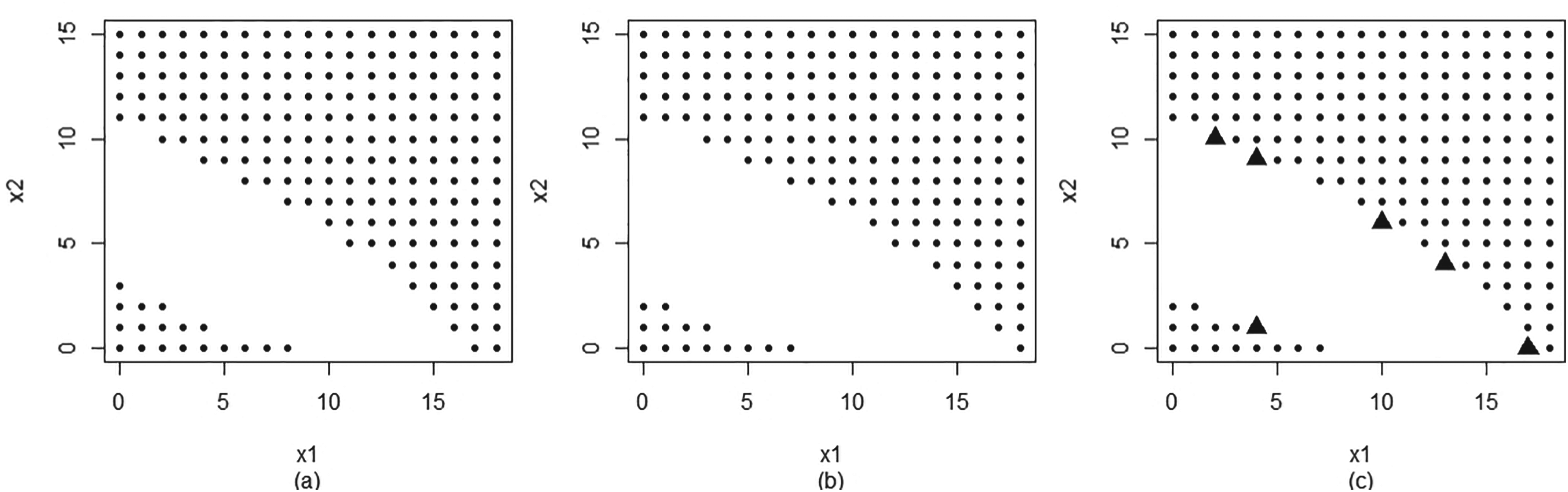
Figure 2 exhibits three level-0.05 rejection regions of the likelihood-ratio test, the one-time improved $T_{C}$ test and the final improved $T_{C}$ test, respectively, for the hypotheses in (12) when $η_{0} = 0.278$ and $(n_{1}, n_{2}) = (18, 15)$ . The rejection region of the final improved $T_{C}$ test is the union of that of the one-time improved $T_{C}$ test and six triangle points. In particular, the observed sample point $(x_{1}, x_{2}) = (4, 1)$ in Example 1 belongs to the former region but not the latter region. So, the final improved $T_{C}$ test is uniformly more powerful than the one-time improved $T_{C}$ test, and this conclusion is consistent with the fact that the final improved interval $C_{η}^{I F}$ is contained in the one-time improved interval $C_{η}^{I}$ .

Figure 2.

Three level-0.05 rejection regions for testing $H_{0} : η = 0.278$ in Example 1 when $(n_{1}, n_{2}) = (18, 15)$ : (a) the likelihood ratio test (the dots); (b) the one-time improved test (the dots); and (c) the final improved test (the dots plus the triangles).

3.3. Comparing the six approximate intervals and their exact improvements

We evaluate the performance of a confidence interval using the ICP for reliability and the total interval length (TIL) for precision. For a given interval $C_{λ} (\underline{X}) = [L_{λ} (\underline{X}), U_{λ} (\underline{X})]$ of $λ$ , its coverage probability function is

C o v e r_{C_{λ}} (p_{1}, \dots, p_{k}) = \sum_{x_{1} = 0}^{n_{1}} \dots \sum_{x_{k} = 0}^{n_{k}} [I (L_{λ} (\underline{x}) \leq λ \leq U_{λ} (\underline{x})) \prod_{i = 1}^{k} p_{B} (x_{i}; n_{i}, p_{i})]

(15)

Then, the ICP of interval

C_{λ}

is the infimum of

C o v e r_{C_{λ}} (p_{1}, \dots, p_{k})

over the entire parameter space

H

. The TIL of interval

C_{λ}

T I L (C_{λ}) = \sum_{\underline{x} \in S} [U_{λ} (\underline{x}) - L_{λ} (\underline{x})]

(16)

which is well-defined due to the finite sample space

S

and the finite range of

λ

. The TIL is a much simpler measurement for precision than the expected length of

C_{λ}

since the TIL is a single value but the expected length is a function of the parameter vector

(p_{1}, \dots, p_{k})

and comparing two single values is much easier than comparing two functions. A good exact interval

C_{λ}

should have an ICP no less than

1 - α

and a small TIL. In particular, for two exact intervals

C_{λ 1}

and

C_{λ 2}

C_{λ 1}

is preferred if

T I L (C_{λ 1}) < T I L (C_{λ 2})

In Section 3.1, we obtain 18 confidence intervals for $η$ , including six original (approximate) intervals $C_{η j}$ , six one-time improved (exact) intervals $C_{η j}^{I}$ , and six final-improved (exact) intervals $C_{η j}^{I F}$ for $j = 1, \dots, 6$ . Wang¹⁴ ensured that the shortest exact interval here should be equal to one of the $C_{η j}^{I F}$ ’s.

When using the $h$ -function method to improve an interval, numerical calculation errors may occur in the interval construction process, especially when implementing (10) and (11). Equation (10) computes a global supremum of probability over $H_{0}$ and equation (11) solves the smallest and largest roots of the $h$ -function larger than $α$ . No existing software is able to find these values quickly and always correctly because a software typically provides a local supremum and an arbitrary root. Therefore, calculating the ICP of improved intervals is an effective way to validate the computation of the intervals. If the calculated ICP is not smaller than $1 - α$ , it is safe to say that the improved interval is correct. Otherwise, there exist some errors in the computation.

We can compute the coverage probability of any $C_{η}$ at any given point $(p_{1}, p_{2})$ in $H_{1}$ using (15) without any errors. However, since the coverage probability function is not continuous, the ICP requires extensive computations: (i) choose 140,000 of pairs $(p_{1}, p_{2})$ in the parameter space $H_{1}$ . Among them, 40,000 pairs are selected in a way that each $p_{i}$ is equal to the multiples of 0.005, and 100,000 pairs are randomly selected from $H_{1}$ . (ii) Compute the precise coverage probabilities at these pairs using (15) and the minimum of these coverage probabilities is the computed ICP.

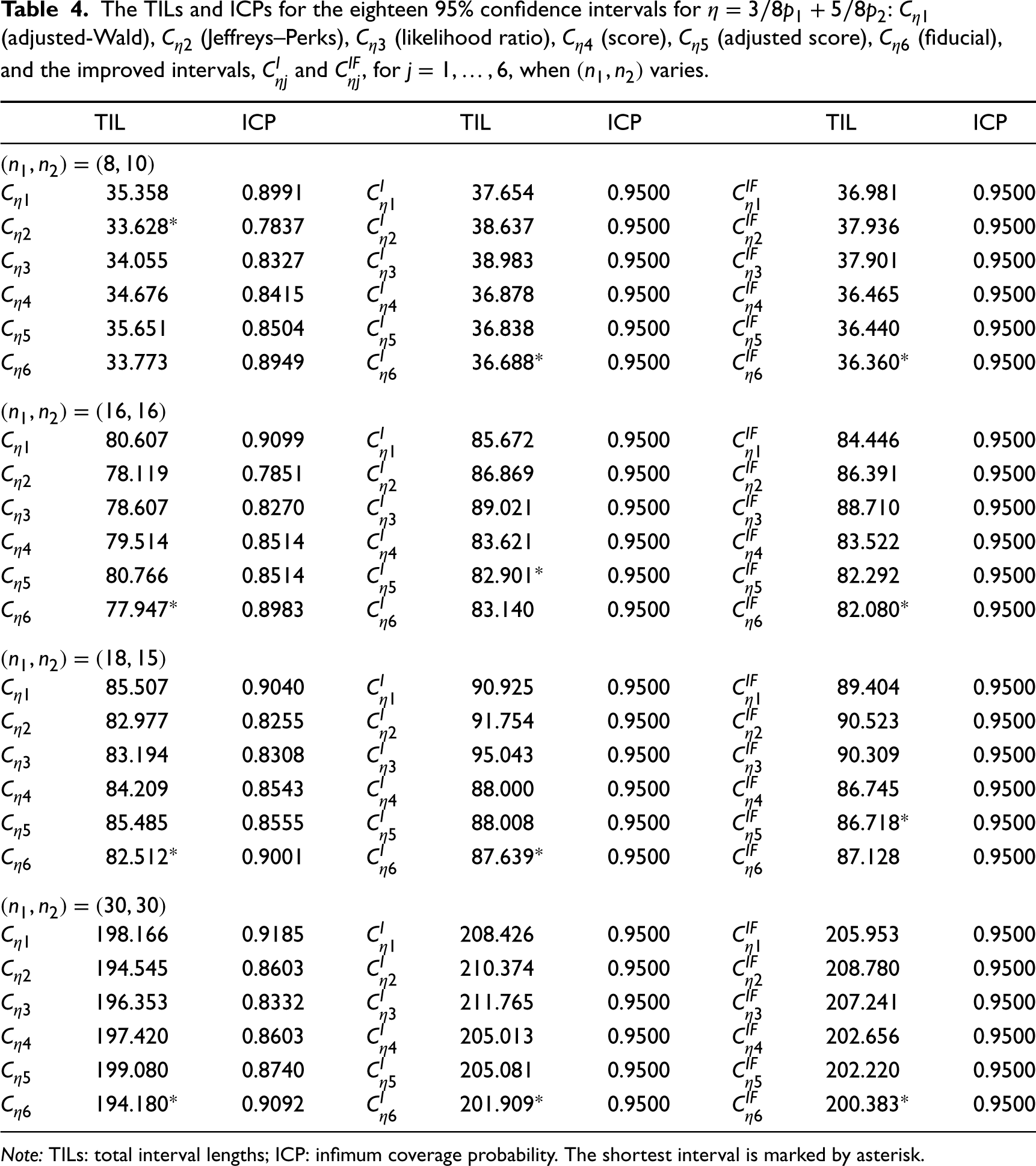
Table 4 contains the TIL and ICP of the eighteen 95% intervals discussed so far for four cases of $(n_{1}, n_{2})$ . Decrouez and Robinson¹³ claimed the adjusted score interval $C_{η 5}$ is the best for small samples. However, we find the ICP of $C_{η 5}$ is worse than those of $C_{η 1}$ and $C_{η 6}$ . Interestingly, $C_{η 6}$ also has a smaller TIL than $C_{η 5}$ . So, $C_{η 6}$ is better than $C_{η 5}$ because the former has a larger ICP but a smaller TIL. Nevertheless, none of these approximate intervals reach the nominal level 0.95, while all the improved intervals $C_{η j}^{I}$ and $C_{η j}^{I F}$ have an ICP at 0.95. We find that $C_{η 6}^{I F}$ or $C_{η 5}^{I F}$ is the shortest among the exact intervals. If the computation time is a concern, one may use the one-time improved interval $C_{η 6}^{I}$ or $C_{η 5}^{I}$ .

Table 4.

The TILs and ICPs for the eighteen 95% confidence intervals for $η = 3 / 8 p_{1} + 5 / 8 p_{2}$ : $C_{η 1}$ (adjusted-Wald), $C_{η 2}$ (Jeffreys–Perks), $C_{η 3}$ (likelihood ratio), $C_{η 4}$ (score), $C_{η 5}$ (adjusted score), $C_{η 6}$ (fiducial), and the improved intervals, $C_{η j}^{I}$ and $C_{η j}^{I F}$ , for $j = 1, \dots, 6$ , when $(n_{1}, n_{2})$ varies.

	TIL	ICP		TIL	ICP		TIL	ICP
$(n_{1}, n_{2}) = (8, 10)$
$C_{η 1}$	35.358	0.8991	$C_{η 1}^{I}$	37.654	0.9500	$C_{η 1}^{I F}$	36.981	0.9500
$C_{η 2}$	33.628*	0.7837	$C_{η 2}^{I}$	38.637	0.9500	$C_{η 2}^{I F}$	37.936	0.9500
$C_{η 3}$	34.055	0.8327	$C_{η 3}^{I}$	38.983	0.9500	$C_{η 3}^{I F}$	37.901	0.9500
$C_{η 4}$	34.676	0.8415	$C_{η 4}^{I}$	36.878	0.9500	$C_{η 4}^{I F}$	36.465	0.9500
$C_{η 5}$	35.651	0.8504	$C_{η 5}^{I}$	36.838	0.9500	$C_{η 5}^{I F}$	36.440	0.9500
$C_{η 6}$	33.773	0.8949	$C_{η 6}^{I}$	36.688*	0.9500	$C_{η 6}^{I F}$	36.360*	0.9500
$(n_{1}, n_{2}) = (16, 16)$
$C_{η 1}$	80.607	0.9099	$C_{η 1}^{I}$	85.672	0.9500	$C_{η 1}^{I F}$	84.446	0.9500
$C_{η 2}$	78.119	0.7851	$C_{η 2}^{I}$	86.869	0.9500	$C_{η 2}^{I F}$	86.391	0.9500
$C_{η 3}$	78.607	0.8270	$C_{η 3}^{I}$	89.021	0.9500	$C_{η 3}^{I F}$	88.710	0.9500
$C_{η 4}$	79.514	0.8514	$C_{η 4}^{I}$	83.621	0.9500	$C_{η 4}^{I F}$	83.522	0.9500
$C_{η 5}$	80.766	0.8514	$C_{η 5}^{I}$	82.901*	0.9500	$C_{η 5}^{I F}$	82.292	0.9500
$C_{η 6}$	77.947*	0.8983	$C_{η 6}^{I}$	83.140	0.9500	$C_{η 6}^{I F}$	82.080*	0.9500
$(n_{1}, n_{2}) = (18, 15)$
$C_{η 1}$	85.507	0.9040	$C_{η 1}^{I}$	90.925	0.9500	$C_{η 1}^{I F}$	89.404	0.9500
$C_{η 2}$	82.977	0.8255	$C_{η 2}^{I}$	91.754	0.9500	$C_{η 2}^{I F}$	90.523	0.9500
$C_{η 3}$	83.194	0.8308	$C_{η 3}^{I}$	95.043	0.9500	$C_{η 3}^{I F}$	90.309	0.9500
$C_{η 4}$	84.209	0.8543	$C_{η 4}^{I}$	88.000	0.9500	$C_{η 4}^{I F}$	86.745	0.9500
$C_{η 5}$	85.485	0.8555	$C_{η 5}^{I}$	88.008	0.9500	$C_{η 5}^{I F}$	86.718*	0.9500
$C_{η 6}$	82.512*	0.9001	$C_{η 6}^{I}$	87.639*	0.9500	$C_{η 6}^{I F}$	87.128	0.9500
$(n_{1}, n_{2}) = (30, 30)$
$C_{η 1}$	198.166	0.9185	$C_{η 1}^{I}$	208.426	0.9500	$C_{η 1}^{I F}$	205.953	0.9500
$C_{η 2}$	194.545	0.8603	$C_{η 2}^{I}$	210.374	0.9500	$C_{η 2}^{I F}$	208.780	0.9500
$C_{η 3}$	196.353	0.8332	$C_{η 3}^{I}$	211.765	0.9500	$C_{η 3}^{I F}$	207.241	0.9500
$C_{η 4}$	197.420	0.8603	$C_{η 4}^{I}$	205.013	0.9500	$C_{η 4}^{I F}$	202.656	0.9500
$C_{η 5}$	199.080	0.8740	$C_{η 5}^{I}$	205.081	0.9500	$C_{η 5}^{I F}$	202.220	0.9500
$C_{η 6}$	194.180*	0.9092	$C_{η 6}^{I}$	201.909*	0.9500	$C_{η 6}^{I F}$	200.383*	0.9500

Note: TILs: total interval lengths; ICP: infimum coverage probability. The shortest interval is marked by asterisk.

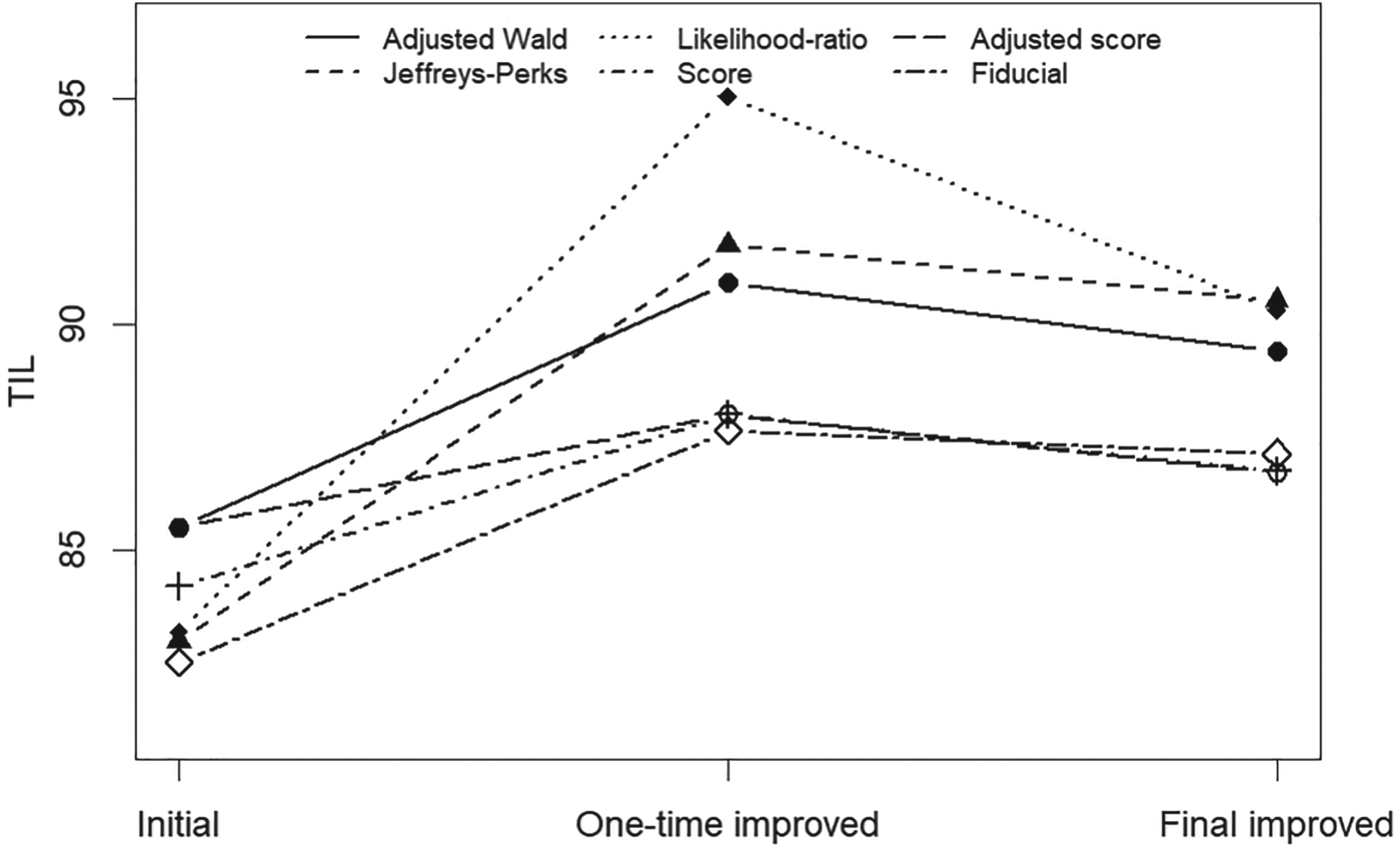
To gain insight into the overall changes in confidence intervals, we present the TILs of six given initial intervals, the one-time improved intervals, and the final improved intervals in Figure 3. Notably, the TILs of all final improved exact intervals are shorter than those of the corresponding one-time improved exact intervals. This observation underscores the effectiveness of the $h$ -function method in continuously shortening exact intervals. Again, different initial intervals lead to different final improved intervals. Here, the final improved adjusted score interval $C_{η 5}^{I}$ is the shortest.

Figure 3.

The total interval lengths (TILs) of eighteen 95% confidence intervals for $η$ when $(n_{1}, n_{2}) = (18, 15)$ .

4. Exact intervals for the weighted sum of three proportions

We now consider the weighted sum of proportions for $k = 3$ . Three independent $X_{i} \sim B i n o (n_{i}, p_{i})$ ’s for $i = 1, 2, 3$ are observed. The parameter and sample spaces are

H_{2} = {(p_{1}, p_{2}, p_{3}) : 0 \leq p_{1}, p_{2}, p_{3} \leq 1} and S_{2} = {(x_{1}, x_{2}, x_{3}) : x_{i} \in [0, n_{i}], i = 1, 2, 3}

respectively. The parameter of interest is

ξ = c_{1} p_{1} + c_{2} p_{2} + c_{3} p_{3}

, for some

c_{i} > 0

and

c_{1} + c_{2} + c_{3} = 1

, and the range of

ξ

is still

[0, 1]

For any fixed $ξ_{0} \in [0, 1]$ , consider the hypotheses:

H_{0} : ξ = ξ_{0} versus H_{A} : ξ \neq ξ_{0}

The null hypothesis, in terms of

(p_{1}, p_{2}, p_{3})

, is equal to

{(p_{1} (p_{2}, p_{3}, ξ_{0}), p_{2}, p_{3}) : p_{2} \in D (ξ_{0}), p_{3} \in D (p_{2}, ξ_{0})},

where

p_{1} (p_{2}, p_{3}, ξ_{0}) = (ξ_{0} - c_{2} p_{2} - c_{3} p_{3}) / c_{1},

D (ξ_{0}) = [max {\frac{ξ_{0} - c_{1} - c_{3}}{c_{2}}, 0}, min {\frac{ξ_{0}}{c_{2}}, 1}]

and

D (p_{2}, ξ_{0}) = [max {\frac{ξ_{0} - c_{2} p_{2} - c_{1}}{c_{3}}, 0}, min {\frac{ξ_{0} - c_{2} p_{2}}{c_{3}}, 1}]

Similar to Section 3, for a given interval

C_{ξ} (X_{1}, X_{2}, X_{3}) = [L_{ξ} (X_{1}, X_{2}, X_{3}), U_{ξ} (X_{1}, X_{2}, X_{3})]

for

ξ

, introduce the test statistic and

h

-function below follow (9) and (10):

T_{ξ} (X_{1}, X_{2}, X_{3}, ξ_{0}) = min {ξ_{0} - L_{ξ} (X_{1}, X_{2}, X_{3}), U_{ξ} (X_{1}, X_{2}, X_{3}) - ξ_{0}}

and

h_{ξ} (x_{1}, x_{2}, x_{3}, ξ_{0}) = sup_{p_{2} \in D (ξ_{0}), p_{3} \in D (p_{2}, ξ_{0})} \sum_{S (x_{1}, x_{2}, x_{3})} p_{B} (u; n_{1}, p_{1}) p_{B} (v; n_{2}, p_{2}) p_{B} (z; n_{3}, p_{3})

where

S (x_{1}, x_{2}, x_{3}) = {(u, v, z) \in S_{2} : T_{ξ} (u, v, z, ξ_{0}) \leq T_{ξ} (x_{1}, x_{2}, x_{3}, ξ_{0})}

. Then, the one-time improved confidence interval for

ξ

(x_{1}, x_{2}, x_{3})

C_{ξ}^{I} (x_{1}, x_{2}, x_{3}) = [L_{ξ}^{I} (x_{1}, x_{2}, x_{3}), U_{ξ}^{I} (x_{1}, x_{2}, x_{3})],

where

L_{ξ}^{I} (x_{1}, x_{2}, x_{3})

and

U_{ξ}^{I} (x_{1}, x_{2}, x_{3})

are the infimum and supremum of set

{ξ_{0} : h_{ξ} (x_{1}, x_{2}, x_{3}, ξ_{0}) > α}

, respectively. Furthermore, we derive the final-improved interval

C_{ξ}^{I F} (X_{1}, X_{2}, X_{3})

, a subset of

C_{ξ}^{I} (X_{1}, X_{2}, X_{3})

4.1. Improving five approximate intervals to exact intervals

We use the above procedure to improve the following five approximate intervals to exact intervals and then uniformly shorten these exact intervals.

The five approximate intervals, $C_{ξ j}$ for $j = 1, \dots, 5$ , are the special cases of the adjusted Wald interval $C_{W a}$ in (3), the modified Wilson interval $C_{W i}$ in (4), the score interval $C_{S}$ in (6), the adjusted score interval $C_{A S}$ in (7), and the fiducial interval $C_{F}$ in (8), respectively, for $k = 3$ . After applying the $h$ -function method to these approximate intervals, we obtain the one-time improved intervals $C_{ξ j}^{I}$ and the final-improved intervals $C_{ξ j}^{I F}$ for $j = 1, \dots, 5$ .

4.2. Interval comparison and a real-data analysis

The comparison among $1 - α$ intervals is still conducted using the ICP in (15) for reliability and the TIL in (16) for precision.

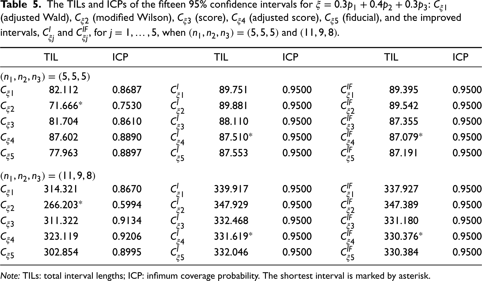
The TIL and ICP of the five approximate 95% intervals and 10 exact improved intervals discussed in the previous section are presented in Table 5. Zou et al. claimed that the modified Wilson interval $C_{ξ 2}$ is shorter than the adjusted Wald interval $C_{ξ 1}$ . This is true in the table, but we also find $C_{ξ 2}$ has a much smaller ICP than $C_{ξ 1}$ . In other words, the dominance of $C_{ξ 2}$ over $C_{ξ 1}$ on TIL is because it has an ICP value 0.7530 much less than both of 0.95, the nominal level, and 0.8687, the ICP of $C_{ξ 1}$ . In fact, if we only compare the TIL, $C_{ξ 2}$ would be the best interval among the five approximate intervals in Table 5. Again, this is because $C_{ξ 2}$ has the smallest ICP’s (0.7530 and 0.5994). It is not appropriate to conclude that $C_{ξ 2}$ is the shortest interval without checking the ICP.

Any comparison, including interval comparison, must have an objective baseline. The above discussion shows that the nominal level $1 - α$ does not serve this purpose. The major problem is that an interval of level $1 - α$ may have an ICP value anywhere in $[0, 1]$ . An example is the well-known Wald interval for a single proportion that has a zero ICP for any sample size, see Agresti.¹⁸ However, it is also a common practice to compare intervals which have the same nominal level $1 - α$ . In particular, this occurs frequently in comparison of approximate intervals. Such practices are easy to implement but often lead to some misleading conclusions, including that $C_{ξ 2}$ is the shortest.

Table 5.
The TILs and ICPs of the fifteen 95% confidence intervals for $ξ = 0.3 p_{1} + 0.4 p_{2} + 0.3 p_{3}$ : $C_{ξ 1}$ (adjusted Wald), $C_{ξ 2}$ (modified Wilson), $C_{ξ 3}$ (score), $C_{ξ 4}$ (adjusted score), $C_{ξ 5}$ (fiducial), and the improved intervals, $C_{ξ j}^{I}$ and $C_{ξ j}^{I F}$ , for $j = 1, \dots, 5$ , when $(n_{1}, n_{2}, n_{3}) = (5, 5, 5)$ and $(11, 9, 8)$ .

TIL ICP TIL ICP TIL ICP

$(n_{1}, n_{2}, n_{3}) = (5, 5, 5)$

$C_{ξ 1}$ 82.112 0.8687 $C_{ξ 1}^{I}$ 89.751 0.9500 $C_{ξ 1}^{I F}$ 89.395 0.9500

$C_{ξ 2}$ 71.666* 0.7530 $C_{ξ 2}^{I}$ 89.881 0.9500 $C_{ξ 2}^{I F}$ 89.542 0.9500

$C_{ξ 3}$ 81.704 0.8610 $C_{ξ 3}^{I}$ 88.110 0.9500 $C_{ξ 3}^{I F}$ 87.355 0.9500

$C_{ξ 4}$ 87.602 0.8890 $C_{ξ 4}^{I}$ 87.510* 0.9500 $C_{ξ 4}^{I F}$ 87.079* 0.9500

$C_{ξ 5}$ 77.963 0.8897 $C_{ξ 5}^{I}$ 87.553 0.9500 $C_{ξ 5}^{I F}$ 87.191 0.9500

$(n_{1}, n_{2}, n_{3}) = (11, 9, 8)$

$C_{ξ 1}$ 314.321 0.8670 $C_{ξ 1}^{I}$ 339.917 0.9500 $C_{ξ 1}^{I F}$ 337.927 0.9500

$C_{ξ 2}$ 266.203* 0.5994 $C_{ξ 2}^{I}$ 347.929 0.9500 $C_{ξ 2}^{I F}$ 347.389 0.9500

$C_{ξ 3}$ 311.322 0.9134 $C_{ξ 3}^{I}$ 332.468 0.9500 $C_{ξ 3}^{I F}$ 331.180 0.9500

$C_{ξ 4}$ 323.119 0.9206 $C_{ξ 4}^{I}$ 331.619* 0.9500 $C_{ξ 4}^{I F}$ 330.376* 0.9500

$C_{ξ 5}$ 302.854 0.8995 $C_{ξ 5}^{I}$ 332.046 0.9500 $C_{ξ 5}^{I F}$ 330.384 0.9500

	TIL	ICP		TIL	ICP		TIL	ICP
$(n_{1}, n_{2}, n_{3}) = (5, 5, 5)$
$C_{ξ 1}$	82.112	0.8687	$C_{ξ 1}^{I}$	89.751	0.9500	$C_{ξ 1}^{I F}$	89.395	0.9500
$C_{ξ 2}$	71.666*	0.7530	$C_{ξ 2}^{I}$	89.881	0.9500	$C_{ξ 2}^{I F}$	89.542	0.9500
$C_{ξ 3}$	81.704	0.8610	$C_{ξ 3}^{I}$	88.110	0.9500	$C_{ξ 3}^{I F}$	87.355	0.9500
$C_{ξ 4}$	87.602	0.8890	$C_{ξ 4}^{I}$	87.510*	0.9500	$C_{ξ 4}^{I F}$	87.079*	0.9500
$C_{ξ 5}$	77.963	0.8897	$C_{ξ 5}^{I}$	87.553	0.9500	$C_{ξ 5}^{I F}$	87.191	0.9500
$(n_{1}, n_{2}, n_{3}) = (11, 9, 8)$
$C_{ξ 1}$	314.321	0.8670	$C_{ξ 1}^{I}$	339.917	0.9500	$C_{ξ 1}^{I F}$	337.927	0.9500
$C_{ξ 2}$	266.203*	0.5994	$C_{ξ 2}^{I}$	347.929	0.9500	$C_{ξ 2}^{I F}$	347.389	0.9500
$C_{ξ 3}$	311.322	0.9134	$C_{ξ 3}^{I}$	332.468	0.9500	$C_{ξ 3}^{I F}$	331.180	0.9500
$C_{ξ 4}$	323.119	0.9206	$C_{ξ 4}^{I}$	331.619*	0.9500	$C_{ξ 4}^{I F}$	330.376*	0.9500
$C_{ξ 5}$	302.854	0.8995	$C_{ξ 5}^{I}$	332.046	0.9500	$C_{ξ 5}^{I F}$	330.384	0.9500

Note: TILs: total interval lengths; ICP: infimum coverage probability. The shortest interval is marked by asterisk.

A fair baseline for interval comparison is to require an ICP not less than the nominal level $1 - α$ , that is, we choose an interval with the shortest TIL as the best interval among exact intervals. Using the TIL rather than the expected length makes such a choice possible because the TIL is a single value, but the expected length is a function over the parameter space and the interval with the smallest expected length typically does not exist. Table 5 shows that $C_{ξ 4}^{I F}$ is the shortest. So, when $k = 3$ we recommend the final-improved adjusted score interval $C_{ξ 4}^{I F}$ or the one-time improved interval $C_{ξ 4}^{I}$ if the computation time for $C_{ξ 4}^{I F}$ is a big concern. Martín Andr $\overset{´}{e}$ s et al. recommended the score interval $C_{ξ 3}$ and the Wald3 interval, a variant of the Wald interval. The final-improved interval for the Wald3 interval has a large TIL, and we do not include the numerical results of this interval.

Example 3

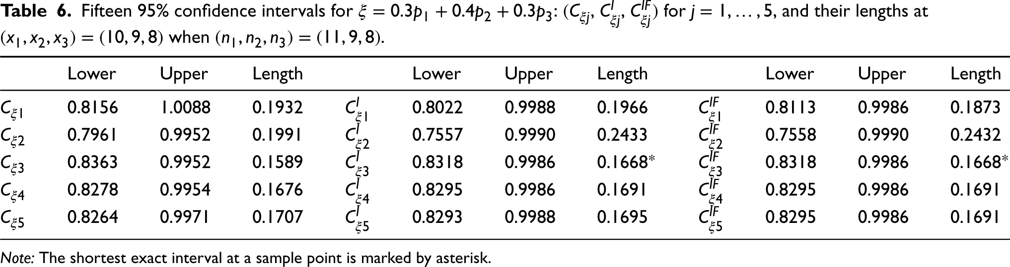
Li et al.¹⁹ conducted a study on the efficacy of thymosin in the treatment of bronchogenic carcinoma patients receiving radiotherapy in three gruops

(k = 3)

. The sample sizes and the number of survival for the three groups are

(x_{1}, n_{1}, x_{2}, n_{2}, x_{3}, n_{3}) = (10, 11, 9, 9, 8, 8)

. Let

p_{1}

p_{2}

and

p_{3}

be the survival rates for the three groups, respectively. Our goal is to estimate the overall survival rate of patients under the assumption that the ratio of three groups is

3 : 4 : 3

. Then, the parameter of interest is

ξ = c_{1} p_{1} + c_{2} p_{2} + c_{3} p_{3}

for

c_{1} = 0.3, c_{2} = 0.4

, and

c_{3} = 0.3

. Fifteen intervals and their lengths at the observed point

(x_{1}, x_{2}, x_{3}) = (10, 9, 8)

are listed in Table 6. The final-improved score interval

C_{ξ 3}^{I F} (10, 9, 8) = [0.8318, 0.9986]

is the shortest.

Table 6.

Fifteen 95% confidence intervals for $ξ = 0.3 p_{1} + 0.4 p_{2} + 0.3 p_{3}$ : $(C_{ξ j}$ , $C_{ξ j}^{I}$ , $C_{ξ j}^{I F})$ for $j = 1, \dots, 5$ , and their lengths at $(x_{1}, x_{2}, x_{3}) = (10, 9, 8)$ when $(n_{1}, n_{2}, n_{3}) = (11, 9, 8)$ .

	Lower	Upper	Length		Lower	Upper	Length		Lower	Upper	Length
$C_{ξ 1}$	0.8156	1.0088	0.1932	$C_{ξ 1}^{I}$	0.8022	0.9988	0.1966	$C_{ξ 1}^{I F}$	0.8113	0.9986	0.1873
$C_{ξ 2}$	0.7961	0.9952	0.1991	$C_{ξ 2}^{I}$	0.7557	0.9990	0.2433	$C_{ξ 2}^{I F}$	0.7558	0.9990	0.2432
$C_{ξ 3}$	0.8363	0.9952	0.1589	$C_{ξ 3}^{I}$	0.8318	0.9986	0.1668^*	$C_{ξ 3}^{I F}$	0.8318	0.9986	0.1668^*
$C_{ξ 4}$	0.8278	0.9954	0.1676	$C_{ξ 4}^{I}$	0.8295	0.9986	0.1691	$C_{ξ 4}^{I F}$	0.8295	0.9986	0.1691
$C_{ξ 5}$	0.8264	0.9971	0.1707	$C_{ξ 5}^{I}$	0.8293	0.9988	0.1695	$C_{ξ 5}^{I F}$	0.8295	0.9986	0.1691

Note: The shortest exact interval at a sample point is marked by asterisk.

5. Exact intervals for the interaction effect

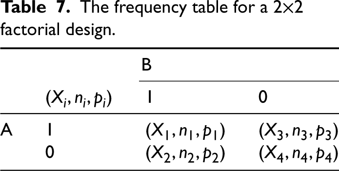
We assess the interaction effect in a two-factor factorial design of two factors A and B, where each factor assumes two levels: 1 and 0. Suppose four independent binomials are observed from the factor-level combinations: $X_{i} \sim B i n o (n_{i}, p_{i})$ , $i = 1, 2, 3, 4$ as shown in Table 7.

Table 7.
The frequency table for a 2 $\times$ 2 factorial design.

B

( $X_{i}, n_{i}, p_{i}$ ) 1 0

A 1 ( $X_{1}, n_{1}, p_{1}$ ) ( $X_{3}, n_{3}, p_{3}$ )

0 ( $X_{2}, n_{2}, p_{2}$ ) ( $X_{4}, n_{4}, p_{4}$ )

		B
A	1	( $X_{1}, n_{1}, p_{1}$ )	( $X_{3}, n_{3}, p_{3}$ )
	0	( $X_{2}, n_{2}, p_{2}$ )	( $X_{4}, n_{4}, p_{4}$ )

The parameter of interest is the interaction effect, measured by $θ = (p_{1} - p_{2}) - (p_{3} - p_{4})$ with a range of $[- 2, 2]$ . Similar to the analysis of variance, when $θ$ is not equal to zero, then there exists an interaction effect between factors A and B.

Denote the parameter and sample spaces by

H_{3} = {(p_{1}, p_{2}, p_{3}, p_{4}) : 0 \leq p_{1}, p_{2}, p_{3}, p_{4} \leq 1} and S_{3} = {(x_{1}, x_{2}, x_{3}, x_{4}) : x_{i} \in [0, n_{i}], i = 1, 2, 3, 4}

respectively. For any fixed

θ_{0} \in [- 2, 2]

, consider the hypotheses:

H_{0} : θ = θ_{0} versus H_{A} : θ \neq θ_{0}

The null hypothesis is rewritten as

H_{0} = {(p_{1} (p_{2}, p_{3}, p_{4}, θ_{0}), p_{2}, p_{3}, p_{4}) : p_{4} \in D (θ_{0}), p_{3} \in D (p_{4}, θ_{0}), p_{2} \in D (p_{3}, p_{4}, θ_{0})}

where

p_{1} (p_{2}, p_{3}, p_{4}, θ_{0}) = θ_{0} + p_{2} + p_{3} - p_{4},

\begin{aligned} D (θ_{0}) = [max {θ_{0} - 1, 0}, min {θ_{0} + 2, 1}] \\ D (p_{4}, θ_{0}) = [max {- θ_{0} + p_{4} - 1, 0}, min {- θ_{0} + p_{4} + 1, 1}] \\ D (p_{3}, p_{4}, θ_{0}) = [max {- (θ_{0} + p_{3} - p_{4}), 0}, min {1 - (θ_{0} + p_{3} - p_{4}), 1}] \end{aligned}

As described in Section 2, for any given interval

C_{θ}

for

θ

, we follow the process of (9) to (11) and derive the one-time and final-improved intervals

C_{θ}^{I}

and

C_{θ}^{I F}

, respectively.

We improve the five approximate intervals discussed in Section 2.1 for the interaction effect $θ$ , that is, the adjusted Wald interval $C_{θ 1}$ , the modified Wilson interval $C_{θ 2}$ , the score interval $C_{θ 3}$ , the adjusted score interval $C_{θ 4}$ , and the fiducial interval $C_{θ 5}$ . These intervals are given in (3), (4), and (6) to (8), respectively, using $k = 4$ , $c_{1} = c_{4} = 1$ , and $c_{2} = c_{3} = - 1$ . Also, their exact improvements $C_{θ j}^{I}$ and $C_{θ j}^{I F}$ for $j = 1, \dots, 5$ are derived.

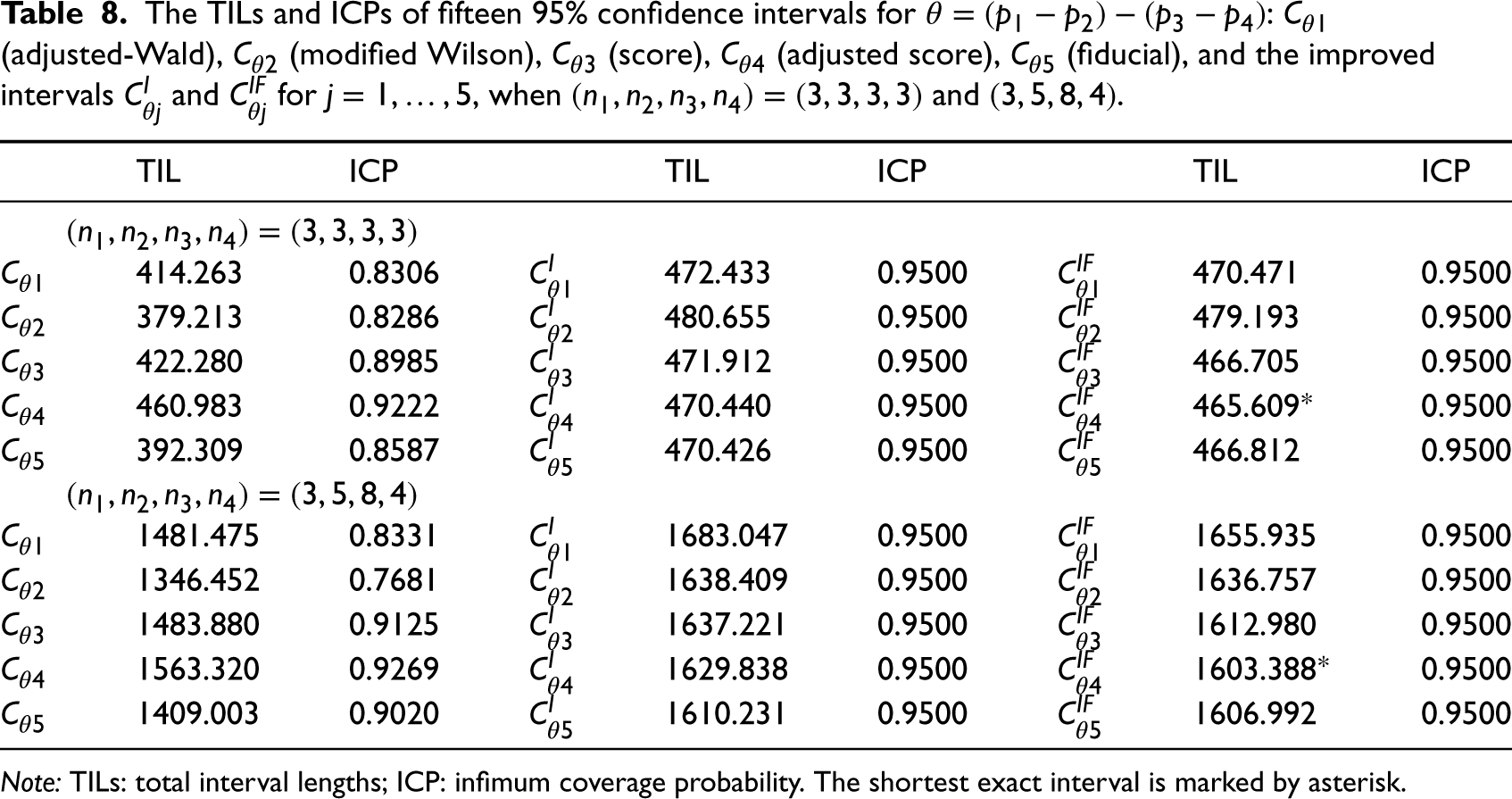
The TIL and ICP of these 95% intervals are displayed in Table 8 for two cases of small sample sizes. The final-improved adjusted score interval $C_{θ 4}^{I F}$ is shorter than the others.

Example 2 (continued). The dataset in Table 2 yields $n_{1} = n_{2} = n_{3} = n_{4} = 10$ and $(x_{1}, x_{2}, x_{3}, x_{4}) = (8, 9, 5, 10)$ in the setting of Table 7. Here, $x_{i}$ is the number of persons who recalled more than six words for a factor-level combination and $p_{i}$ is the success probability of the binomial $X_{i}$ . The parameter of interest is the interaction effect,

θ = (p_{1} - p_{2}) - (p_{3} - p_{4})

(17)

At the observed

(8, 9, 5, 10)

, the five one-time improved intervals are

C_{θ 1}^{I} = [- 0.1181, 0.8682]

C_{θ 2}^{I} = [- 0.1635, 0.8655]

C_{θ 3}^{I} = [- 0.0802, 0.8822]

C_{θ 4}^{I} = [- 0.0799, 0.8768]

, and

C_{θ 5}^{I} = [- 0.1036, 0.8753]

, and their lengths are 0.9863, 1.0290, 0.9624, 0.9567, and 0.9789, respectively. Here,

C_{θ 4}^{I}

is the shortest. All intervals include zero. Hence, there is no significant interaction effect. Due to the computation time, we do not compute the final-improved interval

C_{θ}^{I F}

here.

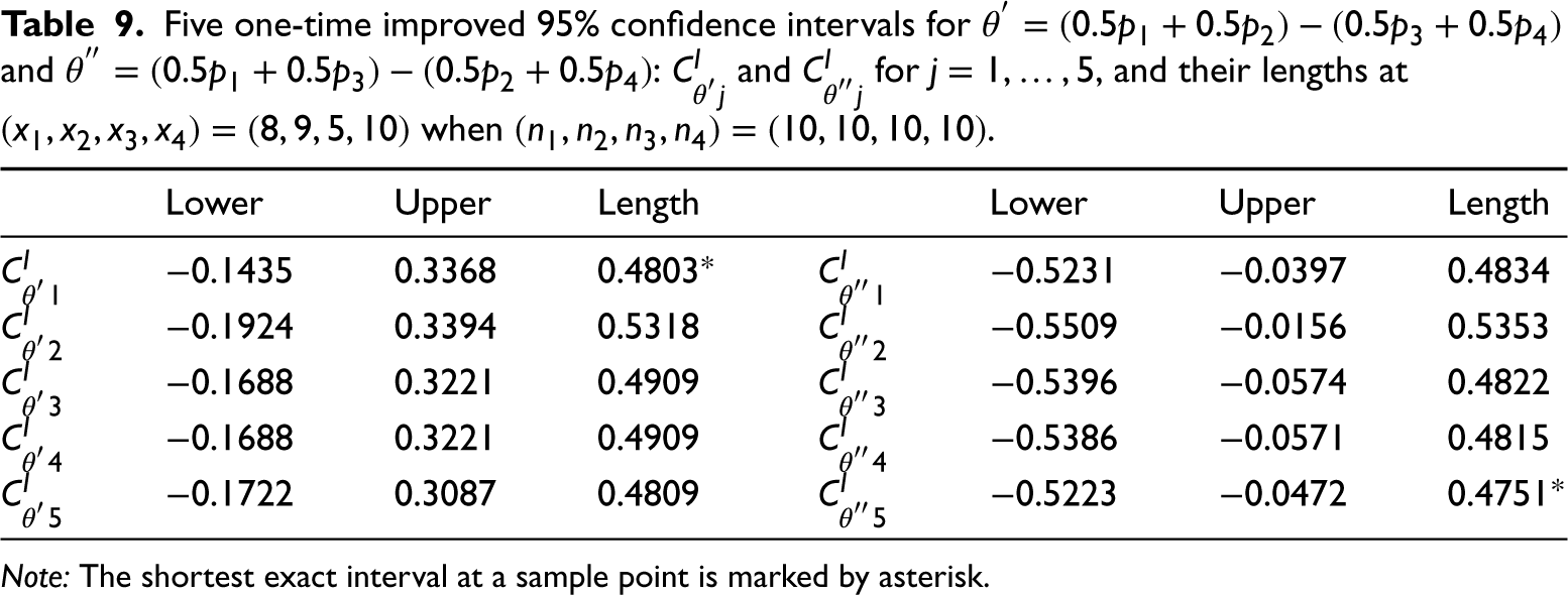
Similar to the two-way ANOVA, when there is no interaction, we estimate the two main effects: $θ^{'} = (0.5 p_{1} + 0.5 p_{2}) - (0.5 p_{3} + 0.5 p_{4})$ (age) and $θ^{″} = (0.5 p_{1} + 0.5 p_{3}) - (0.5 p_{2} + 0.5 p_{4})$ (instruction). At the observed $(8, 9, 5, 10)$ , the five one-time improved intervals for $θ^{'}$ and $θ^{″}$ are listed in Table 9. All intervals for $θ^{'}$ contain zero. So, age does not affect the number of words recalled. However, all intervals for $θ^{″}$ exclude zero. Instruction affects the number of words recalled and the probability of recalling seven words or more for the level “intentional” is less than that of the level “counting.” Here, $C_{θ^{″} 5}^{I}$ is the shortest interval.

Table 8.

The TILs and ICPs of fifteen 95% confidence intervals for $θ = (p_{1} - p_{2}) - (p_{3} - p_{4})$ : $C_{θ 1}$ (adjusted-Wald), $C_{θ 2}$ (modified Wilson), $C_{θ 3}$ (score), $C_{θ 4}$ (adjusted score), $C_{θ 5}$ (fiducial), and the improved intervals $C_{θ j}^{I}$ and $C_{θ j}^{I F}$ for $j = 1, \dots, 5$ , when $(n_{1}, n_{2}, n_{3}, n_{4}) = (3, 3, 3, 3)$ and $(3, 5, 8, 4)$ .

	TIL	ICP		TIL	ICP		TIL	ICP
$(n_{1}, n_{2}, n_{3}, n_{4}) = (3, 3, 3, 3)$
$C_{θ 1}$	414.263	0.8306	$C_{θ 1}^{I}$	472.433	0.9500	$C_{θ 1}^{I F}$	470.471	0.9500
$C_{θ 2}$	379.213	0.8286	$C_{θ 2}^{I}$	480.655	0.9500	$C_{θ 2}^{I F}$	479.193	0.9500
$C_{θ 3}$	422.280	0.8985	$C_{θ 3}^{I}$	471.912	0.9500	$C_{θ 3}^{I F}$	466.705	0.9500
$C_{θ 4}$	460.983	0.9222	$C_{θ 4}^{I}$	470.440	0.9500	$C_{θ 4}^{I F}$	465.609^*	0.9500
$C_{θ 5}$	392.309	0.8587	$C_{θ 5}^{I}$	470.426	0.9500	$C_{θ 5}^{I F}$	466.812	0.9500
$(n_{1}, n_{2}, n_{3}, n_{4}) = (3, 5, 8, 4)$
$C_{θ 1}$	1481.475	0.8331	$C_{θ 1}^{I}$	1683.047	0.9500	$C_{θ 1}^{I F}$	1655.935	0.9500
$C_{θ 2}$	1346.452	0.7681	$C_{θ 2}^{I}$	1638.409	0.9500	$C_{θ 2}^{I F}$	1636.757	0.9500
$C_{θ 3}$	1483.880	0.9125	$C_{θ 3}^{I}$	1637.221	0.9500	$C_{θ 3}^{I F}$	1612.980	0.9500
$C_{θ 4}$	1563.320	0.9269	$C_{θ 4}^{I}$	1629.838	0.9500	$C_{θ 4}^{I F}$	1603.388^*	0.9500
$C_{θ 5}$	1409.003	0.9020	$C_{θ 5}^{I}$	1610.231	0.9500	$C_{θ 5}^{I F}$	1606.992	0.9500

Note: TILs: total interval lengths; ICP: infimum coverage probability. The shortest exact interval is marked by asterisk.

Table 9.

Five one-time improved 95% confidence intervals for $θ^{'} = (0.5 p_{1} + 0.5 p_{2}) - (0.5 p_{3} + 0.5 p_{4})$ and $θ^{″} = (0.5 p_{1} + 0.5 p_{3}) - (0.5 p_{2} + 0.5 p_{4})$ : $C_{θ^{'} j}^{I}$ and $C_{θ^{″} j}^{I}$ for $j = 1, \dots, 5$ , and their lengths at $(x_{1}, x_{2}, x_{3}, x_{4}) = (8, 9, 5, 10)$ when $(n_{1}, n_{2}, n_{3}, n_{4}) = (10, 10, 10, 10)$ .

	Lower	Upper	Length		Lower	Upper	Length
$C_{θ^{'} 1}^{I}$	$-$ 0.1435	0.3368	0.4803^*	$C_{θ^{″} 1}^{I}$	$-$ 0.5231	$-$ 0.0397	0.4834
$C_{θ^{'} 2}^{I}$	$-$ 0.1924	0.3394	0.5318	$C_{θ^{″} 2}^{I}$	$-$ 0.5509	$-$ 0.0156	0.5353
$C_{θ^{'} 3}^{I}$	$-$ 0.1688	0.3221	0.4909	$C_{θ^{″} 3}^{I}$	$-$ 0.5396	$-$ 0.0574	0.4822
$C_{θ^{'} 4}^{I}$	$-$ 0.1688	0.3221	0.4909	$C_{θ^{″} 4}^{I}$	$-$ 0.5386	$-$ 0.0571	0.4815
$C_{θ^{'} 5}^{I}$	$-$ 0.1722	0.3087	0.4809	$C_{θ^{″} 5}^{I}$	$-$ 0.5223	$-$ 0.0472	0.4751^*

Note: The shortest exact interval at a sample point is marked by asterisk.

6. Discussion

The weighted sum of proportions and the interaction effect are two important cases of the general linear combination of proportions. How to estimate them with a guaranteed confidence? In this article, we first propose exact intervals to answer this question. We recommend the final-improved fiducial interval $C_{η 6}^{I F}$ or adjusted score interval $C_{η 5}^{I F}$ for the weighted sum of two proportions $η$ ; the final-improved adjusted score intervals $C_{ξ 4}^{I F}$ and $C_{θ 4}^{I F}$ for the weighted sum of three proportions $ξ$ and the interaction effect $θ$ , respectively. When the computation time is a concern, we use the one-time improved intervals.

There exist many approximate intervals for the weighted sum of proportions and interaction effect. However, as discussed in Section 4.2, simply selecting a seemingly short approximate interval, for example, $C_{ξ 2}$ , may result in a big loss on interval reliability. Thus, selecting a short interval without check its ICP should not be done in practice and utilizing exact intervals is necessary.

Exact intervals have a long-time reputation for being difficult to derive. With the appearance of the $h$ -function method, it is not a problem anymore at least from the mathematical point of view. This is because any interval can be improved to an exact interval following the process of (9) to (11). Furthermore, as the computing ability advances, the numerical implementations of exact intervals become more feasible.

One drawback for using the final-improved intervals is the computing time of these intervals. The major obstacle is from the calculation of $h_{C}$ in (10) as we still do not have an efficient computing program to find a global supremum quickly and precisely, especially for a multivariate function. As seen in Sections 3 to 5, we need to find the supremum of unary, binary, and ternary functions, respectively. In fact, this is a general optimization problem without a solid answer yet. A simple replacement for the final-improved interval is the one-time improved interval, which can be computed, as seen in Example 2, and also provides reliable inferences.

Supplemental Material

sj-pdf-1-smm-10.1177_09622802241229200 - Supplemental material for Exact interval estimation for the linear combination of binomial proportions

Supplemental material, sj-pdf-1-smm-10.1177_09622802241229200 for Exact interval estimation for the linear combination of binomial proportions by Shuiyun Lu, Weizhen Wang and Tianfa Xie in Statistical Methods in Medical Research

Footnotes

Declaration of conflicting interests

The author(s) declared no potential conflicts of interest with respect to the research, authorship, and/or publication of this article.

Funding

The author(s) disclosed receipt of the following financial support for the research, authorship, and/or publication of this article: Lu and Wang’s research is partially supported by the Beijing Natural Science Foundation (No. 1222002) and Xie’s research is partially supported by the National Natural Science Foundation of China (Nos. 11971045, 12071457).

ORCID iD

Weizhen Wang

Supplemental material

Supplemental material for this article is available online.

References

Innes

JRM

Ulland

Valerio

, et al. Bioassay of pesticides and industrial chemicals for tumorigenicity in mice: a preliminary note. J Natl Cancer Inst 1969; 42: 1101–1114.

Bonett

Price

. Statistical inference for a linear function of medians: confidence intervals, hypothesis testing, and sample size requirements. Psychol Methods 2002; 7: 370–383.

Howell

. Statistical methods for psychology. Belmont: Duxbury Press, 1997.

Price

Bonett

. An improved confidence interval for a linear function of binomial proportions. Comput Stat Data Anal 2004; 45: 449–456.

Tebbs

Roths

. New large-sample confidence intervals for a linear combination of binomial proportions. J Statist Plann Inference 2008; 138: 1884–1893.

Beal

. Asymptotic confidence intervals for the difference between two binomial parameters for use with small samples. Biometrics 1987; 43: 941–950.

Zou

Huang

Zhang

. A note on confidence interval estimation for a linear function of binomial proportions. Comput Stat Data Anal 2009; 53: 1080–1085.

Wilson

. Probable inference, the law of succession, and statistical inference. J Am Stat Assoc 1927; 22: 209–212.

Martín Andrés

Álvarez Hernández

Herranz Tejedor

. Inferences about a linear combination of proportions. Stat Meth Med Res 2011; 20: 369–387.

10.

Martín Andrés

Herranz Tejedor

Álvarez Hernández

. The optimal method to make inferences about a linear combination of proportions. J Stat Comput Simul 2012; 82: 123–135.

11.

Krishnamoorthy

Lee

Zhang

. Closed-form fiducial confidence intervals for some functions of independent binomial parameters with comparisons. Stat Meth Med Res 2017; 26: 43–63.

12.

Yan

. Stratified Wilson and Newcombe confidence intervals for multiple binomial proportions. Stat Biopharm Res 2010; 2: 329–335.

13.

Decrouez

Robinson

. Confidence intervals for the weighted sum of two independent binomial proportions. Aust N Z J Stat 2012; 54: 281–299.

14.

Wang

. On construction of optimal exact confidence intervals. Statistica Sinica 2023; 33: 2739–2762.

15.

Casella

Berger

. Statistical Inference. 2nd ed. Pacific Grove: Duxbury Press, 2002.

16.

Lehmann

Romano

. Testing Statistical Hypotheses. 3rd ed. New York: Springer, 2005. pp.423–424.

17.

Miettinen

Nurminen

. Comparative analysis of two rates. Stat Med 1985; 4: 213–226.

18.

Agresti

. Categorical Data Analysis. 3rd ed. New York: John Wiley & Sons, 2013.

19.

Simon

Gart

. Small sample properties of the Mantel-Haenszel test. Biometrika 1979; 66: 181–183.

Supplementary Material

Please find the following supplemental material available below.

For Open Access articles published under a Creative Commons License, all supplemental material carries the same license as the article it is associated with.

For non-Open Access articles published, all supplemental material carries a non-exclusive license, and permission requests for re-use of supplemental material or any part of supplemental material shall be sent directly to the copyright owner as specified in the copyright notice associated with the article.

0.00 MB

0.08 MB

		B
	( $X_{i}, n_{i}, p_{i}$ )	1	0
A	1	( $X_{1}, n_{1}, p_{1}$ )	( $X_{3}, n_{3}, p_{3}$ )
	0	( $X_{2}, n_{2}, p_{2}$ )	( $X_{4}, n_{4}, p_{4}$ )

Exact interval estimation for the linear combination of binomial proportions

Abstract

Keywords

1. Introduction

2.1. Five approximate intervals for λ

4.1. Improving five approximate intervals to exact intervals

4.2. Interval comparison and a real-data analysis

Table 7. The frequency table for a 2 × 2 factorial design. B ( X i , n i , p i ) 1 0 A 1 ( X 1 , n 1 , p 1 ) ( X 3 , n 3 , p 3 ) 0 ( X 2 , n 2 , p 2 ) ( X 4 , n 4 , p 4 )

Supplemental Material

sj-pdf-1-smm-10.1177_09622802241229200 - Supplemental material for Exact interval estimation for the linear combination of binomial proportions

Footnotes

Declaration of conflicting interests

Funding

ORCID iD

Supplemental material

References

Supplementary Material

2.1. Five approximate intervals for $λ$

Table 7.
The frequency table for a 2 $\times$ 2 factorial design.

B

( $X_{i}, n_{i}, p_{i}$ ) 1 0

A 1 ( $X_{1}, n_{1}, p_{1}$ ) ( $X_{3}, n_{3}, p_{3}$ )

0 ( $X_{2}, n_{2}, p_{2}$ ) ( $X_{4}, n_{4}, p_{4}$ )