Bayesian analysis of joint quantile regression for multi-response longitudinal data with application to primary biliary cirrhosis sequential cohort study

Abstract

This article proposes a Bayesian approach for jointly estimating marginal conditional quantiles of multi-response longitudinal data with multivariate mixed effects model. The multivariate asymmetric Laplace distribution is employed to construct the working likelihood of the considered model. Penalization priors on regression parameters are incorporated into the working likelihood to conduct Bayesian high-dimensional inference. Markov chain Monte Carlo algorithm is used to obtain the fully conditional posterior distributions of all parameters and latent variables. Monte Carlo simulations are conducted to evaluate the sample performance of the proposed joint quantile regression approach. Finally, we analyze a longitudinal medical dataset of the primary biliary cirrhosis sequential cohort study to illustrate the real application of the proposed modeling method.

Keywords

Joint modeling quantile regression multivariate longitudinal data Markov chain Monte Carlo sequential cohort study

1. Introduction

Longitudinal data or repeated measurement data frequently occur in studies of various disciplines such as medicine, biology, sociology, and economics. There are many tools available for modeling longitudinal data (e.g. latent growth models, cross-lagged regression models, and hierarchical linear models) that are helpful for revealing how attributes of individuals change over time. In longitudinal data modeling, mixed effects model is one of the most powerful statistical tools for depicting the relationship between the outcome variable and a group of predictors. The most appealing feature of mixed effects models is that observations among different individuals are independent, while observations (recorded over time) within the same subject are correlated. A pioneering study on mixed effects models with longitudinal data can be found by Laird and Ware.¹ For general references about longitudinal data and mixed effects models, one can refer to Diggle et al.,² Hedeker and Gibbons,³ Wu and Zhang,⁴ Wu,⁵ and Demidenko.⁶ Among them, Wu and Zhang⁴discussed various nonparametric longitudinal data models, while Wu⁵ presented a thorough discussion about linear effects models with complex data. Further, Demidenko⁶ reviewed the theory and applications for mixed effects models with R.

Only one response is considered in most of the literatures on longitudinal data analysis. Classical linear mixed effects model is generally used to model single-response longitudinal data sets in which the response variable linearly depends on a set of covariates. In real-world applications, however, we often suffer from multiple-response longitudinal data structure in which responses on two or more characteristics are repeatedly recorded over time for an individual. We need to model the correlations among multiple or multivariate response variables via a set of common covariates with repeated measurements over time. It is noteworthy that multiple responses are not independent but statistically dependent. Therefore, separate analysis for each response would totally ignore the relationships among multiple responses and lead to unstable estimation results. Under such circumstances, a joint or simultaneous modeling approach of multi-response longitudinal data would be highly desirable. For example, in a longitudinal data analysis of the PBCseq (primary biliary cirrhosis sequential) cohort study, orthotopic liver transplantation can be treated as a potentially life-saving alternative for patients with advanced or end-stage primary biliary cirrhosis (PBC). Serum bilirubin and serum albumin are two of the primary indicators for evaluating and monitoring the absence of liver diseases. It is generally believed that there exist some relationships between serum bilirubin and serum albumin levels, and thus a joint analysis of the longitudinally collected serum bilirubin and serum albumin has received increasing attention in diagnosing liver diseases. We will analyze this multi-response longitudinal data set using the proposed joint QR (quantile regression) approach in Section 6.

For multi-response or multivariate longitudinal data, the modeling and inference methods are more complex. There have been extensive literatures about multivariate longitudinal data modeling methods. For example, Shah et al.⁷ proposed a random-effects model for multiple longitudinal data with possibly missing data. Sammel et al.⁸ studied multivariate linear mixed models for multiple outcomes. Lin⁹ considered a mixed-effects regression model for longitudinal multivariate ordinal data. Blozis et al.¹⁰ considered a nonlinear latent curve model for multivariate longitudinal data. Alfo and Maruotti¹¹ studied a hierarchical model for time dependent multivariate longitudinal data. Bandyopadhyay et al.¹² presented a review of multivariate longitudinal data analysis. Gebregziabher et al.¹³ studied the joint modeling of multiple longitudinal outcomes using multivariate generalized linear mixed models. Laffont et al.¹⁴ studied the multivariate longitudinal ordinal data with mixed-effects models. Grimm¹⁵ applied the multivariate longitudinal data method to study the developmental relationship between depression and academic achievement. Wang et al.¹⁶ considered an extension of the multivariate-t linear mixed models for multiple longitudinal data with censored responses and heavy tails. Luwanda and Mwambi¹⁷ discussed a nonlinear mixed-effects model for multivariate longitudinal data. Rajeswaran et al.¹⁸ considered a joint modeling of multivariate longitudinal data and competing risks. Lin et al.¹⁹ discussed the multivariate longitudinal data analysis with censored and intermittent missing responses, Hui et al.²⁰ studied a sparse pairwise likelihood estimation for multivariate longitudinal mixed models. Jiang et al.²¹ considered an optimal design for multivariate logistic mixed models with longitudinal data. Wang²² discussed Bayesian analysis of multivariate linear mixed models with censored and intermittent missing responses. Taavoni et al.²³ developed multivariate-t semiparametric mixed-effects models for longitudinal data with multiple characteristics. Tian and Qiu²⁴ studied multivariate single index modeling of longitudinal data with multiple responses.

It is noteworthy that most of the existing methods for multivariate longitudinal data are based on modeling the average effects of response variables conditionally on a set of covariates. These modeling methods only provide the mean regression analysis for multivariate longitudinal outcomes and usually require the normality assumption for the outcomes variables. In many real-world applications, we often encounter multivariate longitudinal outcomes which are non-Gaussian distributed. Traditional linear mixed models for handling multivariate longitudinal outcomes do not provide a powerful inference for such data. QR modeling, as a popular alternative to the traditional mean regression modeling, can be employed to assess the relationship between a set of predictors and a specific quantile of the response (see, Koenker²⁵ and Koenker et al.²⁶). Quantiles generally produce a more complete picture of conditional distribution of the response than the mean, and perform more robust for non-normal data. There are many literatures in which QR approach is developed to model longitudinal data. Koenker²⁷ considered QR for longitudinal data analysis. Geraci and Bottai²⁸ studied QR for longitudinal data using the asymmetric Laplace distribution. Liu and Bottai²⁹ proposed the QR mixed-effects models with longitudinal data. Tian et al.³⁰ considered Bayesian joint QR for mixed-effects models with censoring and errors in covariates. Aghamohammadi and Mohammadi³¹ considered Bayesian penalized QR for longitudinal data analysis. Alhamzawi and Ali³² studied Bayesian QR for ordinal longitudinal data. Tian et al.³³ considered likelihood-based QR mixed-effects models for longitudinal data with multiple features via MCEM (Monte Carlo expectation-maximization) algorithm.

Although there are many literatures about QR methods for modeling longitudinal data, most of them only consider the single-response longitudinal data structure. There are shattered work on QR approach for multi-response longitudinal data, even for multi-response regression setting with cross-sectional data. This is mainly because quantiles for multivariate outcomes are not uniquely defined. There is no unique definition of quantiles in higher dimension due to the lack of a natural ordering in Euclidean space of higher dimension framework. However, a few attempts have been made for multivariate QR analyses. Waldmann and Kneib³⁴ considered the Bayesian bivariate QR. For QR modeling of multi-response longitudinal data analysis, Kulkarni et al.³⁵ studied a joint QR model for multiple longitudinal outcomes, Ghasemzadeh et al.³⁶ considered a Bayesian QR for joint modeling of longitudinal mixed ordinal and continuous data, Biswas and Das³⁷ investigated a Bayesian QR approach for multivariate semi-continuous longitudinal data analysis. However, the aforementioned approaches only consider QR estimation at the same quantile for different responses. Recently, new research has gradually emerged on the subject of joint modeling on multivariate response QR for different quantiles. For example, Petrella and Raponi³⁸ proposed the joint estimation approach of conditional quantiles for multivariate linear regression models, Tian et al.³⁹ provided Bayesian joint inference for multivariate QR models.

In this article, we investigate a joint QR modeling approach for multi-response longitudinal data. In Section 2, we present the multi-response linear regression model and the joint QR working likelihood. Section 3 provides model specification of the proposed multi-response longitudinal mixed-effect model. In Section 4, we develop a MCMC (Markov chain Monte Carlo) algorithm for Bayesian joint QR modeling approach. Section 5 provides Monte Carlo simulations to examine the performance of the proposed estimation procedure. We illustrate our methodologies based on a real data set in Section 6. Conclusions are presented in Section 7.

For the convenience of the following description, we provide an unified statement for all formula notations in the following text. Lowercase letters stand for the scalars, boldface lowercase letters stand for vectors and boldface capital letters stand for matrices.

2. Preliminaries

Consider the following multi-response regression model

y_{i} = β x_{i} + e_{i}, i \in 1, \dots, N

(2.1)

where

y_{i} = (y_{i 1}, \dots, y_{i p})^{T}

is a p-variate response vector for the

i

-th individual,

x_{i}

is a

k \times 1

vector of regressors,

β = (β_{1}, \dots, β_{p})^{T}

is a

p \times k

matrix of unknown parameters with

β_{j} = (β_{j 1}, \dots, β_{j k})^{T}

, and

e_{i} = (e_{i 1}, \dots, e_{i p})^{T}

denotes a

p \times 1

vector of error terms.

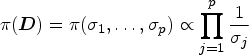
For model (2.1), we assume that the $τ_{j}$ -level quantile of the $j$ -th component in $y_{i}$ is a function of the $k$ -dimensional covariate $x_{i}$ which can be specified as $Q_{τ_{j}} (y_{i j} | x_{i}) = β_{τ_{j}}^{T} x_{i}$ for $j = 1, \dots, p$ , where the $β_{τ_{j}}$ is the $τ_{j}$ -th quantile coefficients vector corresponding to the $j$ -th response. Denoting $β_{τ} = (β_{τ_{1}}, \dots, β_{τ_{p}})^{T}$ is a $p \times k$ matrix of parameters with $β_{τ_{j}} = (β_{j 1}, \dots, β_{j k})^{T}$ . Based on the common method for univariate QR model, one can estimate each $β_{τ_{j}}$ marginally by minimizing the objective function $\sum_{i = 1}^{N} ρ_{τ_{j}} (y_{i j} - β_{τ_{j}}^{T} x_{i})$ , where $ρ_{τ_{j}} (\cdot)$ denotes the $τ_{j}$ -level univariate quantile check function. It can be noticed, however, that the estimators from the above objective functions totally ignore the dependence among the components in multivariate response $y_{i}$ . An alterative is to study the joint estimation of the $p$ conditional quantiles by incorporating the correlations into the components of the multivariate response $y_{i}$ . And for that, a MAL (multivariate asymmetric Laplace) distribution can be imposed on the error term $e_{i}$ of model (2.1) to specify the joint quantiles of $y_{i}$ conditionally on convarate $x_{i}$ . The pdf (probability density function) of the $p$ -variate random vector $Y$ for the three-parameter MAL distribution ${MAL}_{p} (α, ξ, Ω)$ is given as

g_{Y} (y | α, ξ, Ω) = \frac{2 exp [(y - α)^{T} Ω^{- 1} ξ]}{(2 π)^{p / 2} | Ω |^{1 / 2}} (\frac{κ}{2 + d})^{υ / 2} \cdot K_{υ} (\sqrt{(2 + d) κ})

where

d = ξ^{T} Ω^{- 1} ξ

κ = (y - α)^{T} Ω^{- 1} (y - α)

α

and

ξ

are the shift and shape parameters, respectively,

Ω

is the

p \times p

positive definite matrix of scale parameters, and

K (\cdot)

denotes the modified Bessel function of the third kind with index parameter

ν = (2 - p) / 2

. One can refer to Kotz et al.,⁴⁰ Kollo and Srivastava,⁴¹ Visk,⁴² and Hurlimann⁴³ for more disscussion on the MAL distribution. Letting

D = diag (σ_{1}, \dots, σ_{p})

with

σ_{j} > 0

ξ = D θ

and

Ω = D Σ D

, one can reparameterize the distribution

{MAL}_{p} (0, D θ, D Σ D)

for

e_{i}

or the conditional distribution

{MAL}_{p} (β_{τ} x_{i}, D θ, D Σ D)

for

y_{i}

in model (2.1), where

θ = (θ_{1}, \dots, θ_{p})^{T}

has generic element

θ_{j} = \frac{1 - 2 τ_{j}}{(τ_{j} (1 - τ_{j})}

Σ

is a

p \times p

positive matrix such that

Σ = \nabla Ψ \nabla

, and

Ψ

being a correlation matrix and

\nabla = diag (δ_{1}, \dots, δ_{p})

with

δ_{j}^{2} = \frac{1}{τ_{j} (1 - τ_{j})}

. The unknown parameters include

β_{τ}

Ψ

, and

D

(i.e.

σ = (σ_{1}, \dots, σ_{p})

Petrella and Raponi³⁸ showed that the $j$ -th marginal distribution of $y_{i}$ under the assumption of MAL distribution is an univariate asymmetric Laplace distribution $AL (β_{τ_{j}}^{T} x_{i}, τ_{j}, σ_{j})$ . Besides, the correlations among the components of multivariate response $y_{i}$ are included in the matrix $Σ$ (or $Ψ$ ). It is noticed that the density of MAL distribution is too complex for conducting statistical inference. To make statistical inference simpler, a hierarchical representation of the response $y_{i}$ can be given as follows:

y_{i} = β_{τ} x_{i} + D θ w_{i} + \sqrt{w_{i}} D Σ^{1 / 2} z_{i}

(2.2)

where

z_{i}

follow the

p

-variate standard normal distribution

N_{p} (0, I_{p})

w_{i}

are latent variables which follow the standard exponential distribution

Exp (1)

, and

z_{i}

are independent of

w_{i}

. Conditioning on

w_{i}

y_{i}

follow the multivariate normal distribution with the mean

β_{τ} x_{i} + D θ w_{i}

and variance–covariane matrix

w_{i} D Σ D

. In the following sections, we will investigate Bayesian joint QR approach for the multivariate longitudinal mixed effect model and its application.

3. Model specification

3.1. The multi-response longitudinal mixed-effect model

Suppose a data set comes from a unbalanced longitudinal study with $N$ subjects and each subject has $n_{i}$ repeated measurements over time. Each measurement has $p$ characteristic responses for each subject. Let $y_{i t} = (y_{i t}^{(1)}, \dots, y_{i t}^{(p)})^{T}$ be the observation vector of the $p$ responses for the $i$ -th individual measured at the $t$ -th time ( $i = 1, \dots, N; t = 1, \dots, n_{i}$ ). The multi-response mixed-effects models with a random intercept can be expressed as follows:

y_{i t}^{(j)} = x_{i t}^{T} β_{j} + b_{i}^{(j)} + e_{i t}^{(j)}, j = 1, \dots, p

(3.1)

where

y_{i t}^{(j)}

is the

t

-th observation of the

i

-th individual for

j

-th variate response,

x_{i t}

is a

k \times 1

vector of covariates,

β_{j}

is a

k \times 1

unknown parameter vector of fixed effects for the

j

-th response,

b_{i}^{(j)}

is the

j

-th random intercept term specific to subject

i

e_{i t}^{(j)}

is the error term.

The vector expression of model (3.1) is

y_{i t} = β x_{i t} + b_{i} + e_{i t}

(3.2)

where

e_{i t} = (e_{i t}^{(1)}, \dots, e_{i t}^{(p)})^{T}

β = (β_{1}, \dots, β_{p})^{T}

, and

b_{i} = (b_{i}^{(1)}, \dots, b_{i}^{(p)})^{T}

. The random effect

b_{i}

is simply supposed to follow

p

-variate normal distribution

N_{p} (0, Σ_{b})

for each subject, in which

Σ_{b}

is a

p \times p

variance–covariance matrix. Random effects

b_{i}

in model (3.2) accounts for the longitudinal association of data from the same individual across time. The diagonal elements of

Σ_{b}

quantify the variability between subjects, and the off-diagonal elements of

Σ_{b}

measure the overall association between responses.

In the framework of QR modeling, we specify the $τ_{j}$ -th marginal quantile of response $y_{i t}^{(j)}$ conditionally on $x_{i t}$ and $b_{i}^{(j)}$ in model (3.1) as follows:

Q_{τ_{j}} (y_{i t}^{(j)} | x_{i t}, b_{i}) = x_{i t}^{T} β_{τ_{j}} + b_{i}^{(j)}

(3.3)

Model (3.3) considers the marginal quantile of response

y_{i t}^{(j)}

and totally ignores the dependences among the components of

y_{i t}

. In order to implement the joint QR analysis, based on the preliminaries in Section 2, a multivariate distribution

{MAL}_{p} (0, D θ, D Σ D)

is specified on the error term

e_{i t}

of model (3.2). Similarly to model (2.5), go a step further, we obtain the hierarchical representation of model (3.2) conditionally on the random effects

b_{i}

as follows:

y_{i t} = β_{τ} x_{i t} + b_{i} + D θ w_{i t} + \sqrt{w_{i t}} {D Σ}^{1 / 2} z_{i t}, i = 1, \dots, N, t = 1, \dots, n_{i}

(3.4)

where

β_{τ} = (β_{τ_{1}}, \dots, β_{τ_{p}})^{T}

z_{i t}

follow the

p

-variate standard normal distribution

N_{p} (0, I_{p})

w_{i t}

follow the standard exponential distribution

Exp (1)

and are independent of

z_{i t}

. For model (3.4), conditioning on latent variable

w_{i t}

and random effect

b_{i}

y_{i t}

follows the multivariate normal distribution with the mean

β_{τ} x_{i t} + b_{i} + D θ w_{i t}

and variance–covariane matrix

w_{i t} D Σ D

, namely

y_{i t} | x_{i t}, b_{i}, w_{i t} \sim N (β_{τ} x_{i t} + b_{i} + D θ w_{i t}, w_{i t} D Σ D)

(3.5)

3.2. The complete joint hierarchical likelihood

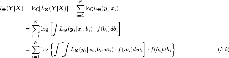
Denote $Θ = {β_{τ}, Ψ, D, Σ_{b}}$ , $Y = {y_{1}, \dots, y_{N}}$ , $X = {x_{1}, \dots, x_{N}}$ , and $W = {w_{1}, \dots, w_{N}}$ . In model (3.4), the random effect $b_{i}$ and $w_{i t}$ are unobserved latent variables. Hence, the observed log-likelihood function is

\begin{aligned} l_{Θ} (Y | X) & = log [L_{Θ} (Y | X)] = \sum_{i = 1}^{N} log L_{Θ} (y_{i} | x_{i}) \\ = \sum_{i = 1}^{N} log [\int L_{Θ} (y_{i} | x_{i}, b_{i}) \cdot f (b_{i}) d b_{i}] \\ = \sum_{i = 1}^{N} log {\int [\int L_{Θ} (y_{i} | x_{i}, b_{i}, w_{i}) \cdot f (w_{i}) d w_{i}] \cdot f (b_{i}) d b_{i}} \end{aligned}

(3.6)

where

y_{i} = {y_{i 1}, \dots, y_{i n_{i}}}

x_{i} = {x_{i 1}, \dots, x_{i n_{i}}}

w_{i} = {w_{i 1}, \dots, w_{i n_{i}}}

L_{Θ} (y_{i} | x_{i}, b_{i}, w_{i})

is the pdf of

y_{i}

conditionally on

b_{i}

and

w_{i}

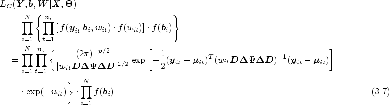
It is difficult to maximize the above marginal log-likelihood (3.6). We address this problem using the MCMC algorithm in Bayesian framework. We firstly present the joint hierarchical working likelihood of the complete data ${Y, b, W}$ for model (3.4) as follows:

\begin{aligned} L_{C} (Y, b, W | X, Θ) \\ = \prod_{i = 1}^{N} {\prod_{t = 1}^{n_{i}} [f (y_{i t} | b_{i}, w_{i t}) \cdot f (w_{i t})] \cdot f (b_{i})} \\ = \prod_{i = 1}^{N} \prod_{t = 1}^{n_{i}} {\frac{(2 π)^{- p / 2}}{| w_{i t} D Δ Ψ Δ D |^{1 / 2}} \exp [- \frac{1}{2} (y_{i t} - μ_{i t})^{T} (w_{i t} D Δ Ψ Δ D)^{- 1} (y_{i t} - μ_{i t})] \\ \cdot \exp (- w_{i t})} \cdot \prod_{i = 1}^{N} f (b_{i}) \end{aligned}

(3.7)

where

μ_{i t} = β_{τ} x_{i t} + b_{i} + D θ w_{i t}

4. Bayesian estimation approach

4.1. Prior specifications

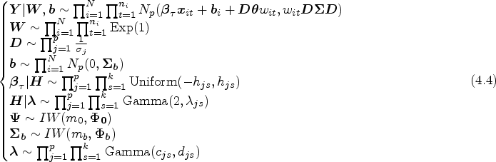
To select important covariates for improving prediction accuracy, various regularized penalization methods are used to conduct variable selection. Commonly used penalty functions mainly include LASSO (least absolute shrinkage and selection operator) penalty, ridge penalty, SCAD (smoothly clipped absolute deviation) penalty as well as bridge penalty. More discussion on LASSO penalty and Bayesian LASSO can be found by Tibshirani,⁴⁴ Zou,⁴⁵ Park and Casella,⁴⁶ Leng,⁴⁷ etc. This article considers Bayesian adaptive LASSO regularization of regression parameters in model (3.2). In order to do this, we impose the Laplace priors for regression parameters $β_{τ}$ as follows:

π (β_{τ}) = \prod_{j = 1}^{p} π (β_{τ_{j}}), π (β_{τ_{j}}) = \prod_{s = 1}^{k} π (β_{j s} | λ_{j s}), π (β_{j s} | λ_{j s}) = \frac{λ_{j s}}{2} \exp {- λ_{j s} | β_{j s} |}

(4.1)

where

λ = {λ_{j s}}, λ_{j s} > 0

are tuning parameters.

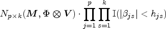
However, the prior in (4.1) is analytically intractable to calculate the desirable posterior quantities. Using the mixture representation approach by Mallick and Yi (2018), we decompose the prior of $β_{j, s}$ as the following uniform–gamma mixture representation,

π (β_{j s} | λ_{j s}) = \int_{0}^{\infty} π (β_{j s} | h_{j s}) \cdot π (h_{j s} | λ_{j s}) d h_{j s}

where

π (β_{j s} | h_{j s}) = Uniform (- h_{j s}, h_{j s}), π (h_{j s} | λ_{j s}) = Gamma (2, λ_{j s}) .

The joint prior of $β_{τ}$ can be represented as

π (β_{τ} | H, λ) \propto \prod_{j = 1}^{p} \prod_{s = 1}^{k} [π (β_{j s} | h_{j s}) \cdot π (h_{j s} | λ_{j s})]

where

H = {h_{j s}}

The prior of $Σ_{b}$ is set as inverse Wishart distribution: $π (Σ_{b}) \sim IW (m_{b}, Φ_{b})$ .

The prior of $Ψ$ is set as inverse Wishart distribution: $π (Ψ) \sim IW (m_{0}, Φ_{0})$ .

The prior of $D$ is assumed to be the following informative prior

π (D) = π (σ_{1}, \dots, σ_{p}) \propto \prod_{j = 1}^{p} \frac{1}{σ_{j}}

The prior of

λ

is set as

π (λ) = \prod_{j = 1}^{p} \prod_{s = 1}^{k} π (λ_{j s})

, where

λ_{j s} \sim Gamma (c_{j s}, d_{j s}) .

Hence, the joint hierarchical prior of all parameters is

π (Θ, λ) \propto π (β_{τ} | H, λ) π (Σ_{b}) π (Ψ) π (D) π (λ)

(4.2)

4.2. The fully conditional posteriors and Gibbs sampling algorithm

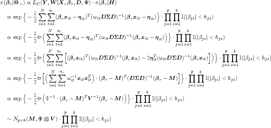
Incorporating joint prior (4.2) into the joint working likelihood (3.7) results in the joint posterior density of all parameters as follows:

π (Θ, λ, b, W, Y | X) \propto L_{C} (Y, b, W | X, Θ) \cdot π (Θ, λ)

(4.3)

Gibbs sampler procedures are employed to carry MCMC algorithm. The hierarchical expression of posterior distributions of all unknown parameters and latent variables can be presented as follows:

{\begin{cases} Y | W, b \sim \prod_{i = 1}^{N} \prod_{t = 1}^{n_{i}} N_{p} (β_{τ} x_{i t} + b_{i} + D θ w_{i t}, w_{i t} D Σ D) \\ W \sim \prod_{i = 1}^{N} \prod_{t = 1}^{n_{i}} Exp (1) \\ D \sim \prod_{j = 1}^{p} \frac{1}{σ_{j}} \\ b \sim \prod_{i = 1}^{N} N_{p} (0, Σ_{b}) \\ β_{τ} | H \sim \prod_{j = 1}^{p} \prod_{s = 1}^{k} Uniform (- h_{j s}, h_{j s}) \\ H | λ \sim \prod_{j = 1}^{p} \prod_{s = 1}^{k} Gamma (2, λ_{j s}) \\ Ψ \sim I W (m_{0}, Φ_{0}) \\ Σ_{b} \sim I W (m_{b}, Φ_{b}) \\ λ \sim \prod_{j = 1}^{p} \prod_{s = 1}^{k} Gamma (c_{j s}, d_{j s}) \end{cases}

(4.4)

Let

Θ_{-}

denote the remaining parameters subset apart from the present sample parameter. The full conditional posterior distributions of unknown parameters and latent variables can be presented as follows, respectively.

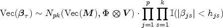
$∙$ Sample $β_{τ}$ from the truncated matrix normal distribution

N_{p \times k} (M, Φ \otimes V) \cdot \prod_{j = 1}^{p} \prod_{s = 1}^{k} I (| β_{j s} | < h_{j s})

In terms of the properties of matrix normal distribution, we have

Vec (β_{τ}) \sim N_{p k} (Vec (M), Φ \otimes V) \cdot \prod_{j = 1}^{p} \prod_{s = 1}^{k} I (| β_{j s} | < h_{j s})

Specially, we can marginally sample the component

β_{j s}

Vec (β_{τ})

via the following truncated normal distribution:

N (Vec (M)_{(s - 1) p + j}, (Φ \otimes V)_{(s - 1) p + j, (s - 1) p + j}) \cdot I (| β_{j s} | < h_{j s}), j = 1, \dots, p, s = 1, \dots, k

The theoretical posterior distribution of

β_{τ}

is derived as follows:

\begin{aligned} π (β_{τ} | Θ_{-}) \propto L_{C} (Y, W | X, β_{τ}, D, Ψ) \cdot π (β_{τ} | H) \\ \propto \exp {- \frac{1}{2} \sum_{i = 1}^{N} \sum_{t = 1}^{n_{i}} (β_{τ} x_{i t} - η_{i t})^{T} (w_{i t} D Σ D)^{- 1} (β_{τ} x_{i t} - η_{i t})} \cdot \prod_{j = 1}^{p} \prod_{s = 1}^{k} I (| β_{j s} | < h_{j s}) \\ \propto \exp {- \frac{1}{2} t r (\sum_{i = 1}^{N} \sum_{t = 1}^{n_{i}} (β_{τ} x_{i t} - η_{i t})^{T} (w_{i t} D Σ D)^{- 1} (β_{τ} x_{i t} - η_{i t}))} \cdot \prod_{j = 1}^{p} \prod_{s = 1}^{k} I (| β_{j s} | < h_{j s}) \\ \propto \exp {- \frac{1}{2} t r (\sum_{i = 1}^{N} \sum_{t = 1}^{n_{i}} [(β_{τ} x_{i t})^{T} (w_{i t} D Σ D)^{- 1} (β_{τ} x_{i t}) - 2 η_{i t}^{T} (w_{i t} D Σ D)^{- 1} (β_{τ} x_{i t})])} \cdot \prod_{j = 1}^{p} \prod_{s = 1}^{k} I (| β_{j s} | < h_{j s}) \\ \propto \exp {- \frac{1}{2} t r [(\sum_{i = 1}^{N} \sum_{t = 1}^{n_{i}} w_{i t}^{- 1} x_{i t} x_{i t}^{T}) \cdot (β_{τ} - M)^{T} (D Σ D)^{- 1} (β_{τ} - M)]} \cdot \prod_{j = 1}^{p} \prod_{s = 1}^{k} I (| β_{j s} | < h_{j s}) \\ \propto \exp {- \frac{1}{2} t r (Φ^{- 1} \cdot (β_{τ} - M)^{T} V^{- 1} (β_{τ} - M))} \cdot \prod_{j = 1}^{p} \prod_{s = 1}^{k} I (| β_{j s} | < h_{j s}) \\ \sim N_{p \times k} (M, Φ \otimes V) \cdot \prod_{j = 1}^{p} \prod_{s = 1}^{k} I (| β_{j s} | < h_{j s}) \end{aligned}

where

N_{p \times k} (M, Φ \otimes V)

denotes a

p \times k

matrix normal distribution with parameters

M

Φ

V

, and

Φ = (\sum_{i = 1}^{N} \sum_{t = 1}^{n_{i}} w_{i t}^{- 1} x_{i t} x_{i t}^{T})^{- 1}

M = \sum_{i = 1}^{N} \sum_{t = 1}^{n_{i}} (w_{i t}^{- 1} η_{i t} x_{i t}^{T}) \cdot Φ

V = D Σ D

, and

η_{i t} = y_{i t} - b_{i} - D θ w_{i t}

$∙$ Sample $σ_{j}$ from the following posterior distribution:

\begin{aligned} π (σ_{j} | Θ_{-}) \\ \propto | D |^{- (\sum_{i = 1}^{N} n_{i} + 1)} \exp {- \frac{1}{2} t r [\sum_{i = 1}^{N} \sum_{t = 1}^{n_{i}} (e_{i t} - D θ w_{i t})^{T} (w_{i t} D Σ D)^{- 1} (e_{i t} - D θ w_{i t})]} \\ \propto σ_{j}^{- (\sum_{i = 1}^{N} n_{i} + 1)} \cdot \exp {- \frac{1}{2} t r [\sum_{i = 1}^{N} \sum_{t = 1}^{n_{i}} (w_{i t}^{- 1} e_{i t} e_{i t}^{T}) \cdot (D^{- 1} Σ^{- 1} D^{- 1}) - θ (\sum_{i = 1}^{N} \sum_{t = 1}^{n_{i}} e_{i t}^{T}) \cdot Σ^{- 1} D^{- 1}]} \end{aligned}

where

e_{i t} = y_{i t} - β_{τ} x_{i t} - b_{i}

Noting that $π (σ_{j} | Θ_{-})$ is not a standard distribution, we can sample $σ_{j}$ using the MH (Metropolis-Hastings) algorithm by the following steps: (I)

Generate a random number $σ_{j}^{c a n d i d a t e}$ from the truncated normal distribution $TN (0, γ^{2}, 0, \infty)$ which is specified as the proposal distribution in the MH algorithm, where $γ^{2}$ denotes the hyperparameter of variance and $(0, \infty)$ is the sampling interval of the truncated normal distribution. The pdf of the proposal distribution is denoted as $q (\cdot | Θ_{-})$ .

(II)

Generate a random number $u$ from the standard uniform distribution $U [0, 1]$ .

(III)

Compute the acceptance probability $r = min {1, \frac{q (σ_{j}^{o l d} | Θ_{-})}{q (σ_{j}^{c a n d i d a t e} | Θ_{-})} \cdot \frac{π (σ_{j}^{c a n d i d a t e} | Θ_{-})}{π (σ_{j}^{o l d} | Θ_{-})}}$

(IV)

If $u < r$ , then accept the proposal $σ_{j} \leftarrow σ_{j}^{c a n d i d a t e}$ , otherwise reject the proposal and let $σ_{j} \leftarrow σ_{j}^{o l d}$ .

•

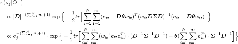
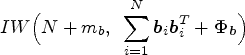
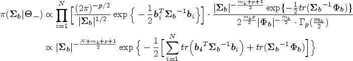
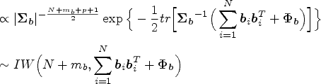
Sample $Ψ$ from the following inverse Wishart distribution:

I W (\sum_{i = 1}^{N} n_{i} + m_{0}, (\nabla D)^{- 1} \cdot \sum_{i = 1}^{N} \sum_{t = 1}^{n_{i}} (w_{i t}^{- 1} α_{i t} α_{i t}^{T}) \cdot (D \nabla)^{- 1} + Φ_{0})

The theoretical posterior distribution of

Ψ

is as follows:

\begin{aligned} π (Ψ | Θ_{-}) \propto L_{C} (Y, b, W | X, β_{τ}, D, Ψ, Σ_{b}) \cdot π (Ψ) \\ \propto \prod_{i = 1}^{N} \prod_{t = 1}^{n_{i}} [\frac{(2 π)^{- p / 2}}{| w_{i t} D \nabla Ψ \nabla D |^{1 / 2}} \exp {- \frac{1}{2} α_{i t}^{T} (w_{i t} D \nabla Ψ \nabla D)^{- 1} α_{i t}}] \frac{| Ψ |^{- \frac{m_{0} + p + 1}{2}} \exp {- \frac{1}{2} t r (Ψ^{- 1} Φ_{0})}}{2^{\frac{m_{0} p}{2}} | Φ_{0} |^{- \frac{m_{0}}{2}} \cdot Γ_{p} (\frac{m_{0}}{2})} \\ \propto | Ψ |^{- \frac{\prod_{i = 1}^{N} n_{i} + m_{0} + p + 1}{2}} \exp {- \frac{1}{2} [\sum_{i = 1}^{N} \sum_{t = 1}^{n_{i}} t r (α_{i t}^{T} (w_{i t} D \nabla Ψ \nabla D)^{- 1} α_{i t}) + t r (Ψ^{- 1} Φ_{0})]} \\ \propto | Ψ |^{- \frac{\prod_{i = 1}^{N} n_{i} + m_{0} + p + 1}{2}} \exp {- \frac{1}{2} t r [Ψ^{- 1} ((\nabla D)^{- 1} \cdot \sum_{i = 1}^{N} \sum_{t = 1}^{n_{i}} (w_{i t}^{- 1} α_{i t} α_{i t}^{T}) \cdot (D \nabla)^{- 1} + Φ_{0})]} \\ \sim I W (\prod_{i = 1}^{N} n_{i} + m_{0}, (\nabla D)^{- 1} \cdot \sum_{i = 1}^{N} \sum_{t = 1}^{n_{i}} (w_{i t}^{- 1} α_{i t} α_{i t}^{T}) \cdot (D \nabla)^{- 1} + Φ_{0}) \end{aligned}

where

α_{i t} = y_{i t} - β_{τ} x_{i t} - b_{i} - D θ w_{i t}

•

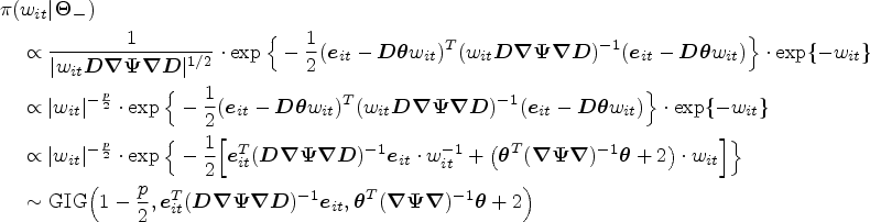
Sample $w_{i t}$ from the generalized inverse Gaussian distribution

GIG (1 - \frac{p}{2}, e_{i t}^{T} (D Σ D)^{- 1} e_{i t}, θ^{T} Σ^{- 1} θ + 2)

The theoretical posterior distribution of

w_{i t}

is derived as follows:

\begin{aligned} π (w_{i t} | Θ_{-}) \\ \propto \frac{1}{| w_{i t} D \nabla Ψ \nabla D |^{1 / 2}} \cdot \exp {- \frac{1}{2} (e_{i t} - D θ w_{i t})^{T} (w_{i t} D \nabla Ψ \nabla D)^{- 1} (e_{i t} - D θ w_{i t})} \cdot \exp {- w_{i t}} \\ \propto | w_{i t} |^{- \frac{p}{2}} \cdot \exp {- \frac{1}{2} (e_{i t} - D θ w_{i t})^{T} (w_{i t} D \nabla Ψ \nabla D)^{- 1} (e_{i t} - D θ w_{i t})} \cdot \exp {- w_{i t}} \\ \propto | w_{i t} |^{- \frac{p}{2}} \cdot \exp {- \frac{1}{2} [e_{i t}^{T} (D \nabla Ψ \nabla D)^{- 1} e_{i t} \cdot w_{i t}^{- 1} + (θ^{T} (\nabla Ψ \nabla)^{- 1} θ + 2) \cdot w_{i t}]} \\ \sim GIG (1 - \frac{p}{2}, e_{i t}^{T} (D \nabla Ψ \nabla D)^{- 1} e_{i t}, θ^{T} (\nabla Ψ \nabla)^{- 1} θ + 2) \end{aligned}

•

Sample $λ_{j s}$ from the Gamma distribution: $Gamma (2 + c_{j s}, d_{j s} + h_{j s}) .$

•

Sample $h_{j s}$ from the left-truncated exponential distribution $Exp (λ_{j s}) I {h_{j s} > | β_{j s} |}$ , using the inversion method, which can be conducted by the following two steps: (I)

Generate $h_{j s}^{*} \sim Exp (λ_{j s}) .$

(II)

Generate $h_{j s} = h_{j s}^{*} + | β_{j s} | .$

∙

Sample

Σ_{b}

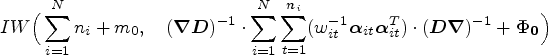
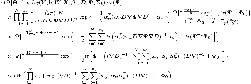
from the following inverse Wishart distribution

I W (N + m_{b}, \sum_{i = 1}^{N} b_{i} b_{i}^{T} + Φ_{b})

The theoretical derivation of the posterior distribution of

Σ_{b}

is as follows:

\begin{aligned} π (Σ_{b} | Θ_{-}) & \propto \prod_{i = 1}^{N} [\frac{(2 π)^{- p / 2}}{| Σ_{b} |^{1 / 2}} \exp {- \frac{1}{2} b_{i}^{T} Σ_{b}^{- 1} b_{i}}] \cdot \frac{| Σ_{b} |^{- \frac{m_{b} + p + 1}{2}} \exp {- \frac{1}{2} t r (Σ_{b}^{- 1} Φ_{b})}}{2^{\frac{m_{b} p}{2}} | Φ_{b} |^{- \frac{m_{b}}{2}} \cdot Γ_{p} (\frac{m_{b}}{2})} \\ \propto | Σ_{b} |^{- \frac{N + m_{b} + p + 1}{2}} \exp {- \frac{1}{2} [\sum_{i = 1}^{N} t r (b_{i}^{T} Σ_{b}^{- 1} b_{i}) + t r (Σ_{b}^{- 1} Φ_{b})]} \\ \propto | Σ_{b} |^{- \frac{N + m_{b} + p + 1}{2}} \exp {- \frac{1}{2} t r [Σ_{b}^{- 1} (\sum_{i = 1}^{N} b_{i} b_{i}^{T} + Φ_{b})]} \\ \sim I W (N + m_{b}, \sum_{i = 1}^{N} b_{i} b_{i}^{T} + Φ_{b}) \end{aligned}

•

Sample $b_{i}$ from normal distribution $N (μ_{b_{i}}^{*}, Σ_{b_{i}}^{*})$ , where $ς_{i t} = y_{i t} - β_{τ} x_{i t} - D θ w_{i j}$ , and $μ_{b_{i}}^{*} = Σ_{b_{i}}^{*} \cdot (D Σ D)^{- 1} \sum_{j = 1}^{n_{i}} w_{i t}^{- 1} ς_{i t}$ , $Σ_{b_{i}}^{*} = ((D Σ D)^{- 1} \sum_{j = 1}^{n_{i}} w_{i t}^{- 1} + Σ_{b}^{- 1})^{- 1}$ .

For carrying out a Bayesian analysis, an efficient MCMC algorithm is used to sample

β_{τ}, Ψ, W, H, b, Σ_{b}

, and

λ

from the above conditional posterior distributions. In particular, for correlation matrix

Ψ

, we draw its sample from the posterior inverse Wishart distribution, and then standardize it as the correlation coefficient matrix.

5. Simulation studies

In this section, we investigate the performance of the proposed Bayesian procedures by conducting some Monte Carlo simulations. We repeatedly generate 50 data sets from the following three-variate longitudinal mixed model

y_{i t} = β x_{i t} + b_{i} + e_{i t}, i = 1, \dots, N, t = 1, \dots, m

(5.1)

where

N = 20

and equal cluster sizes

m = 5

are considered to illustrate the finite-sample performance. In model (5.1), the elements of

x_{i t}

are independently generated from the standard normal distribution, random effects

b_{i}

is drawn from three-variate normal distribution with zero mean and covariance matrix

Σ_{b}

of dimension

3 \times 3

Σ_{b}

is constructed by simulating from a Wishart distribution with four degrees of freedom and a diagonal scale matrix with element 0.1.

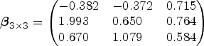
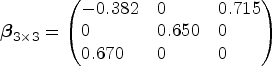
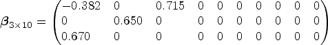
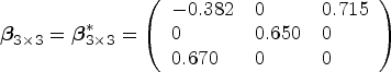
In model (5.1), the true parameter matrix $β$ is set as the following cases:

Model 1: Dense case:

\begin{aligned} β_{3 \times 3} = (\begin{array}{lll} - 0.382 & - 0.372 & 0.715 \\ 1.993 & 0.650 & 0.764 \\ 0.670 & 1.079 & 0.584 \end{array}) \end{aligned}

Model 2: Sparse case:

\begin{aligned} β_{3 \times 3} = (\begin{array}{lll} - 0.382 & 0 & 0.715 \\ 0 & 0.650 & 0 \\ 0.670 & 0 & 0 \end{array}) \end{aligned}

Model 3: Extremely sparse case:

\begin{aligned} β_{3 \times 10} = (\begin{array}{llllllllll} - 0.382 & 0 & 0.715 & 0 & 0 & 0 & 0 & 0 & 0 & 0 \\ 0 & 0.650 & 0 & 0 & 0 & 0 & 0 & 0 & 0 & 0 \\ 0.670 & 0 & 0 & 0 & 0 & 0 & 0 & 0 & 0 & 0 \end{array}) \end{aligned}

We set elements of matrices

D

and

Ψ

σ_{1} = 0.13, σ_{2} = 0.30, σ_{3} = 0.23

, and

ρ_{12} = 0.5, ρ_{13} = 0.3, ρ_{23} = 0.4

. Three cases of quantile levels, that is,

τ = (0.5, 0.5, 0.5)

τ = (0.25, 0.5, 0.75)

, and

τ = (0.75, 0.5, 0.25)

, are considered for the three models. Two different distributions for the error term

e_{i t}

in model (5.1) are considered as follows. Case I: A multivariate normal distribution (MN) with zero mean and a variance–covariance matrix equal to

{D θ θ}^{T} D + D Σ D

; Case II: A multivariate student t distribution with three degrees of freedom (Mt₃), non-centrality parameter

D θ

and scale parameter equal to

D Σ D

. An illustration of convergence diagnosis of the MCMC algorithm is shown in Section 5.1. The substantive calculations of the considered three models are implemented in Section 5.2. Section 5.3 provides some additional simulations.

Simulation studies in Section 5 and real-world data analysis in Section 6 are conducted on a Dell desktop [OptiPlex 7050, Intel(R) Core(TM) i7-7700U CPU] via statistical software R3.5.2. All codes of simulations and computations in this article can be requested on the first author. In addition, about the computation time, we conduct a test by taking the setting of $e_{i t} \sim {Mt}_{3}$ , $N = 20, m = 5$ , and $τ = (0.25, 0.5, 0.75)$ as an example. The computing times of the proposed joint QR approach for accomplishing one replication are 2.85 min for Model 1, 2.84 min for Model 2, and 2.89 min for Model 3, respectively.

5.1. Convergence diagnosis

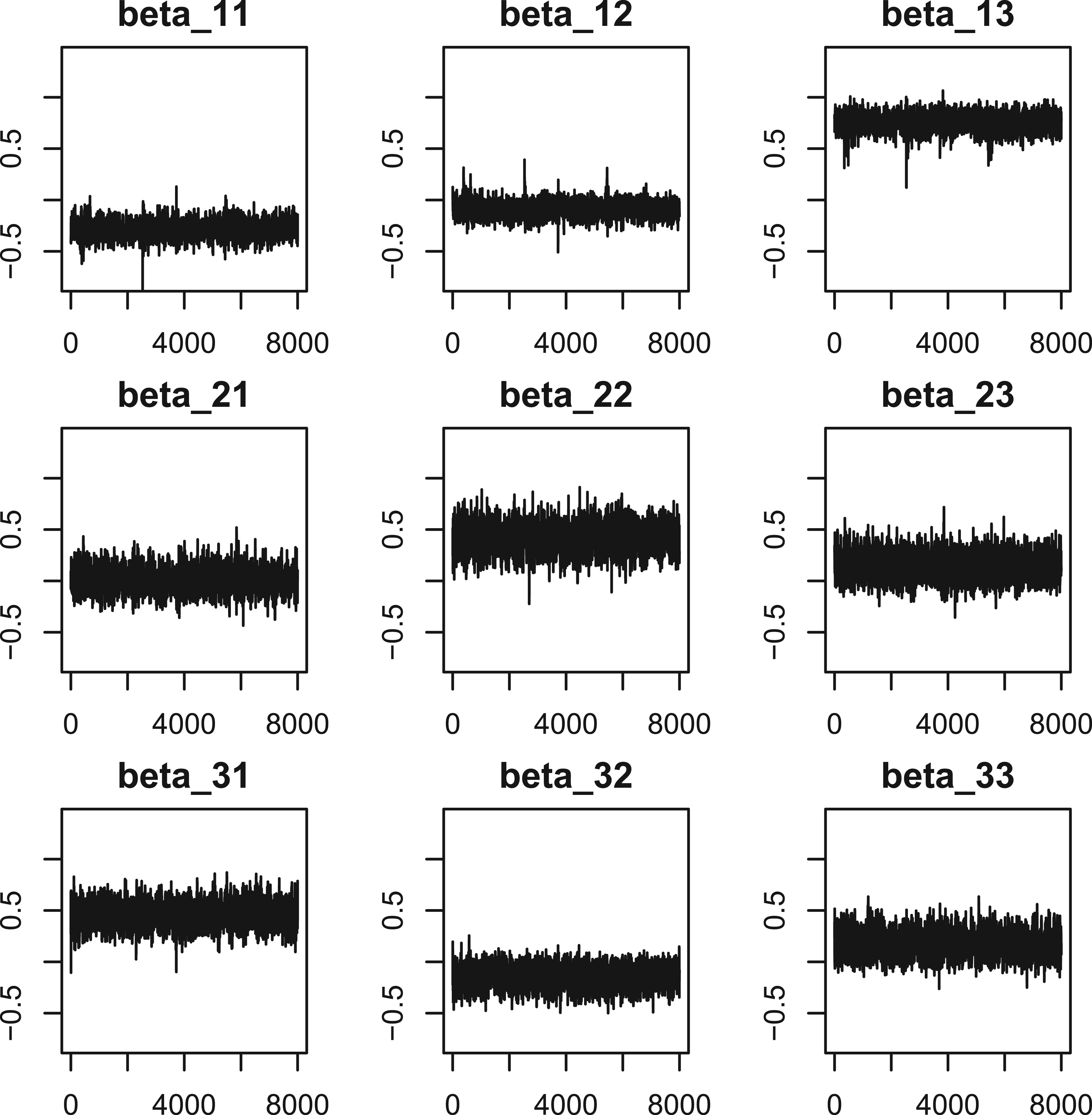
To guide the MCMC convergence, we carry out a few test runs under different initial values using the joint QR approach based on the settings of Model 2, and $e_{i t} \sim {Mt}_{3}$ (Case II) and $τ = (0.25, 0.5, 0.75)$ . The hyperparameters of the priors discussed in Section 4 are set as follows: $c = d = 0.1, m_{b} = 6, m_{0} = 4$ , $Φ_{0} = diag (1, \dots, 1), and Φ_{b} = diag (0.1, \dots, 0.1)$ . We consider three groups of initial values for parameters $β$ , $σ_{j}, j = 1, 2, 3$ and $Ψ$ as follows:

\begin{aligned} Initial values 1: β_{3 \times 3}^{(0)} & = (\begin{array}{lll} 1 & 1 & 1 \\ 1 & 1 & 1 \\ 1 & 1 & 1 \end{array}), Ψ^{(0)} = (\begin{array}{lll} 1 & 0 & 0 \\ 0 & 1 & 0 \\ 0 & 0 & 1 \end{array}), σ_{j}^{(0)} = 0.5, j = 1, 2, 3; \end{aligned}

\begin{aligned} Initialvalues 2: β_{3 \times 3}^{(0)} & = (\begin{array}{lll} 2 & 2 & 2 \\ 2 & 2 & 2 \\ 2 & 2 & 2 \end{array}), Ψ^{(0)} = (\begin{array}{lll} 1 & 0.3 & 0.3 \\ 0.3 & 1 & 0.3 \\ 0.3 & 0.3 & 1 \end{array}), σ_{j}^{(0)} = 5, j = 1, 2, 3; \end{aligned}

\begin{aligned} Initial values 3: β_{3 \times 3}^{(0)} & = (\begin{array}{lll} - 2 & - 2 & - 2 \\ - 2 & - 2 & - 2 \\ - 2 & - 2 & - 2 \end{array}), Ψ^{(0)} = (\begin{array}{lll} 1 & 0.8 & 0.8 \\ 0.8 & 1 & 0.8 \\ 0.8 & 0.8 & 1 \end{array}), σ_{j}^{(0)} = 10, j = 1, 2, 3. \end{aligned}

Initial values of other parameters were simply set as

b_{i}^{(0)} \sim N_{p} (0, I_{p})

Σ_{b}^{(0)} = I_{p}

Ψ^{(0)} = I_{p}

λ_{j s}^{(0)} \sim E x p (1)

h_{j s}^{(0)} \sim E x p (1)

, and

w_{i t}^{(0)} \sim E x p (1)

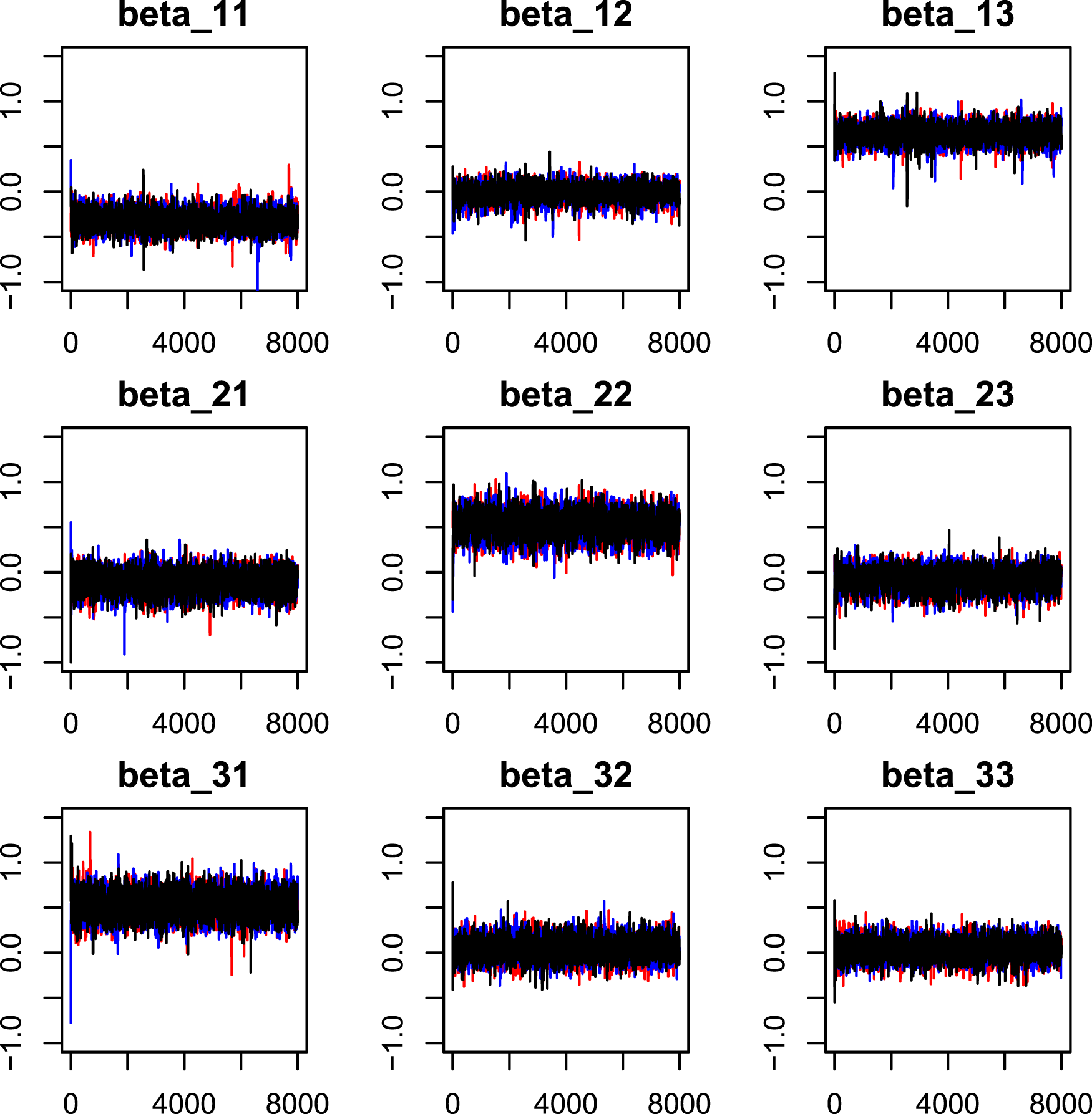
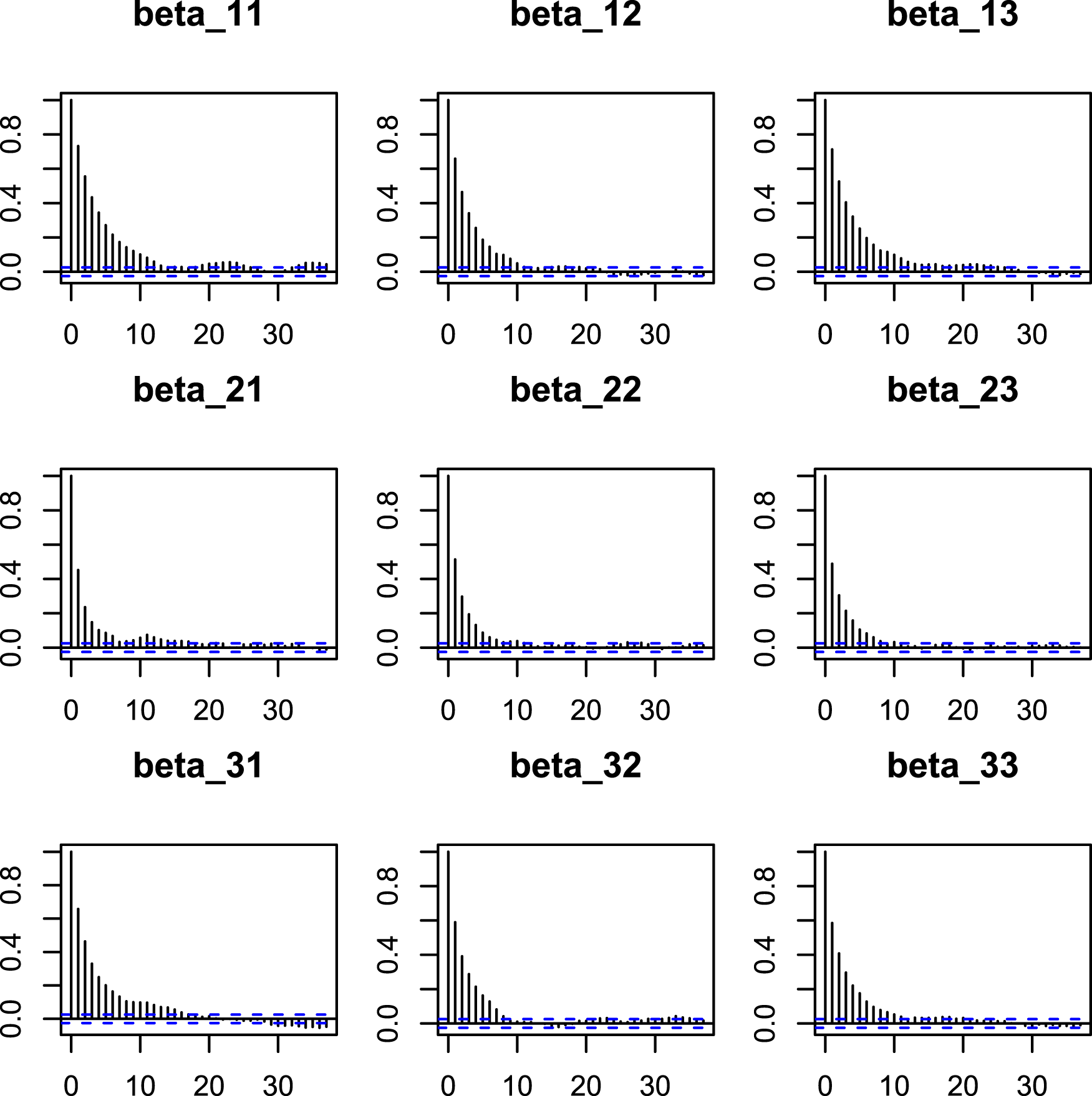
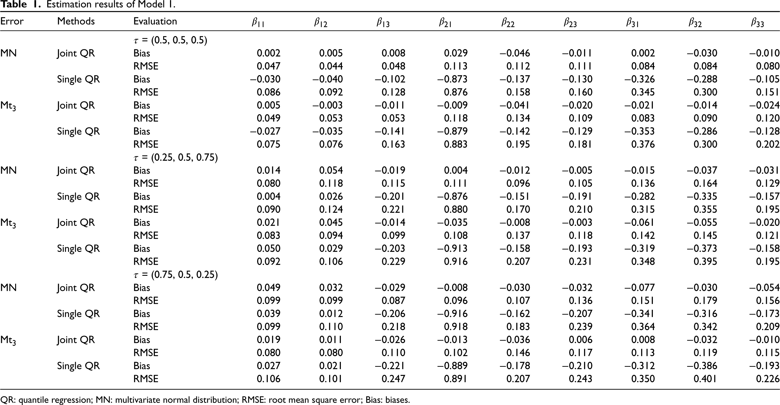
To be conservative, for each simulation, we run the Gibbs sampling algorithm 8000 iterations to assess the convergence of the MCMC algorithm. The MCMC trace plots under three initial values are displayed in Figures 1 and 2. It can be seen in Figure 1, three MCMC chains of regression coefficients starting from the above three initial values are mixed rapidly which shows a sufficient convergence of the algorithm. Figure 2 presents the trace plots of all 8000 posterior iterations of one MCMC chain for all regression coefficients under the setting of Initial values 1, which reconfirm that the MCMC chains rapidly converge to their stationary distributions. We also depict the autocorrelation function (ACF) plots in Figure 3 by discarding the first 2000 burn-in iterations to check the autocorrelation between stationary posterior samples under the setting of Initial values 1.

Figure 1.

MCMC chains starting from different initial values of the proposed joint QR. Note: The red line denotes the first setting of initial values; the blue line denotes the second setting; and the black line denotes the third setting. MCMC: Markov chain Monte Carlo; QR: quantile regression.

Figure 2.

Markov chain Monte Carlo (MCMC) trace plots.

Figure 3.

Autocorrelation function (ACF) plots.

5.2. Substantive simulations

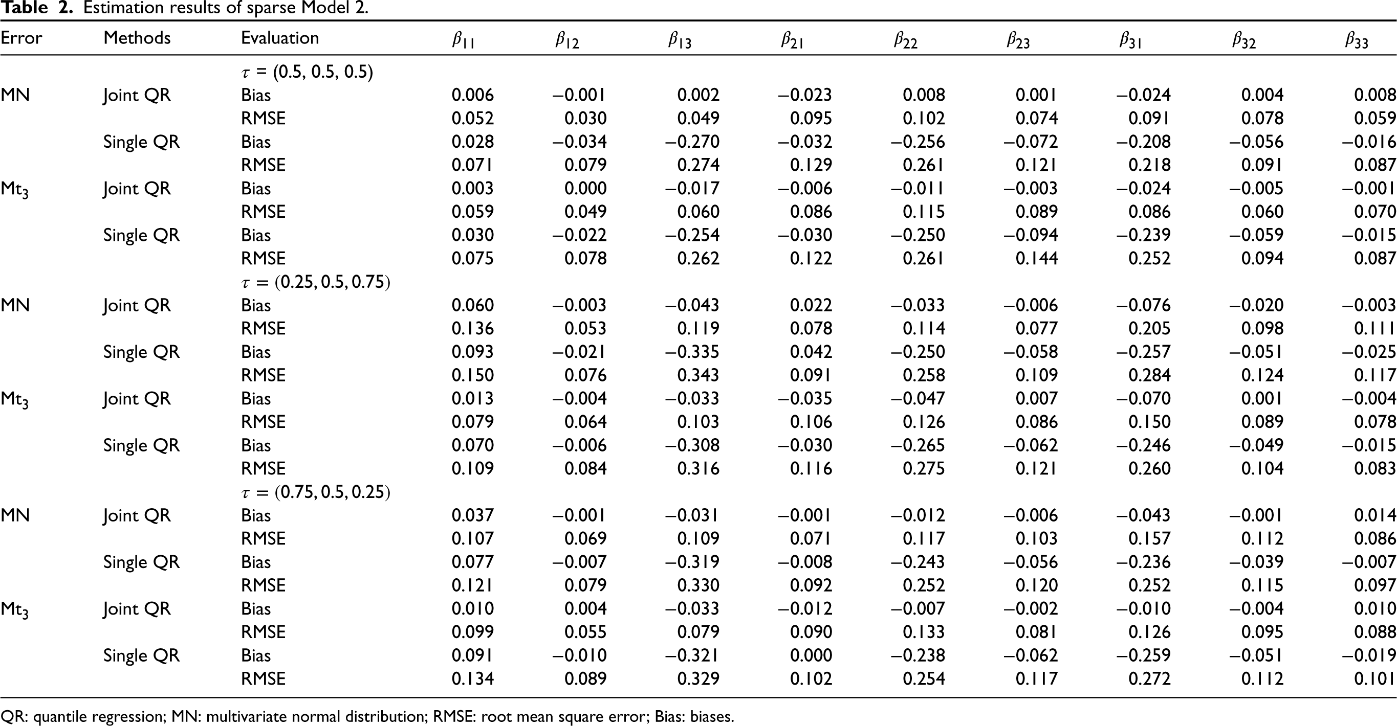
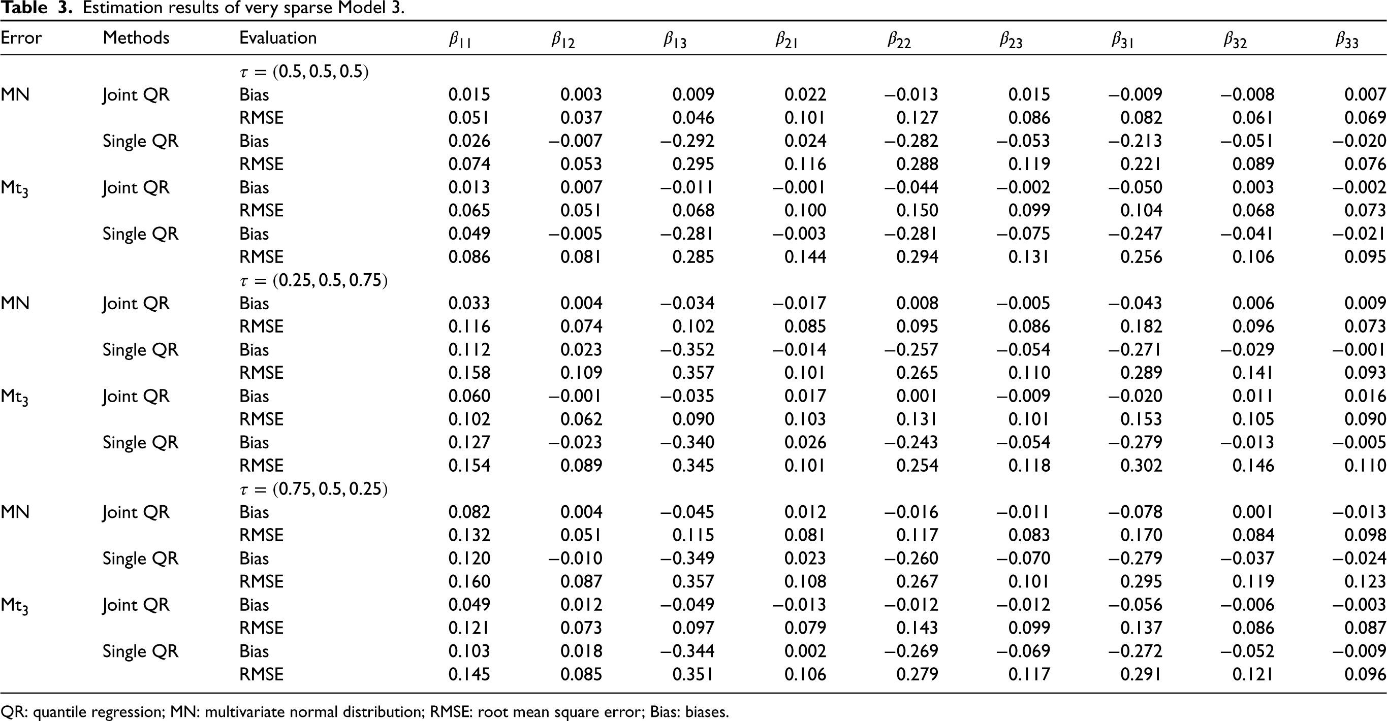
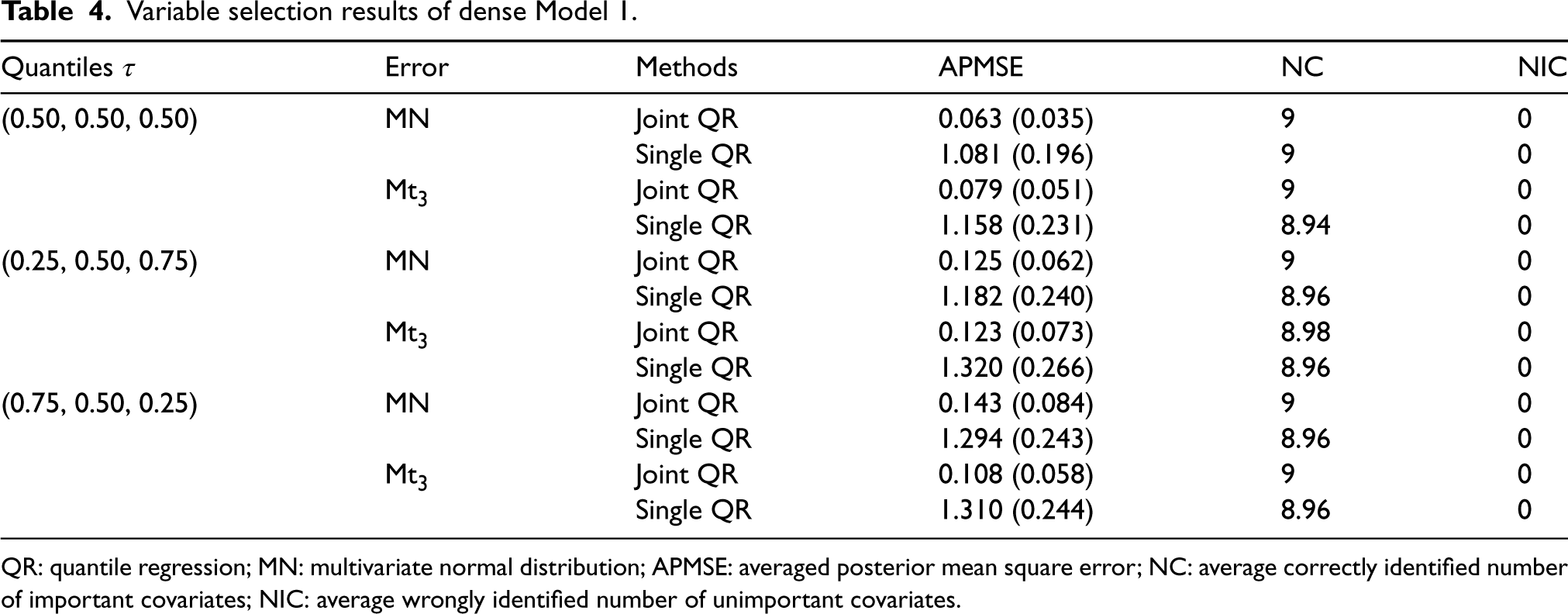
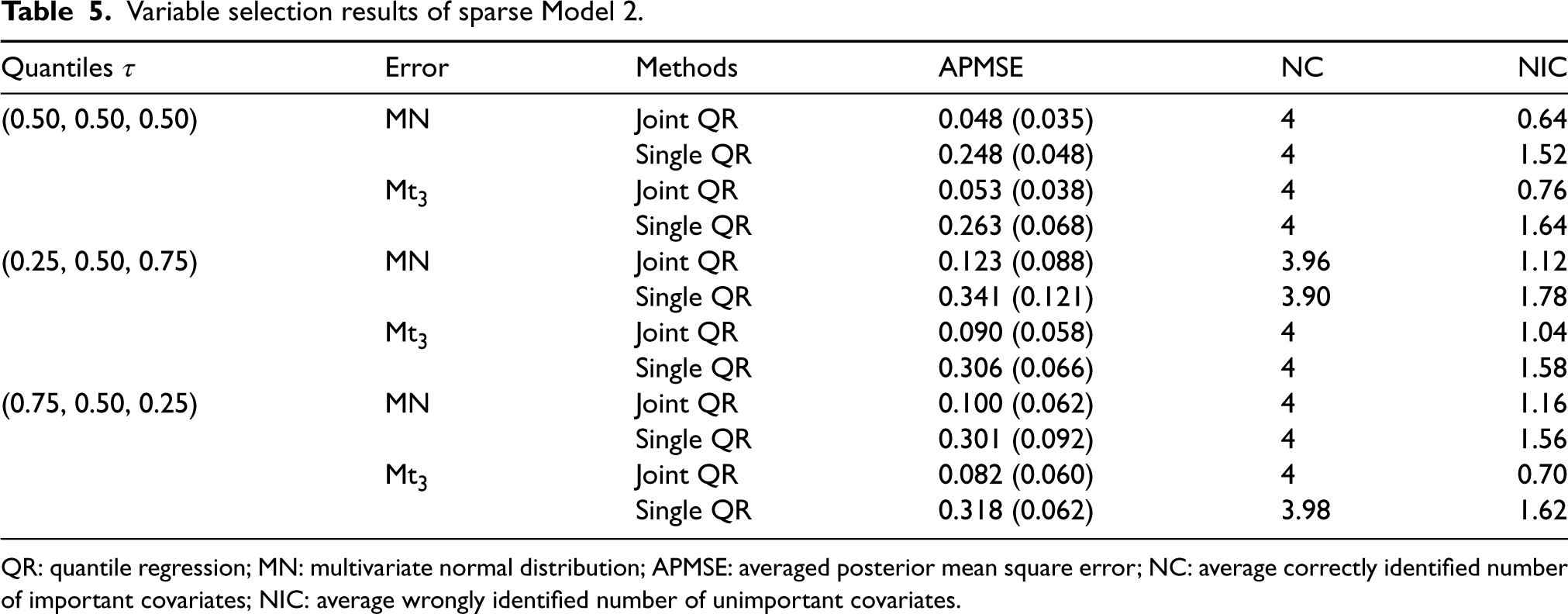
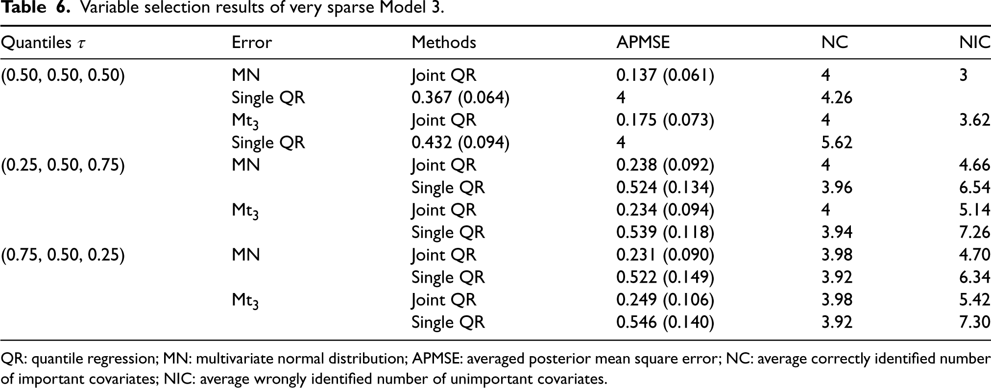
Parameters estimation and variable selection using the proposed Bayesian joint QR approach are conducted for dense Model 1 and sparse Models 2 and 3. The initial values of all parameters are set as the case of Initial values 1. The hyperparameters of priors are taken as the same values in Section 5.1. To illustrate the superiority of the joint QR approach, we also provide the estimation results of the single QR approach for each response for the aim of comparison. Fifty repeated simulations are conducted by running the Gibbs sampling algorithm for each model and each quantile combination. For each case, we run $8000$ iterations of Gibbs sampling algorithm for all parameters and latent variables, the first 2000 burn-in iterations are discarded and the remaining 6000 stationary iterations are retained to conduct posterior inference. Based on $50$ repeated simulations, the averaged estimation biases (Bias) and root mean square error (RMSE) of regression parameters for different settings are reported in Tables 1 to 3. A total of $95 %$ credible intervals for the regression coefficients are omitted here. For sparse models, we select the important covariates based on the sizes of estimated values of regression coefficients compared with a predetermined threshold value. Covariates with the absolute values of coefficients are greater than the threshold value are specified as important or “significant” predictors. The threshold value in simulations is consistently taken as 0.1 for all cases. Variable selection results based on various settings are reported in Tables 4 to 6, where“NC” denotes the average correctly identified number of important covariates, “NIC” denotes the average wrongly identified number of unimportant covariates. The averaged posterior mean square error (APMSE) of the identified model for 50 simulations is given by

APMSE = \frac{1}{50} \sum_{h = 1}^{50} tr [({\hat{β}}_{τ}^{(h)} - β_{τ}^{(t r u e)}) ({\hat{β}}_{τ}^{(h)} - β_{τ}^{(t r u e)})^{T}]

(5.2)

where

{\hat{β}}^{(h)}

is the

h

-th estimated value.

From Tables 1 to 3, we find that the joint QR modeling approach totally performs superior to the single QR approach. Although both two approaches yield unbiased estimates, the former apparently produces more accurate estimates with smaller RMSEs for all considered settings. For variable selection, we observe that both joint and single QR approaches yield the same NC values for the dense Model 1 (see Table 4) except that our approach produces smaller APMSE values. For Models 2 and 3, the joint QR approach obviously gives significantly smaller APMSE and NIC values than those of the single QR approach for the settings under consideration (see Tables 5 and 6). Simulation results show that the joint QR approach is more efficient than the single QR approach for both dense models and sparse models for different quantile combinations and error distributions.

5.3. Additional simulations

We implement additional simulations to assess the performances of other settings in this subsection. In the following, the specifics of the settings are indicated. All other conditions are identical to Section 5.2.

Model 4 (high correlation case): $p = 3, K = 3$ , $τ = (0.25, 0.5, 0.75)$ , $e_{i t} \sim MN$ , and

\begin{aligned} β_{3 \times 3} = β_{3 \times 3}^{*} = (\begin{array}{lllll} - 0.382 & 0 & 0.715 \\ 0 & 0.650 & 0 \\ 0.670 & 0 & 0 \end{array}) \end{aligned}

where

x_{i t} \sim N (0, Σ)

and

Σ

is a variance-covariance matrix with off-diagonal elements 0.5.

Model 5 (high-dimensional case): $p = 3, K = 50$ , $τ = (0.25, 0.5, 0.75), e_{i t} \sim MN$ , the submatrix consisting of the first three columns of $β$ is $β_{3 \times 3}^{*}$ in Model 4, other elements are zero. $x_{i t} \sim N (0, Σ)$ , where $Σ$ is an identity matrix.

Model 6 (ultra high-dimensional case): $p = 3, K = 200$ , $τ = (0.25, 0.5, 0.75), e_{i t} \sim MN$ , the submatrix consisting of the first three columns of $β$ is $β_{3 \times 3}^{*}$ in Model 4, other elements are zero. $x_{i t} \sim N (0, Σ)$ , where $Σ$ is an identity matrix.

Under the same initial values, priors and Gibbs sampling algorithm in Section 5.2, we implement the simulation tests for Models 4 to 6 for the joint QR approach. Compared with Models 2 and 3, the performance of the proposed approach is equally good in Model 4, unsatisfactory in Model 5, and breaking down in Model 6. The computation results for Models 4 to 6 are omitted here. For high-dimensional and ultra-high-dimensional cases of Models 5 and 6, we can incorporate Bayesian feature screening algorithm into the joint QR approach to improve the unsatisfactory endings. However, we do not discuss this issue here.

Table 1.
Estimation results of Model 1.

Error Methods Evaluation $β_{11}$ $β_{12}$ $β_{13}$ $β_{21}$ $β_{22}$ $β_{23}$ $β_{31}$ $β_{32}$ $β_{33}$

$τ$ = (0.5, 0.5, 0.5)

MN Joint QR Bias 0.002 0.005 0.008 0.029 −0.046 −0.011 0.002 −0.030 −0.010

RMSE 0.047 0.044 0.048 0.113 0.112 0.111 0.084 0.084 0.080

Single QR Bias −0.030 −0.040 −0.102 −0.873 −0.137 −0.130 −0.326 −0.288 −0.105

RMSE 0.086 0.092 0.128 0.876 0.158 0.160 0.345 0.300 0.151

Mt ₃ Joint QR Bias 0.005 −0.003 −0.011 −0.009 −0.041 −0.020 −0.021 −0.014 −0.024

RMSE 0.049 0.053 0.053 0.118 0.134 0.109 0.083 0.090 0.120

Single QR Bias −0.027 −0.035 −0.141 −0.879 −0.142 −0.129 −0.353 −0.286 −0.128

RMSE 0.075 0.076 0.163 0.883 0.195 0.181 0.376 0.300 0.202

$τ$ = (0.25, 0.5, 0.75)

MN Joint QR Bias 0.014 0.054 −0.019 0.004 −0.012 −0.005 −0.015 −0.037 −0.031

RMSE 0.080 0.118 0.115 0.111 0.096 0.105 0.136 0.164 0.129

Single QR Bias 0.004 0.026 −0.201 −0.876 −0.151 −0.191 −0.282 −0.335 −0.157

RMSE 0.090 0.124 0.221 0.880 0.170 0.210 0.315 0.355 0.195

Mt ₃ Joint QR Bias 0.021 0.045 −0.014 −0.035 −0.008 −0.003 −0.061 −0.055 −0.020

RMSE 0.083 0.094 0.099 0.108 0.137 0.118 0.142 0.145 0.121

Single QR Bias 0.050 0.029 −0.203 −0.913 −0.158 −0.193 −0.319 −0.373 −0.158

RMSE 0.092 0.106 0.229 0.916 0.207 0.231 0.348 0.395 0.195

$τ$ = (0.75, 0.5, 0.25)

MN Joint QR Bias 0.049 0.032 −0.029 −0.008 −0.030 −0.032 −0.077 −0.030 −0.054

RMSE 0.099 0.099 0.087 0.096 0.107 0.136 0.151 0.179 0.156

Single QR Bias 0.039 0.012 −0.206 −0.916 −0.162 −0.207 −0.341 −0.316 −0.173

RMSE 0.099 0.110 0.218 0.918 0.183 0.239 0.364 0.342 0.209

Mt ₃ Joint QR Bias 0.019 0.011 −0.026 −0.013 −0.036 0.006 0.008 −0.032 −0.010

RMSE 0.080 0.080 0.110 0.102 0.146 0.117 0.113 0.119 0.115

Single QR Bias 0.027 0.021 −0.221 −0.889 −0.178 −0.210 −0.312 −0.386 −0.193

RMSE 0.106 0.101 0.247 0.891 0.207 0.243 0.350 0.401 0.226

Error	Methods	Evaluation	$β_{11}$	$β_{12}$	$β_{13}$	$β_{21}$	$β_{22}$	$β_{23}$	$β_{31}$	$β_{32}$	$β_{33}$
		$τ$ = (0.5, 0.5, 0.5)
MN	Joint QR	Bias	0.002	0.005	0.008	0.029	−0.046	−0.011	0.002	−0.030	−0.010
		RMSE	0.047	0.044	0.048	0.113	0.112	0.111	0.084	0.084	0.080
	Single QR	Bias	−0.030	−0.040	−0.102	−0.873	−0.137	−0.130	−0.326	−0.288	−0.105
		RMSE	0.086	0.092	0.128	0.876	0.158	0.160	0.345	0.300	0.151
Mt ₃	Joint QR	Bias	0.005	−0.003	−0.011	−0.009	−0.041	−0.020	−0.021	−0.014	−0.024
		RMSE	0.049	0.053	0.053	0.118	0.134	0.109	0.083	0.090	0.120
	Single QR	Bias	−0.027	−0.035	−0.141	−0.879	−0.142	−0.129	−0.353	−0.286	−0.128
		RMSE	0.075	0.076	0.163	0.883	0.195	0.181	0.376	0.300	0.202
		$τ$ = (0.25, 0.5, 0.75)
MN	Joint QR	Bias	0.014	0.054	−0.019	0.004	−0.012	−0.005	−0.015	−0.037	−0.031
		RMSE	0.080	0.118	0.115	0.111	0.096	0.105	0.136	0.164	0.129
	Single QR	Bias	0.004	0.026	−0.201	−0.876	−0.151	−0.191	−0.282	−0.335	−0.157
		RMSE	0.090	0.124	0.221	0.880	0.170	0.210	0.315	0.355	0.195
Mt ₃	Joint QR	Bias	0.021	0.045	−0.014	−0.035	−0.008	−0.003	−0.061	−0.055	−0.020
		RMSE	0.083	0.094	0.099	0.108	0.137	0.118	0.142	0.145	0.121
	Single QR	Bias	0.050	0.029	−0.203	−0.913	−0.158	−0.193	−0.319	−0.373	−0.158
		RMSE	0.092	0.106	0.229	0.916	0.207	0.231	0.348	0.395	0.195
		$τ$ = (0.75, 0.5, 0.25)
MN	Joint QR	Bias	0.049	0.032	−0.029	−0.008	−0.030	−0.032	−0.077	−0.030	−0.054
		RMSE	0.099	0.099	0.087	0.096	0.107	0.136	0.151	0.179	0.156
	Single QR	Bias	0.039	0.012	−0.206	−0.916	−0.162	−0.207	−0.341	−0.316	−0.173
		RMSE	0.099	0.110	0.218	0.918	0.183	0.239	0.364	0.342	0.209
Mt ₃	Joint QR	Bias	0.019	0.011	−0.026	−0.013	−0.036	0.006	0.008	−0.032	−0.010
		RMSE	0.080	0.080	0.110	0.102	0.146	0.117	0.113	0.119	0.115
	Single QR	Bias	0.027	0.021	−0.221	−0.889	−0.178	−0.210	−0.312	−0.386	−0.193
		RMSE	0.106	0.101	0.247	0.891	0.207	0.243	0.350	0.401	0.226

QR: quantile regression; MN: multivariate normal distribution; RMSE: root mean square error; Bias: biases.

Table 2.

Estimation results of sparse Model 2.

Error	Methods	Evaluation	$β_{11}$	$β_{12}$	$β_{13}$	$β_{21}$	$β_{22}$	$β_{23}$	$β_{31}$	$β_{32}$	$β_{33}$
		$τ$ = (0.5, 0.5, 0.5)
MN	Joint QR	Bias	0.006	−0.001	0.002	−0.023	0.008	0.001	−0.024	0.004	0.008
		RMSE	0.052	0.030	0.049	0.095	0.102	0.074	0.091	0.078	0.059
	Single QR	Bias	0.028	−0.034	−0.270	−0.032	−0.256	−0.072	−0.208	−0.056	−0.016
		RMSE	0.071	0.079	0.274	0.129	0.261	0.121	0.218	0.091	0.087
Mt ₃	Joint QR	Bias	0.003	0.000	−0.017	−0.006	−0.011	−0.003	−0.024	−0.005	−0.001
		RMSE	0.059	0.049	0.060	0.086	0.115	0.089	0.086	0.060	0.070
	Single QR	Bias	0.030	−0.022	−0.254	−0.030	−0.250	−0.094	−0.239	−0.059	−0.015
		RMSE	0.075	0.078	0.262	0.122	0.261	0.144	0.252	0.094	0.087
		$τ = (0.25, 0.5, 0.75)$
MN	Joint QR	Bias	0.060	−0.003	−0.043	0.022	−0.033	−0.006	−0.076	−0.020	−0.003
		RMSE	0.136	0.053	0.119	0.078	0.114	0.077	0.205	0.098	0.111
	Single QR	Bias	0.093	−0.021	−0.335	0.042	−0.250	−0.058	−0.257	−0.051	−0.025
		RMSE	0.150	0.076	0.343	0.091	0.258	0.109	0.284	0.124	0.117
Mt ₃	Joint QR	Bias	0.013	−0.004	−0.033	−0.035	−0.047	0.007	−0.070	0.001	−0.004
		RMSE	0.079	0.064	0.103	0.106	0.126	0.086	0.150	0.089	0.078
	Single QR	Bias	0.070	−0.006	−0.308	−0.030	−0.265	−0.062	−0.246	−0.049	−0.015
		RMSE	0.109	0.084	0.316	0.116	0.275	0.121	0.260	0.104	0.083
		$τ = (0.75, 0.5, 0.25)$
MN	Joint QR	Bias	0.037	−0.001	−0.031	−0.001	−0.012	−0.006	−0.043	−0.001	0.014
		RMSE	0.107	0.069	0.109	0.071	0.117	0.103	0.157	0.112	0.086
	Single QR	Bias	0.077	−0.007	−0.319	−0.008	−0.243	−0.056	−0.236	−0.039	−0.007
		RMSE	0.121	0.079	0.330	0.092	0.252	0.120	0.252	0.115	0.097
Mt ₃	Joint QR	Bias	0.010	0.004	−0.033	−0.012	−0.007	−0.002	−0.010	−0.004	0.010
		RMSE	0.099	0.055	0.079	0.090	0.133	0.081	0.126	0.095	0.088
	Single QR	Bias	0.091	−0.010	−0.321	0.000	−0.238	−0.062	−0.259	−0.051	−0.019
		RMSE	0.134	0.089	0.329	0.102	0.254	0.117	0.272	0.112	0.101

QR: quantile regression; MN: multivariate normal distribution; RMSE: root mean square error; Bias: biases.

Table 3.

Estimation results of very sparse Model 3.

Error	Methods	Evaluation	$β_{11}$	$β_{12}$	$β_{13}$	$β_{21}$	$β_{22}$	$β_{23}$	$β_{31}$	$β_{32}$	$β_{33}$
		$τ = (0.5, 0.5, 0.5)$
MN	Joint QR	Bias	0.015	0.003	0.009	0.022	−0.013	0.015	−0.009	−0.008	0.007
		RMSE	0.051	0.037	0.046	0.101	0.127	0.086	0.082	0.061	0.069
	Single QR	Bias	0.026	−0.007	−0.292	0.024	−0.282	−0.053	−0.213	−0.051	−0.020
		RMSE	0.074	0.053	0.295	0.116	0.288	0.119	0.221	0.089	0.076
Mt ₃	Joint QR	Bias	0.013	0.007	−0.011	−0.001	−0.044	−0.002	−0.050	0.003	−0.002
		RMSE	0.065	0.051	0.068	0.100	0.150	0.099	0.104	0.068	0.073
	Single QR	Bias	0.049	−0.005	−0.281	−0.003	−0.281	−0.075	−0.247	−0.041	−0.021
		RMSE	0.086	0.081	0.285	0.144	0.294	0.131	0.256	0.106	0.095
		$τ = (0.25, 0.5, 0.75)$
MN	Joint QR	Bias	0.033	0.004	−0.034	−0.017	0.008	−0.005	−0.043	0.006	0.009
		RMSE	0.116	0.074	0.102	0.085	0.095	0.086	0.182	0.096	0.073
	Single QR	Bias	0.112	0.023	−0.352	−0.014	−0.257	−0.054	−0.271	−0.029	−0.001
		RMSE	0.158	0.109	0.357	0.101	0.265	0.110	0.289	0.141	0.093
Mt ₃	Joint QR	Bias	0.060	−0.001	−0.035	0.017	0.001	−0.009	−0.020	0.011	0.016
		RMSE	0.102	0.062	0.090	0.103	0.131	0.101	0.153	0.105	0.090
	Single QR	Bias	0.127	−0.023	−0.340	0.026	−0.243	−0.054	−0.279	−0.013	−0.005
		RMSE	0.154	0.089	0.345	0.101	0.254	0.118	0.302	0.146	0.110
		$τ = (0.75, 0.5, 0.25)$
MN	Joint QR	Bias	0.082	0.004	−0.045	0.012	−0.016	−0.011	−0.078	0.001	−0.013
		RMSE	0.132	0.051	0.115	0.081	0.117	0.083	0.170	0.084	0.098
	Single QR	Bias	0.120	−0.010	−0.349	0.023	−0.260	−0.070	−0.279	−0.037	−0.024
		RMSE	0.160	0.087	0.357	0.108	0.267	0.101	0.295	0.119	0.123
Mt ₃	Joint QR	Bias	0.049	0.012	−0.049	−0.013	−0.012	−0.012	−0.056	−0.006	−0.003
		RMSE	0.121	0.073	0.097	0.079	0.143	0.099	0.137	0.086	0.087
	Single QR	Bias	0.103	0.018	−0.344	0.002	−0.269	−0.069	−0.272	−0.052	−0.009
		RMSE	0.145	0.085	0.351	0.106	0.279	0.117	0.291	0.121	0.096

QR: quantile regression; MN: multivariate normal distribution; RMSE: root mean square error; Bias: biases.

Table 4.

Variable selection results of dense Model 1.

Quantiles $τ$	Error	Methods	APMSE	NC
(0.50, 0.50, 0.50)	MN	Joint QR	0.063 (0.035)	9
		Single QR	1.081 (0.196)	9
	Mt ₃	Joint QR	0.079 (0.051)	9
		Single QR	1.158 (0.231)	8.94
(0.25, 0.50, 0.75)	MN	Joint QR	0.125 (0.062)	9
		Single QR	1.182 (0.240)	8.96
	Mt ₃	Joint QR	0.123 (0.073)	8.98
		Single QR	1.320 (0.266)	8.96
(0.75, 0.50, 0.25)	MN	Joint QR	0.143 (0.084)	9
		Single QR	1.294 (0.243)	8.96
	Mt ₃	Joint QR	0.108 (0.058)	9
		Single QR	1.310 (0.244)	8.96

QR: quantile regression; MN: multivariate normal distribution; APMSE: averaged posterior mean square error; NC: average correctly identified number of important covariates; NIC: average wrongly identified number of unimportant covariates.

Table 5.

Variable selection results of sparse Model 2.

Quantiles $τ$	Error	Methods	APMSE	NC	NIC
(0.50, 0.50, 0.50)	MN	Joint QR	0.048 (0.035)	4	0.64
		Single QR	0.248 (0.048)	4	1.52
	Mt ₃	Joint QR	0.053 (0.038)	4	0.76
		Single QR	0.263 (0.068)	4	1.64
(0.25, 0.50, 0.75)	MN	Joint QR	0.123 (0.088)	3.96	1.12
		Single QR	0.341 (0.121)	3.90	1.78
	Mt ₃	Joint QR	0.090 (0.058)	4	1.04
		Single QR	0.306 (0.066)	4	1.58
(0.75, 0.50, 0.25)	MN	Joint QR	0.100 (0.062)	4	1.16
		Single QR	0.301 (0.092)	4	1.56
	Mt ₃	Joint QR	0.082 (0.060)	4	0.70
		Single QR	0.318 (0.062)	3.98	1.62

Table 6.

Variable selection results of very sparse Model 3.

Quantiles $τ$	Error	Methods	APMSE	NC	NIC
(0.50, 0.50, 0.50)	MN	Joint QR	0.137 (0.061)	4	3
	Single QR	0.367 (0.064)	4	4.26
	Mt ₃	Joint QR	0.175 (0.073)	4	3.62
	Single QR	0.432 (0.094)	4	5.62
(0.25, 0.50, 0.75)	MN	Joint QR	0.238 (0.092)	4	4.66
		Single QR	0.524 (0.134)	3.96	6.54
	Mt ₃	Joint QR	0.234 (0.094)	4	5.14
		Single QR	0.539 (0.118)	3.94	7.26
(0.75, 0.50, 0.25)	MN	Joint QR	0.231 (0.090)	3.98	4.70
		Single QR	0.522 (0.149)	3.92	6.34
	Mt ₃	Joint QR	0.249 (0.106)	3.98	5.42
		Single QR	0.546 (0.140)	3.92	7.30

6. Multivariate longitudinal analysis of PBCseq cohort study

In this section, we analyze a subset of longitudinal data on PBCseq cohort study using the proposed annroach. A total of 312 patients were recruited from the Mayo Clinic between January 1974 and May 1984, and participated in either of two double-blind, placebo-controlled, randomized trials with D-penicillamine for treating primary biliary cirrhosis until April 1988. A clinical laboratory database which comprised ID number, time-dependent variables (age and total number of follow-up days), categorical variables (sex, drug, and status), and two continuous measurement variables (natural logarithm scale of bili and albumin), was established on each patient who was collected repeatedly and prospectively at yearly intervals under standardized forms, definitions, and study protocols. In the second paragraph of Section 1, we have alluded that serum bilirubin and serum albumin are two of the primary indicators to help evaluate and track the absence of liver diseases. An extremely higher or lower level than the standards that bilirubin is excreted in bile and urine can indicate certain diseases. Also, extreme higher or lower circulating serum albumin levels are harmful to human body. Additionally, there exist some relationship between serum bilirubin and serum albumin levels. Fukui et al.⁴⁸ showed that the serum bilirubin level is associated with microalbuminuria and subclinical atherosclerosis in patients with type 2 diabetes. A separate analysis for those two markers may lose important information about evolutional relationships among multiple responses. Thus, a joint analysis of the longitudinally collected serum bilirubin and serum albumin may be more appropriate in diagnosing liver diseases. The PBCseq data set is available from “mixAK” package of R⁴⁹ and has been analyzed by Wang⁵⁰ and Taavoni et al.,²³ etc. Wang⁵⁰ analyzed this data set using a mixture of multivariate

t

linear mixed models with heterogeneity, Taavoni et al.²³ analyzed the data set using multivariate

t

semiparametric mixed-effects model with multiple characteristics.

Table 7.
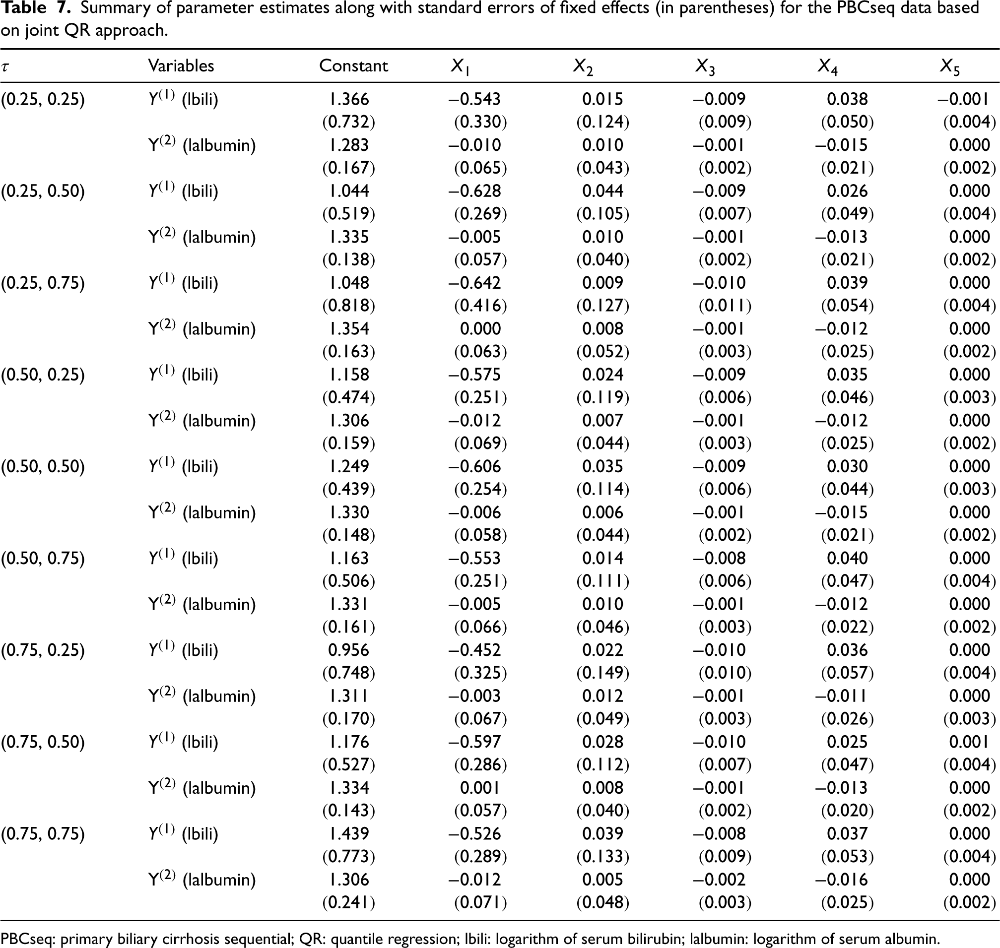
Summary of parameter estimates along with standard errors of fixed effects (in parentheses) for the PBCseq data based on joint QR approach.

$τ$	Variables	Constant	X ₁	X ₂	X ₃	X ₄	X ₅
(0.25, 0.25)	$Y^{(1)}$ (lbili)	1.366	−0.543	0.015	−0.009	0.038	−0.001
		(0.732)	(0.330)	(0.124)	(0.009)	(0.050)	(0.004)
	$Y^{(2)}$ (lalbumin)	1.283	−0.010	0.010	−0.001	−0.015	0.000
		(0.167)	(0.065)	(0.043)	(0.002)	(0.021)	(0.002)
(0.25, 0.50)	$Y^{(1)}$ (lbili)	1.044	−0.628	0.044	−0.009	0.026	0.000
		(0.519)	(0.269)	(0.105)	(0.007)	(0.049)	(0.004)
	$Y^{(2)}$ (lalbumin)	1.335	−0.005	0.010	−0.001	−0.013	0.000
		(0.138)	(0.057)	(0.040)	(0.002)	(0.021)	(0.002)
(0.25, 0.75)	$Y^{(1)}$ (lbili)	1.048	−0.642	0.009	−0.010	0.039	0.000
		(0.818)	(0.416)	(0.127)	(0.011)	(0.054)	(0.004)
	$Y^{(2)}$ (lalbumin)	1.354	0.000	0.008	−0.001	−0.012	0.000
		(0.163)	(0.063)	(0.052)	(0.003)	(0.025)	(0.002)
(0.50, 0.25)	$Y^{(1)}$ (lbili)	1.158	−0.575	0.024	−0.009	0.035	0.000
		(0.474)	(0.251)	(0.119)	(0.006)	(0.046)	(0.003)
	$Y^{(2)}$ (lalbumin)	1.306	−0.012	0.007	−0.001	−0.012	0.000
		(0.159)	(0.069)	(0.044)	(0.003)	(0.025)	(0.002)
(0.50, 0.50)	$Y^{(1)}$ (lbili)	1.249	−0.606	0.035	−0.009	0.030	0.000
		(0.439)	(0.254)	(0.114)	(0.006)	(0.044)	(0.003)
	$Y^{(2)}$ (lalbumin)	1.330	−0.006	0.006	−0.001	−0.015	0.000
		(0.148)	(0.058)	(0.044)	(0.002)	(0.021)	(0.002)
(0.50, 0.75)	$Y^{(1)}$ (lbili)	1.163	−0.553	0.014	−0.008	0.040	0.000
		(0.506)	(0.251)	(0.111)	(0.006)	(0.047)	(0.004)
	$Y^{(2)}$ (lalbumin)	1.331	−0.005	0.010	−0.001	−0.012	0.000
		(0.161)	(0.066)	(0.046)	(0.003)	(0.022)	(0.002)
(0.75, 0.25)	$Y^{(1)}$ (lbili)	0.956	−0.452	0.022	−0.010	0.036	0.000
		(0.748)	(0.325)	(0.149)	(0.010)	(0.057)	(0.004)
	$Y^{(2)}$ (lalbumin)	1.311	−0.003	0.012	−0.001	−0.011	0.000
		(0.170)	(0.067)	(0.049)	(0.003)	(0.026)	(0.003)
(0.75, 0.50)	$Y^{(1)}$ (lbili)	1.176	−0.597	0.028	−0.010	0.025	0.001
		(0.527)	(0.286)	(0.112)	(0.007)	(0.047)	(0.004)
	$Y^{(2)}$ (lalbumin)	1.334	0.001	0.008	−0.001	−0.013	0.000
		(0.143)	(0.057)	(0.040)	(0.002)	(0.020)	(0.002)
(0.75, 0.75)	$Y^{(1)}$ (lbili)	1.439	−0.526	0.039	−0.008	0.037	0.000
		(0.773)	(0.289)	(0.133)	(0.009)	(0.053)	(0.004)
	$Y^{(2)}$ (lalbumin)	1.306	−0.012	0.005	−0.002	−0.016	0.000
		(0.241)	(0.071)	(0.048)	(0.003)	(0.025)	(0.002)

PBCseq: primary biliary cirrhosis sequential; QR: quantile regression; lbili: logarithm of serum bilirubin; lalbumin: logarithm of serum albumin.

Table 8.

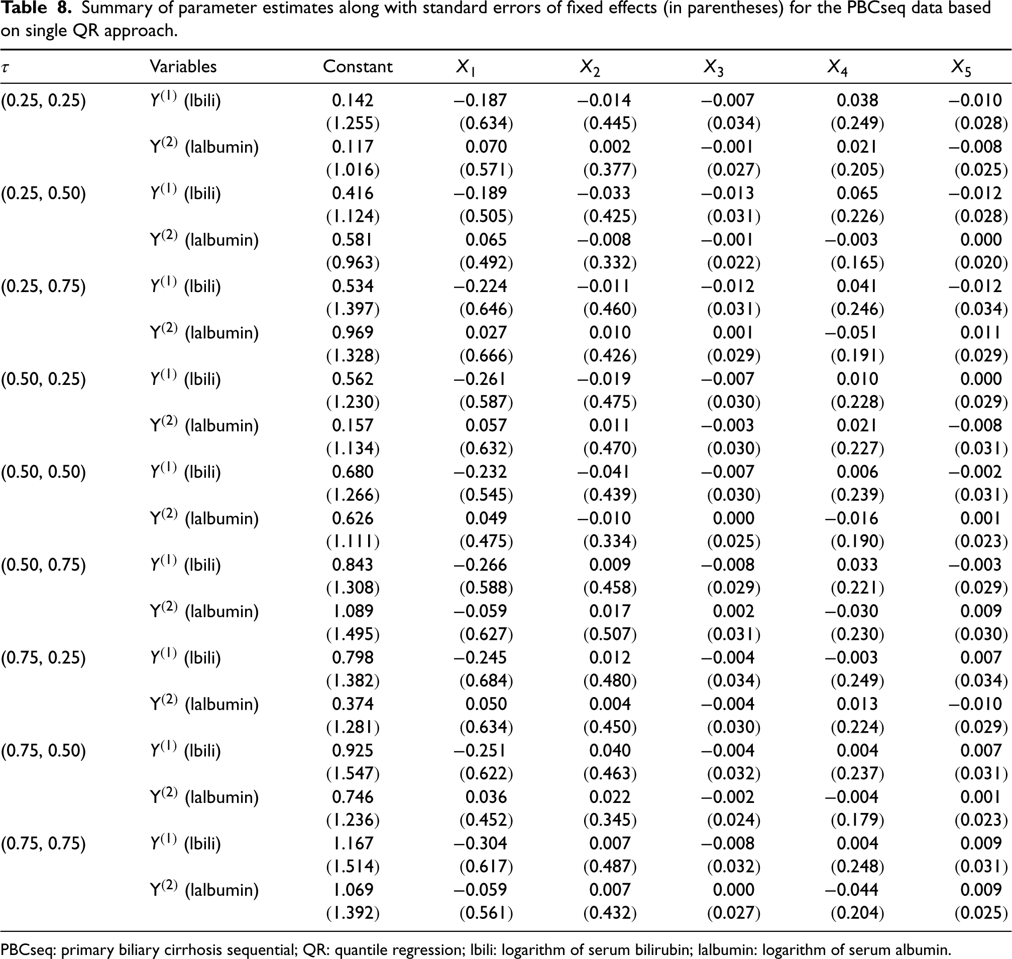
Summary of parameter estimates along with standard errors of fixed effects (in parentheses) for the PBCseq data based on single QR approach.

$τ$	Variables	Constant	X ₁	X ₂	X ₃	X ₄	X ₅
(0.25, 0.25)	$Y^{(1)}$ (lbili)	0.142	−0.187	−0.014	−0.007	0.038	−0.010
		(1.255)	(0.634)	(0.445)	(0.034)	(0.249)	(0.028)
	$Y^{(2)}$ (lalbumin)	0.117	0.070	0.002	−0.001	0.021	−0.008
		(1.016)	(0.571)	(0.377)	(0.027)	(0.205)	(0.025)
(0.25, 0.50)	$Y^{(1)}$ (lbili)	0.416	−0.189	−0.033	−0.013	0.065	−0.012
		(1.124)	(0.505)	(0.425)	(0.031)	(0.226)	(0.028)
	$Y^{(2)}$ (lalbumin)	0.581	0.065	−0.008	−0.001	−0.003	0.000
		(0.963)	(0.492)	(0.332)	(0.022)	(0.165)	(0.020)
(0.25, 0.75)	$Y^{(1)}$ (lbili)	0.534	−0.224	−0.011	−0.012	0.041	−0.012
		(1.397)	(0.646)	(0.460)	(0.031)	(0.246)	(0.034)
	$Y^{(2)}$ (lalbumin)	0.969	0.027	0.010	0.001	−0.051	0.011
		(1.328)	(0.666)	(0.426)	(0.029)	(0.191)	(0.029)
(0.50, 0.25)	$Y^{(1)}$ (lbili)	0.562	−0.261	−0.019	−0.007	0.010	0.000
		(1.230)	(0.587)	(0.475)	(0.030)	(0.228)	(0.029)
	$Y^{(2)}$ (lalbumin)	0.157	0.057	0.011	−0.003	0.021	−0.008
		(1.134)	(0.632)	(0.470)	(0.030)	(0.227)	(0.031)
(0.50, 0.50)	$Y^{(1)}$ (lbili)	0.680	−0.232	−0.041	−0.007	0.006	−0.002
		(1.266)	(0.545)	(0.439)	(0.030)	(0.239)	(0.031)
	$Y^{(2)}$ (lalbumin)	0.626	0.049	−0.010	0.000	−0.016	0.001
		(1.111)	(0.475)	(0.334)	(0.025)	(0.190)	(0.023)
(0.50, 0.75)	$Y^{(1)}$ (lbili)	0.843	−0.266	0.009	−0.008	0.033	−0.003
		(1.308)	(0.588)	(0.458)	(0.029)	(0.221)	(0.029)
	$Y^{(2)}$ (lalbumin)	1.089	−0.059	0.017	0.002	−0.030	0.009
		(1.495)	(0.627)	(0.507)	(0.031)	(0.230)	(0.030)
(0.75, 0.25)	$Y^{(1)}$ (lbili)	0.798	−0.245	0.012	−0.004	−0.003	0.007
		(1.382)	(0.684)	(0.480)	(0.034)	(0.249)	(0.034)
	$Y^{(2)}$ (lalbumin)	0.374	0.050	0.004	−0.004	0.013	−0.010
		(1.281)	(0.634)	(0.450)	(0.030)	(0.224)	(0.029)
(0.75, 0.50)	$Y^{(1)}$ (lbili)	0.925	−0.251	0.040	−0.004	0.004	0.007
		(1.547)	(0.622)	(0.463)	(0.032)	(0.237)	(0.031)
	$Y^{(2)}$ (lalbumin)	0.746	0.036	0.022	−0.002	−0.004	0.001
		(1.236)	(0.452)	(0.345)	(0.024)	(0.179)	(0.023)
(0.75, 0.75)	$Y^{(1)}$ (lbili)	1.167	−0.304	0.007	−0.008	0.004	0.009
		(1.514)	(0.617)	(0.487)	(0.032)	(0.248)	(0.031)
	$Y^{(2)}$ (lalbumin)	1.069	−0.059	0.007	0.000	−0.044	0.009
		(1.392)	(0.561)	(0.432)	(0.027)	(0.204)	(0.025)

PBCseq: primary biliary cirrhosis sequential; QR: quantile regression; lbili: logarithm of serum bilirubin; lalbumin: logarithm of serum albumin.

We concentrate on modeling the dependence of the longitudinal profiles of two markers with the natural logarithm of serum bilirubin (lbili) and the natural logarithm of serum albumin (lalbumin), on time (visited years) and other covariates of interest (e.g. sex, drug, and age). We conduct the joint QR analysis for the longitudinal PBCseq data set on responses of lbili and lalbumin by establishing model (3.1). Denote $y_{i t} = (y_{i t}^{(1)}, y_{i t}^{(2)})^{T}, x_{i t} = (1, x_{i t 1}, x_{i t 2}, x_{i t 3}, x_{i t 4}, x_{i t 5})^{T}, i \in 1, \dots, 312$ , where $y_{i t}$ is the bivariate response for the $i$ -th patient, $y_{i t}^{(1)}$ and $y_{i t}^{(2)}$ represent lbili and lalbumin levels, and $x_{i t}$ is a $6 \times 1$ vector of regressors, $x_{i t 1} (gender)$ denotes the gender indicator (0 = male and 1 = female), $x_{i t 2} (drug)$ denotes the drug treatment indicator (0 = patient treated with placebo and 1 = patient treated with D-penicillamine), $x_{i t 3} (age)$ denotes the age at entry in years, $x_{i t 4} (month / 12)$ denotes time (visited years), and $x_{i t 5} = x_{i t 4}^{2}$ . Thus, the parameter matrix of fixed effects is denoted as

\begin{aligned} β_{2 \times 5} = (\begin{array}{llllll} β_{10} & β_{11} & β_{12} & β_{13} & β_{14} & β_{15} \\ β_{20} & β_{21} & β_{22} & β_{23} & β_{24} & β_{25} \end{array}) \end{aligned}

Nine quantile combinations, that is,

τ = (0.25, 0.25)

τ = (0.25, 0.55)

τ = (0.25, 0.75)

τ = (0.50, 0.25)

τ = (0.50, 0.50)

τ = (0.50, 0.75)

τ = (0.75, 0.25)

τ = (0.75, 0.50)

, and

τ = (0.75, 0.75)

, are considered for the response

(y_{i t}^{(1)}, y_{i t}^{(2)})^{T}

. The priors and initial values are set as the same setting in Section 5. We run

8000

iterations of Gibbs sampling algorithm for each quantile combination, the first 2000 burn-in iterations are removed and the remaining 6000 stationary iterations are retained to conduct posterior inference. Estimation results including average estimation values and standard errors of the considered nine quantile combinations are reported in Table 7. For the aim of comparison, we also provide the estimation results of single QR approach in Table 8.

Compared Table 7 with Table 8, we again conclude that the proposed joint QR approach has better estimation results with apparently smaller standard errors for almost all parameters. In addition, from Table 7, we find that five covaraites have not exactly the same impacts on two responses for each quantile combination. The impacts of five covariates on two responses also totally vary with the quantile combinations. Further, at all quantile levels under consideration, covariates $X_{1}$ (gender) and $X_{3}$ (age) have simultaneous negative effects on responses $Y_{1}$ (lbili) and $Y_{2}$ (lalbumin), and covariates $X_{2}$ (drug) have simultaneous positive effects on two responses. Yet, $X_{1}$ has a clearly bigger impact on response $Y_{1}$ than $Y_{2}$ while $X_{2}$ has a slightly bigger impact on response $Y_{1}$ than $Y_{2}$ . Whereas, covariates $X_{4}$ (visited years) has positive effects on response $Y_{1}$ and negative effects on response $Y_{2}$ for all quantiles. Specially, we find $X_{5}$ has almost no impact on responses $Y_{1}$ and $Y_{2}$ for all considered quantiles since the coefficients are approximately estimated as zeros. Some useful conclusions can be drawn based on the above quantitative analysis. lbili and lalbumin becomes slightly smaller as the ages of patients increase. Female patients ( $X_{1} = 1$ ) have faster change for lbili and lalbumin than male patients ( $X_{1} = 0$ ). Patients treated with D-penicillamine ( $X_{2} = 1$ ) have bigger change for lbili and lalbumin than patients treated with placebo ( $X_{2} = 0$ ). Generally, in the diagnosis of clinical liver disease patients, the increase of serum bilirubin and the decrease of serum albumin indicate liver cell damage. Hence, conclusions suggest elderly female patients with liver disease more should receive medication intervention of D-penicillamine to more effectively reduce the risk of liver disease development.

7. Concluding remarks

We investigated the Bayesian joint QR modeling of multi-response mixed-effects model with longitudinal data in this paper. A MAL distribution was imposed on the errors of the considered model to build the working likelihood of Bayesian joint inference. For implementing the efficient Bayesian inference, the location-scale mixture reparameterization of the working likelihood and LASSO-type penalization priors of regression coefficients were employed to construct the Bayesian joint hierarchical QR model. The conditional posterior distributions of parameters and latent variables based on MCMC algorithm were derived. Monte Carlo simulation examples were presented to illustrate the proposed joint QR approach. Simulation results showed that the proposed joint QR approach has more satisfactory performance than the single QR approach. Finally, we analyzed a real-world data set of a longitudinal PBCseq cohort study using the proposed joint modeling approach. The proposed joint QR approach can be extended to more complex longitudinal data models and applications.

Footnotes

Acknowledgements

The authors thank editors and two referees for their constructive comments and suggestions which have greatly improved the paper. The work of Tian Yu-Zhu was jointly supported by grants from the National Natural Science Foundation of China (Grant 12061065) and Funds for Innovative Fundamental Research Group Project of Gansu Province of China (Grant 23JRRA684). The work of Tang Man-Lai is partially supported by the Research Matching Grant (700006) from the Research Grants Council of the Hong Kong Special Administration Region and FDS Grant (UGC/FDS14/P05/20) from the Big Data Intelligence Center in The Hang Seng University of Hong Kong.

Declaration of conflicting interests

The author(s) declared no potential conflicts of interest with respect to the research, authorship, and/or publication of this article.

ORCID iD

Catherine Wong

Supplemental material

Supplemental material for this article is available online.

References

Laird

Ware

. Random-effect models for longitudinal data. Biometrics 1982; 38: 963–974.

Diggle

Heagerty

Liang

, et al. Analysis of longitudinal data. USA: Oxford University Press, 2002.

Hedeker

Gibbons

. Longitudinal data analysis. Wiley, New Jersey: Blackwell Publishing Ltd, 2006.

Zhang

. Nonparametric regression methods for longitudinal data analysis: mixed-effects modeling approaches. New York: Wiley, 2006.

. Mixed effects models for complex data. Boca Raton: Chapman & Hall/CRC Press, 2010.

Demidenko

. Mixed Models: Theory and Applications with R. (2nd ed). Hoboken Wiley, 2013.

Shah

Laird

Schoenfeld

. A random-effects model for multiple characteristics with possibly missing data. J Am Stat Assoc 1997; 438: 775–779.

Sammel

Lin

Ryan

. Multivariate linear mixed models for multiple outcomes. Stat Med 1999; 18: 2479–2492.

Lin

. A mixed-effects regression model for longitudinal multivariate ordinal data. Int Biometric Soc 2006; 62: 261–268.

10.

Blozis

Conger

Harring

. Nonlinear latent curve models for multivariate longitudinal data. Int J Behav Dev 2007; 31: 340–346.

11.

Alfo

Maruotti

. A hierarchical model for time dependent multivariate longitudinal data. Berlin, Heidelberg: Springer, 2010.

12.

Bandyopadhyay

Ganguli

Chatterjee

. A review of multivariate longitudinal data analysis. Stat Methods Med Res 2011; 20: 299–330.

13.

Gebregziabher

Zhao

Dismuke

, etc. Joint modeling of multiple longitudinal cost outcomes using multivariate generalized linear mixed models. Health Serv Outc Res Methodol 2013; 13: 39–57.

14.

Laffont

Vandemeulebroecke

Concordet

. Multivariate analysis of longitudinal ordinal data with mixed effects models, with application to clinical outcomes in osteoarthritis. J Am Stat Assoc 2014; 109: 955–966.

15.

Grimm

. Multivariate longitudinal methods for studying developmental relationships between depression and academic achievement. Int J Behav Dev 2015; 31: 328–339.

16.

Wang

Lin

Lachos

. Extending multivariate-t linear mixed models for multiple longitudinal data with censored responses and heavy tails. Stat Methods Med Res 2015; 27: 48–64.

17.

Luwanda

Mwambi

. A nonlinear mixed-effects model for multivariate longitudinal data with partially observed outcomes with application to HIV disease dynamics. J Appl Stat 2017; 44: 441–456.

18.

Rajeswaran

Blackstone

Barnard

. Joint modeling of multivariate longitudinal data and competing risks using multiphase sub-models. Stat Biosci 2018; 10: 651–685.

19.

Lin

Lachos

Wang

. Multivariate longitudinal data analysis with censored and intermittent missing responses. Stat Med 2018; 37: 2822–2835.

20.

Hui

FKC

Mueller

Welsh

. Sparse pairwise likelihood estimation for multivariate longitudinal mixed models. J Am Stat Assoc 2018; 113: 1759–1769.

21.

Jiang

Yue

Zhou

. Optimal designs for multivariate logistic mixed models with longitudinal data. Commun Stat-Theory Method 2019; 48: 850–864.

22.

Wang

. Bayesian analysis of multivariate linear mixed models with censored and intermittent missing responses. Stat Med 2020; 39: 2518–2535.

23.

Taavoni

Arashi

Wang

, et al. Multivariate

t

semiparametric mixed-effects model for longitudinal data with multiple characteristics. J Stat Comput Simul 2021; 91: 260–281.

24.

Tian

Qiu

. Multivariate single index modeling of longitudinal data with multiple responses. Stat Med 2023; 42: 2982–2998.

25.

Koenker

. Quantile regression. Cambridge: Cambridge University Press, 2005.

26.

Koenker

Chernozhukov

, et al. Handbook of Quantile Regression. Florida CRC Press, 2017.

27.

Koenker

. Quantile regression for longitudinal data. J Multivar Anal 2004; 91: 74–89.

28.

Geraci

Bottai

. Quantile regression for longitudinal data using the asymmetric Laplace distribution. Biostatistics 2007; 8: 140–154.

29.

Liu

Bottai

. Mixed-effects models for conditional quantiles with longitudinal data. Int J Biostat 2009; 5: 1–24.

30.

Tian

. Bayesian joint quantile regression for mixed effects models with censoring and errors in covariates. Comp Stat 2016; 31: 1–27.

31.

Aghamohammadi

Mohammadi

. Bayesian analysis of penalized quantile regression for longitudinal data. Stat Pap 2017; 58: 1035–1053.

32.

Alhamzawi

Ali

HTM

. Bayesian quantile regression for ordinal longitudinal data. J Appl Stat 2018; 45: 815–828.

33.

Tian

Wang

Tang

, et al. Likelihood-based quantile mixed effects models for longitudinal data with multiple features via MCEM algorithm. Commun Stat-Simul Comput 2020; 49: 317–334.

34.

Waldmann

Kneib

. Bayesian bivariate quantile regression. Stat Model 2014; 15: 326–344.

35.

Kulkarni

Biswas

Das

. A joint quantile regression model for multiple longitudinal outcomes. AStA-Adv Stat Anal 2019; 103: 453–473.

36.

Ghasemzadeh

Ganjali

Baghfalaki

. Bayesian quantile regression for joint modeling of longitudinal mixed ordinal and continuous data. Commun Stat Simul Comput 2020; 49: 375–395.

37.

Biswas

Das

. A Bayesian quantile regression approach to multivariate semi-continuous longitudinal data. Comput Stat 2021; 36: 241–260.

38.

Petrella

Raponi

. Joint estimation of conditional quantiles in multivariate linear regression models with an application to financial distress. J Multivar Anal 2019; 173: 70–84.

39.

Tian

Tang

Tian

. Bayesian joint inference for multivariate quantile regression model with

L_{1 / 2}

penalty. Comput Stat 2021; 36: 2967–2994.

40.

Kotz

Kozubowski

. Symmetric multivariate Laplace distribution. Asymmetric multivariate Laplace distribution. Boston, MA: Springer, 2001.

41.

Kollo

Srivastava

. Estimation and testing of parameters in multivariate Laplace distribution. Commun Stat-Theory Method 2005; 33: 2363–2387.

42.

Visk

. On the parameter estimation of the asymmetric multivariate Laplace distribution. Commun Stat-Theory Method 2009; 38: 461–470.

43.

Hurlimann

. A moment method for the multivariate asymmetric Laplace distribution. Stat Probab Lett 2013; 83: 1247–1253.

44.

Tibshirani

. Regression shrinkage and selection via the LASSO. J R Stat Soc (Ser B) 1996; 73: 273–282.

45.

Zou

. The adaptive LASSO and its oracle properties. J Am Stat Assoc 2006; 101: 1418–1429.

46.

Park

Casella

. The Bayesian LASSO. J Am Stat Assoc 2008; 103: 681–686.

47.

Leng

Tran

Nott

. Bayesian adaptive LASSO. Ann Inst Stat Math 2014; 66: 221–244.

48.

Fukui

Tanaka

Shiraishi

, et al. Relationship between serum bilirubin and albuminuria in patients with type 2 diabetes. Kidney Int 2008; 74: 1197–1201.

49.

Komarek

Komarkova

. Capabilities of R package mixAK for clustering based on multivariate continuous and discrete longitudinal data. J Stat Softw 2014; 59: 1–38.

50.

Wang

. Mixture of multivariate

t

linear mixed models for multi-outcome longitudinal data with heterogeneity. Stat Sin 2017; 27: 733–760.

Bayesian analysis of joint quantile regression for multi-response longitudinal data with application to primary biliary cirrhosis sequential cohort study

Abstract

Keywords

1. Introduction

2. Preliminaries

3.1. The multi-response longitudinal mixed-effect model

4.1. Prior specifications

Table 7. Summary of parameter estimates along with standard errors of fixed effects (in parentheses) for the PBCseq data based on joint QR approach.

Footnotes

Acknowledgements

Declaration of conflicting interests

ORCID iD

Supplemental material

References

Table 7.
Summary of parameter estimates along with standard errors of fixed effects (in parentheses) for the PBCseq data based on joint QR approach.