
Abstract
In medical and health research, investigators are often interested in countable quantities such as hospital length of stay (e.g., in days) or the number of doctor visits. Poisson regression is commonly used to model such count data, but this approach can’t accommodate overdispersion—when the variance exceeds the mean. To address this issue, the negative binomial (NB) distribution (NB-D) and, by extension, NB regression provide a well-documented alternative. However, real-data applications present additional challenges that must be considered. Two such challenges are (i) the presence of (mild) outliers that can influence the performance of the NB-D and (ii) the availability of covariates that can enhance inference about the mean of the count variable of interest. To jointly address these issues, we propose the contaminated NB (cNB) distribution that exhibits the necessary flexibility to accommodate mild outliers. This model is shown to be simple and intuitive in interpretation. In addition to the parameters of the NB-D, our proposed model has a parameter describing the proportion of mild outliers and one specifying the degree of contamination. To allow available covariates to improve the estimation of the mean of the cNB distribution, we propose the cNB regression model. An expectation-maximization algorithm is outlined for parameter estimation, and its performance is evaluated through a parameter recovery study. The effectiveness of our model is demonstrated via a sensitivity analysis and on two health datasets, where it outperforms well-known count models. The methodology proposed is implemented in an
Introduction
Count data are routinely encountered across various disciplines including epidemiology, social sciences, and economics1,2; particularly noteworthy is their prevalence in the realm of healthcare and medicine.3–5 Investigators are often interested in countable quantities such as hospital length of stay (e.g. in days) or the number of doctor visits. Length of stay is often used as an indicator of efficiency, as a shorter stay will reduce the cost per discharge and shift care from inpatient to less expensive post-acute settings.6,7 Likewise, the number of doctor visits serves as a measure of healthcare utilization and access, reflecting the frequency and necessity of medical care received by patients. 8 Analyzing these metrics helps assess the overall performance and efficiency of healthcare systems, understand patient behavior and needs, and identify areas for potential improvement in service delivery and cost management.
The values of the count variables are always nonnegative integers, and the distribution is often skewed. The Poisson regression model (Poisson-RM) is traditionally the first considered method for such data and implies a Poisson assumption for the counts conditional to some covariates. However, it operates under the assumption that the conditional mean and variance of the counts are equal. This drawback limits its applicability in scenarios where overdispersion or “extra-Poisson” variation is evident.9–12
As discussed by Hilbe,
13
there are two types of overdispersion: apparent and real. Apparent overdispersion can be remedied by various operations on the data, such as adding appropriate predictor(s), constructing required interactions, and transforming predictor(s) or the response. Conversely, real overdispersion is a problem that affects the reliability of both the model parameter estimates and fit in general. To address the shortcomings of the Poisson distribution (Pois-D) in the presence of real overdispersion, the negative binomial (NB) distribution (NB-D) has emerged as a viable alternative. The probability mass function (PMF) of the mean parameterized NB-D for a count variable


As discussed by Hilbe, 13 even though the NB-D alleviates the highly restrictive assumption of equidispersion posed by the Pois-D, there are instances where NB-Ds may also be overdispersed. While Poisson overdispersion occurs when its observed distributional variance exceeds the mean, NB overdispersion occurs when the calculated model variance exceeds the nominal NB variance. The NB-D may, therefore, be inadequate in modeling the variance inherent in the data. It is thus possible that both Poisson and NB overdispersions might occur at the same time.
While one common cause of overdispersion is excess zeros by an additional data-generating process, another contributing factor to larger variances, and thus possible overdispersion, is the presence of outliers in the data. 13 As discussed by Ritter, 15 real-world data is often contaminated with outliers or atypical observations that can affect the estimation of model parameters, or in the context of regression, the regression coefficients. Inappropriate imposition of the Pois-D and NB-D may underestimate the standard errors and overstate the significance of the regression coefficients, which could lead to misleading inference.
This raises the question: How should outliers be handled? To answer this, it is important to note that outliers are generally divided into two broad categories:
Mild outliers: Observations sampled from some population different or even far from the assumed model. Gross outliers: Observations that cannot be modeled by a distribution as they are unpredictable.
In the presence of gross outliers, the recommended approach is to eliminate the observations or choose a suitable method for suppressing them.
16
For mild outliers, however, it is usually recommended to use a model flexible enough to accommodate the atypical data points,15,17 which is of specific interest in this article. We propose the contaminated NB distribution (cNB-D) on which the majority of observations are from the NB-D, and the minority proportion is from an NB-D with higher dispersion. This is analogous to works presented by Mazza and Punzo,
18
Morris et al.,
19
Punzo and McNicholas,
20
Punzo and Tortora,
21
and Tomarchio et al.22,23 The resulting model is in the form of a two-component mixture, with one component representing the “good” observations (reference NB-D) and the other having the same mean but an inflated dispersion parameter, representing the “bad” observations (contaminant distribution), making it flexible enough to accommodate mild outliers. Note that both of these components have the same mean, which is the mean accounted for by the majority of the data that are considered “good”; additionally, this provides for a more parsimonious model. For a discussion on the concept of a reference distribution (which in this article is assumed to be the NB in (1)) see Davies and Gather
24
and Hennig.
25
Another issue arises when modeling the kurtosis of data. Although the excess kurtosis of
As a motivating example, Figure 1 displays data from a medical study conducted in Germany, illustrating the possible outliers in the number of doctor visits. Government spending on health care surged in Germany in the 1980s and 1990s, and, in an effort to curtail this expenditure, a major healthcare reform took place in 1997. The reform raised the co-payments by up to 200% and introduced upper limits on the reimbursement of physicians by state insurance. Patients were surveyed for the one-year panel (1996) before and the one-year panel (1998) after reform to assess whether the number of physician visits by patients declined. The dataset from the German Socio-Economic Panel 26 can be downloaded from the Journal of Applied Econometrics Data Archive. For the one-year panel of 1998 of working women, we focus on a subset of this data, as utilized by Hilbe, 13 Klakattawi et al., 27 and Yee, 28 to examine the number of doctor visits of patients who claimed to be of bad health. As illustrated in Figure 1, there seems to be an excess of points at the sides of the support (an excess of zeros on the left, and some too large values on the right) which may cause overdispersion. In this health study, mild outliers might include patients who excessively visited the doctor, much more than expected, given a model; therefore they can be considered as outliers in response to the assumed model. These outliers have the potential to introduce bias into the estimates of the regression coefficients, distort inference, and result in an overestimation of the overdispersion parameter, consequently leading to an overestimation of standard errors.
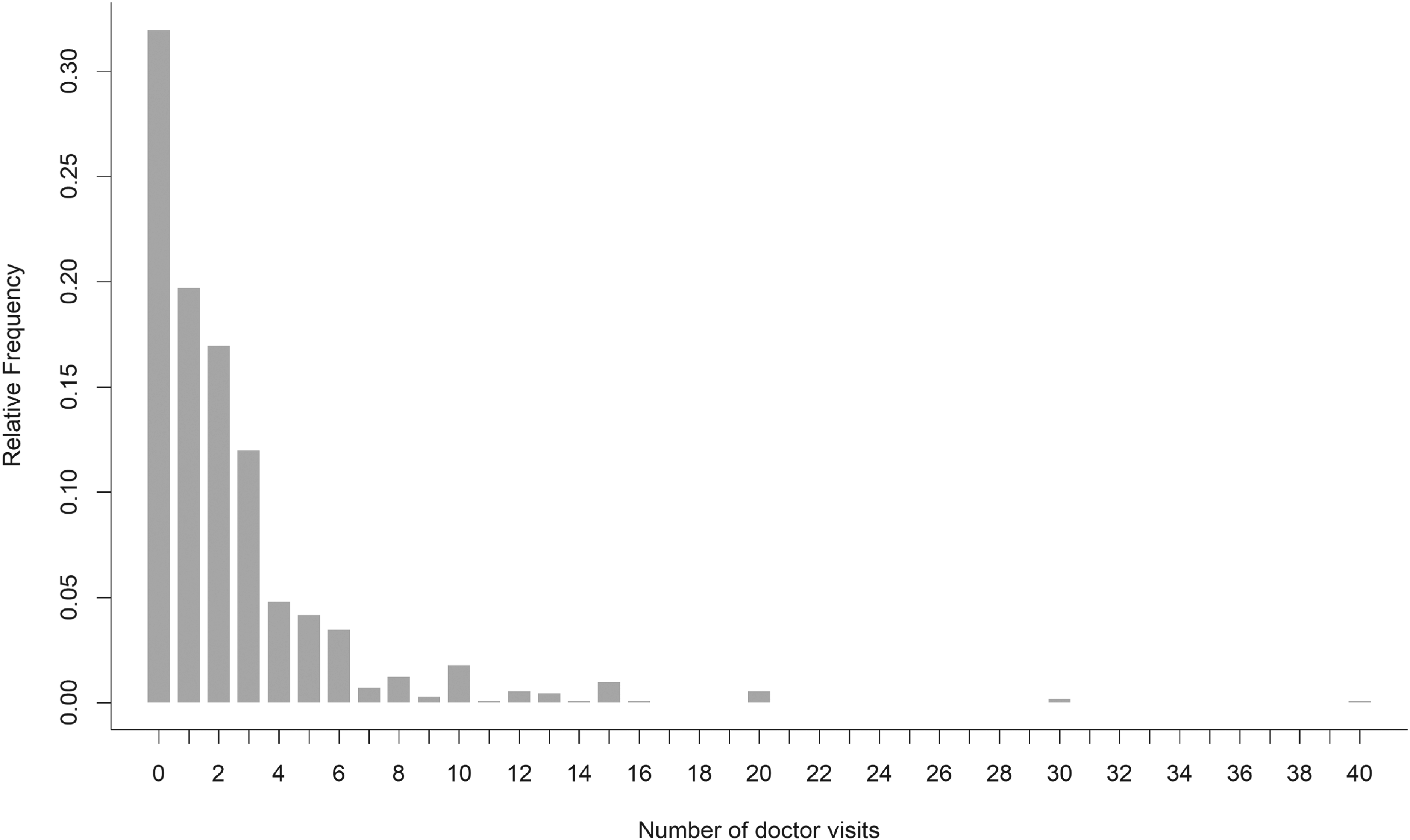
Barplot of the number of visits to a doctor in a year.
The article is set out as follows. In Section 2, we construct the cNB regression model (cNB-RM) using the proposed cNB-D in a regression context, that can capture NB overdispersion and classify whether an observation is a mild outlier once the model is fitted. The corresponding expectation-maximization (EM) algorithm for maximum likelihood (ML) estimation is presented in Section 3.2, along with a discussion of proposed initialization strategies and the convergence criteria considered in Section 3.3. A simulation study in Section 4 illustrates its parameter recovery ability, followed by a sensitivity analysis to investigate the impact of a single atypical observation on the estimations. Two real-data applications are presented in Section 5 to illustrate the viability of the cNB-D as an alternative model for overdispersed data. Finally, conclusions are drawn in Section 6.
In this section, we introduce the cNB-D (Section 2.1) and the cNB-RM (Section 2.2).
The contaminated negative binomial model
The PMF of the proposed cNB-D is

The moments of practical interest of

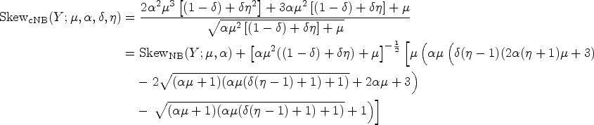


Examples illustrating the higher variance of the cNB-D (4) compared to the NB-D (1) for increasing values of
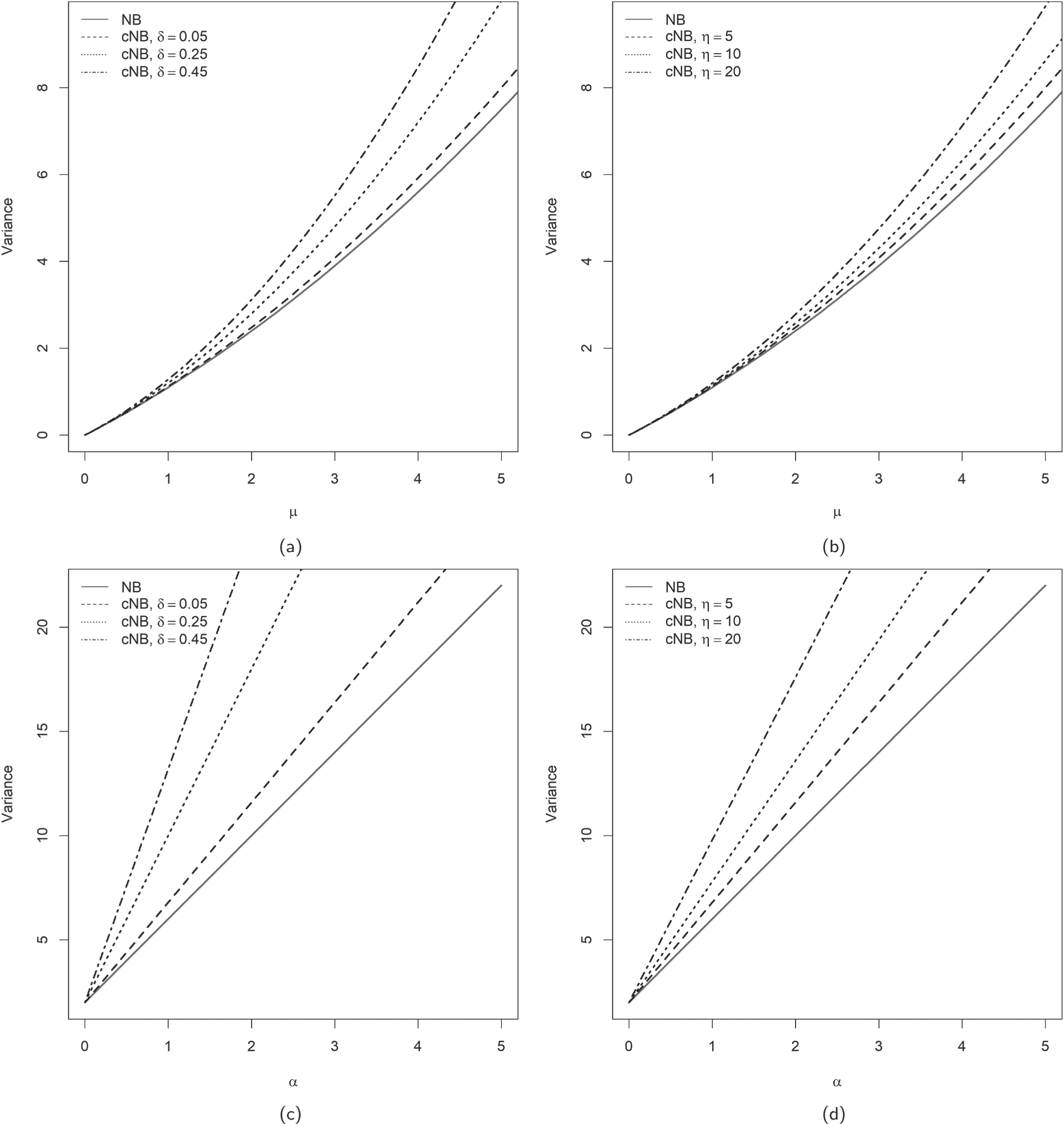
Examples illustrating higher skewness of the cNB-D (4) compared to the NB-D (1) for increasing values of
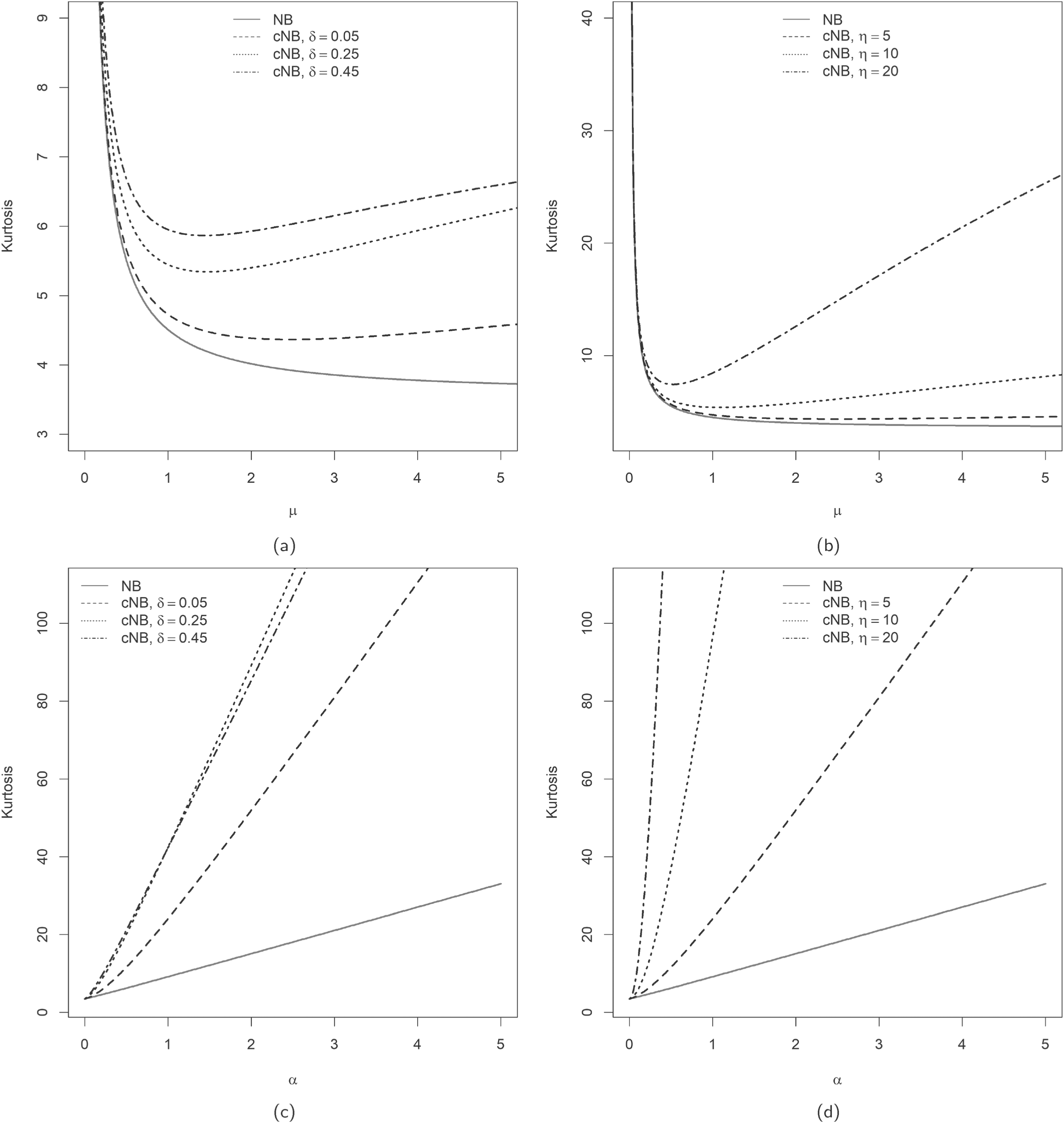
Examples illustrating higher kurtosis of the cNB-D (4) compared to the NB-D (1) for increasing values of
The following proposition explores the limiting cases of the cNB-D at the border of its parameter space.
Let if if if if
where
See Appendix A. □
A regression model based on the cNB-D (4) follows by conditioning the distribution of the count response


In this section, we discuss the identifiability of the cNB-D (Section 3.1), followed by a presentation of the EM algorithm (Section 3.2) for ML estimation of the more general cNB-RM. The initialization strategy and convergence criteria considered (Section 3.3) and an explanation of how the standard errors of the estimates are computed (Section 3.4) are also discussed.
Identifiability
Identifiability is a fundamental prerequisite for many statistical procedures, including the asymptotic theory in ML estimation of model parameters. According to Yakowitz and Spragins,
30
it is demonstrated that finite NB-mixtures are identifiable. This result is particularly relevant since the cNB-D can be viewed as a two-component NB-mixture, with both components sharing the same mean parameter
An EM algorithm
We illustrate the EM algorithm for the more general cNB-RM. Let

In the E-step, we compute the conditional expectation of the complete-data log-likelihood function as


An update

Initialization and convergence
The starting values are a critical step in EM-based algorithms and can greatly impact the accuracy and reliability of the model estimates20,31; their choice thus constitutes an important aspect of estimation. If the starting values are chosen poorly, the algorithm may converge to a local maximum instead of the global maximum. Moreover, if the starting values deviate too much from the true values, the algorithm may converge slowly or not at all. We suggest fitting a standard NB-RM using the same predictors that would be used to fit a cNB-RM to the data. The estimated coefficients can then serve as initial values for fitting a cNB-RM. For
As for the stopping rule, there are several convergence criteria that can be used to determine whether the EM algorithm has converged or not. One common method is to track the change in the observed-data log-likelihood function, say
Standard errors of the estimates
After executing the EM algorithm described in Section 3.2, the variance-covariance matrix of the parameter estimates is obtained by inverting the negative Hessian matrix, computed using the
Simulation studies
In this section, various aspects related to the proposed cNB-RM are investigated. We only focus on the cNB-RM because it is more general than the cNB-D. As the EM algorithm is used to fit the model, assessing its performance in terms of parameter recovery is imperative. The results of a parameter recovery study are presented in Section 4.1, while a sensitivity analysis that aims to evaluate the influence of a single outlier on the parameter estimates of the NB-RM and cNB-RM is illustrated in Section 4.2. The ability of the cNB-RM to determine whether an observation is “good” or “bad,” as given in (8), is also evaluated.
Parameter recovery
Parameter recovery focuses on the algorithm’s ability to accurately retrieve the true generating parameters. If, across multiple replications, the mean of the estimates significantly deviates from the actual generating parameter, the estimator is deemed biased. Additionally, the extent of variability in the estimates across these replications is a matter of concern. With small to moderate sample sizes, the ML estimator of the dispersion parameter may be subject to significant bias, which, in turn, may affect the coefficient estimates.
32
The bias may even be more pronounced in the case of the cNB-D. If only a few mild outliers are in the sample, this could lead to sparse data for the contaminated component in (4) leading to numerical instabilities in
As described by Hilbe,
13
the NB-D is typically derived as a Poisson-gamma mixture. Although this result can be exploited in the generation of NB data, we directly used the
We simulate cNB-RM with cNB-RM with
with an intercept of
Parameter recovery results for Scenario 1 with an intercept of
, a binary covariate with coefficient
, and a continuous covariate with coefficient
,
and
for different values of
, based on
replications of varying sample sizes.

Parameter recovery results for Scenario 1 with an intercept of
MSE: mean squared error.
Parameter recovery results for Scenario 2 with an intercept of
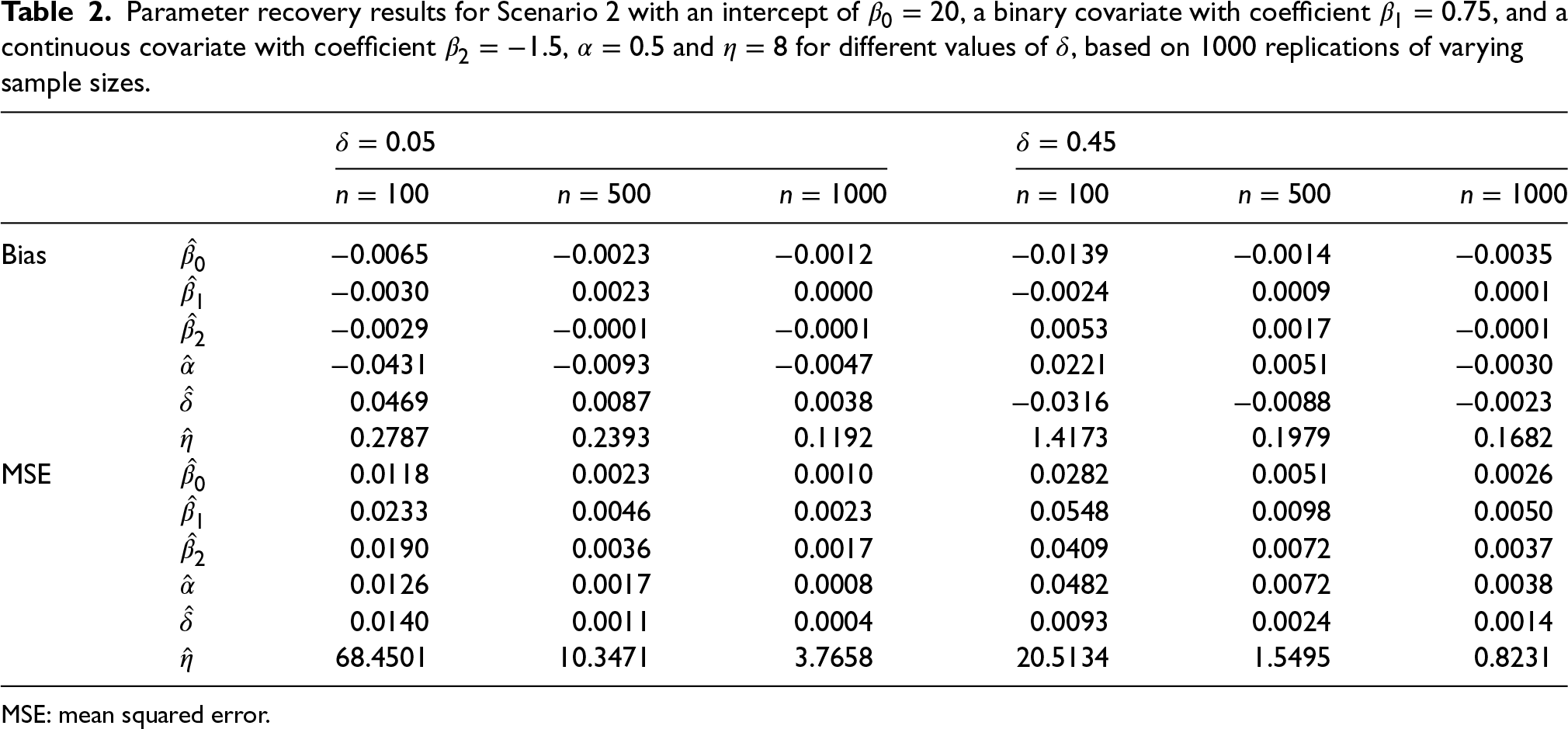
MSE: mean squared error.
In the various scenarios investigated, we observe accurate parameter recovery and note that an increase in sample size leads to reduced bias, variability, and consequently MSE, within these estimates. The estimation of the regression coefficients is nearly perfect across all the data configurations. Instead,
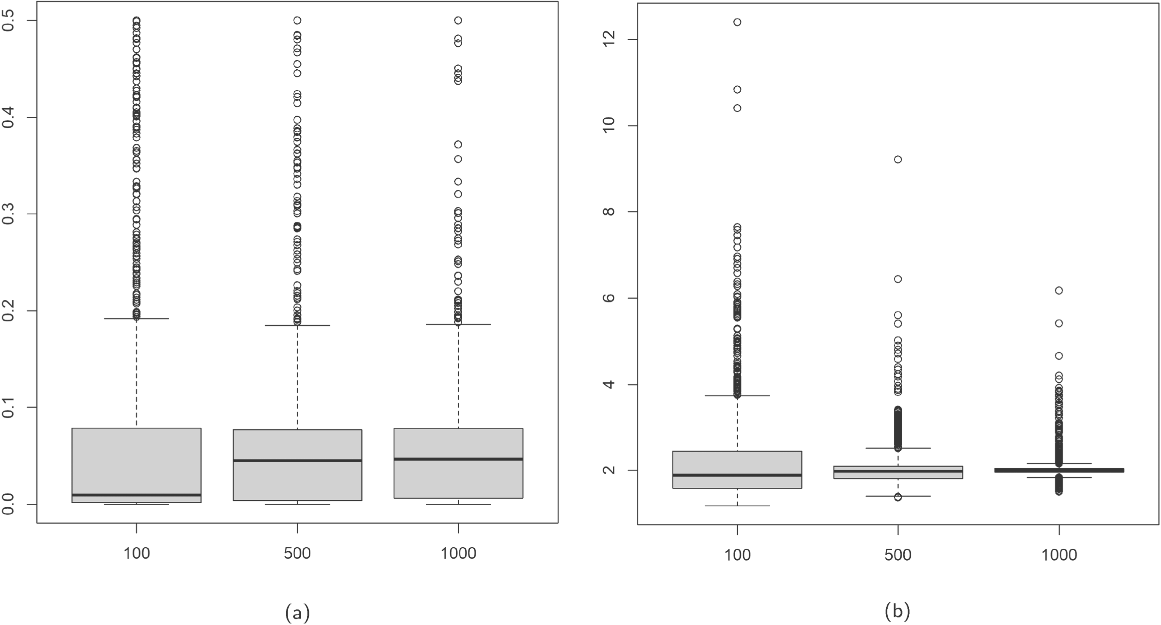
Boxplot of
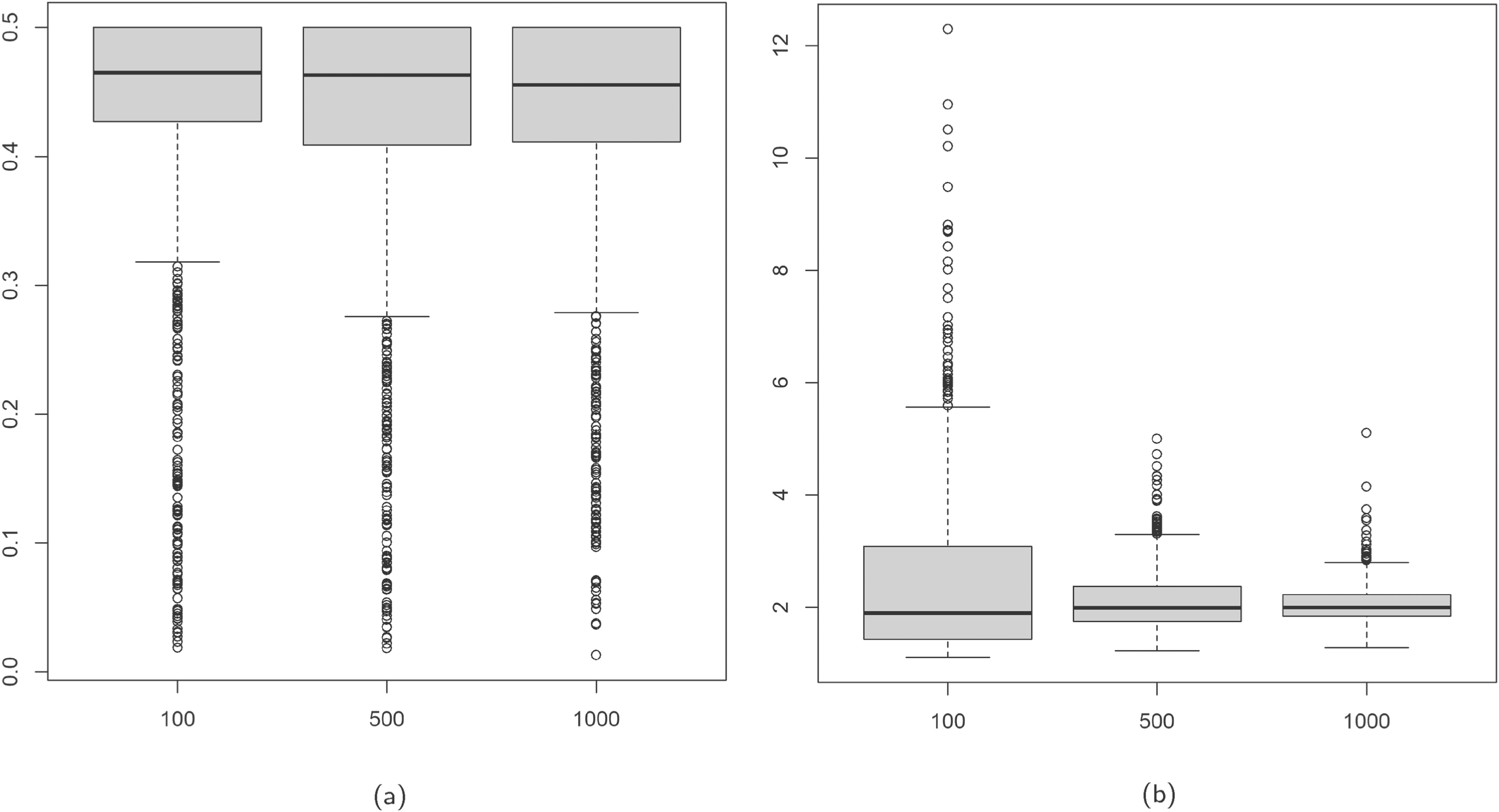
Boxplots of
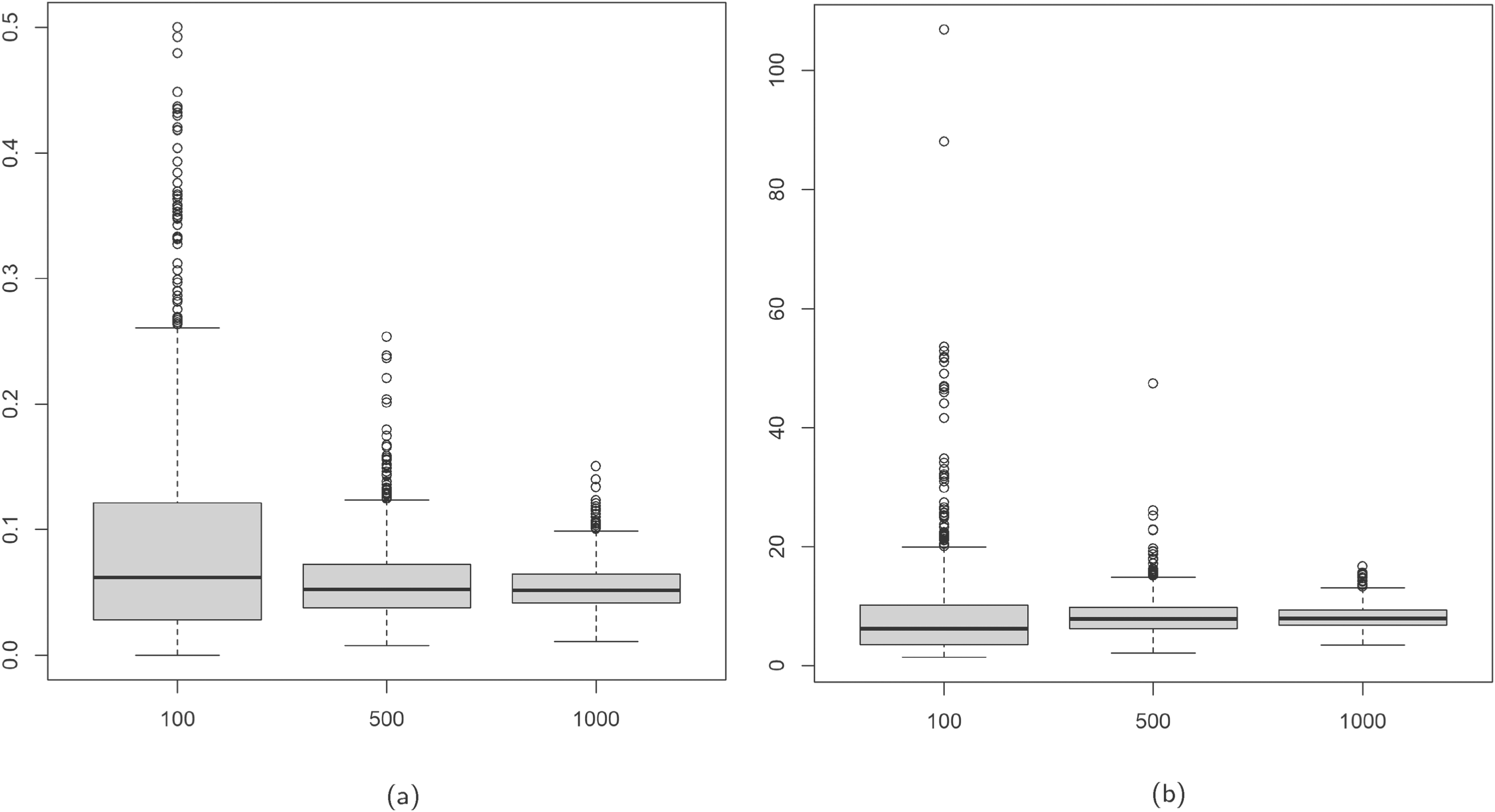
Boxplots of
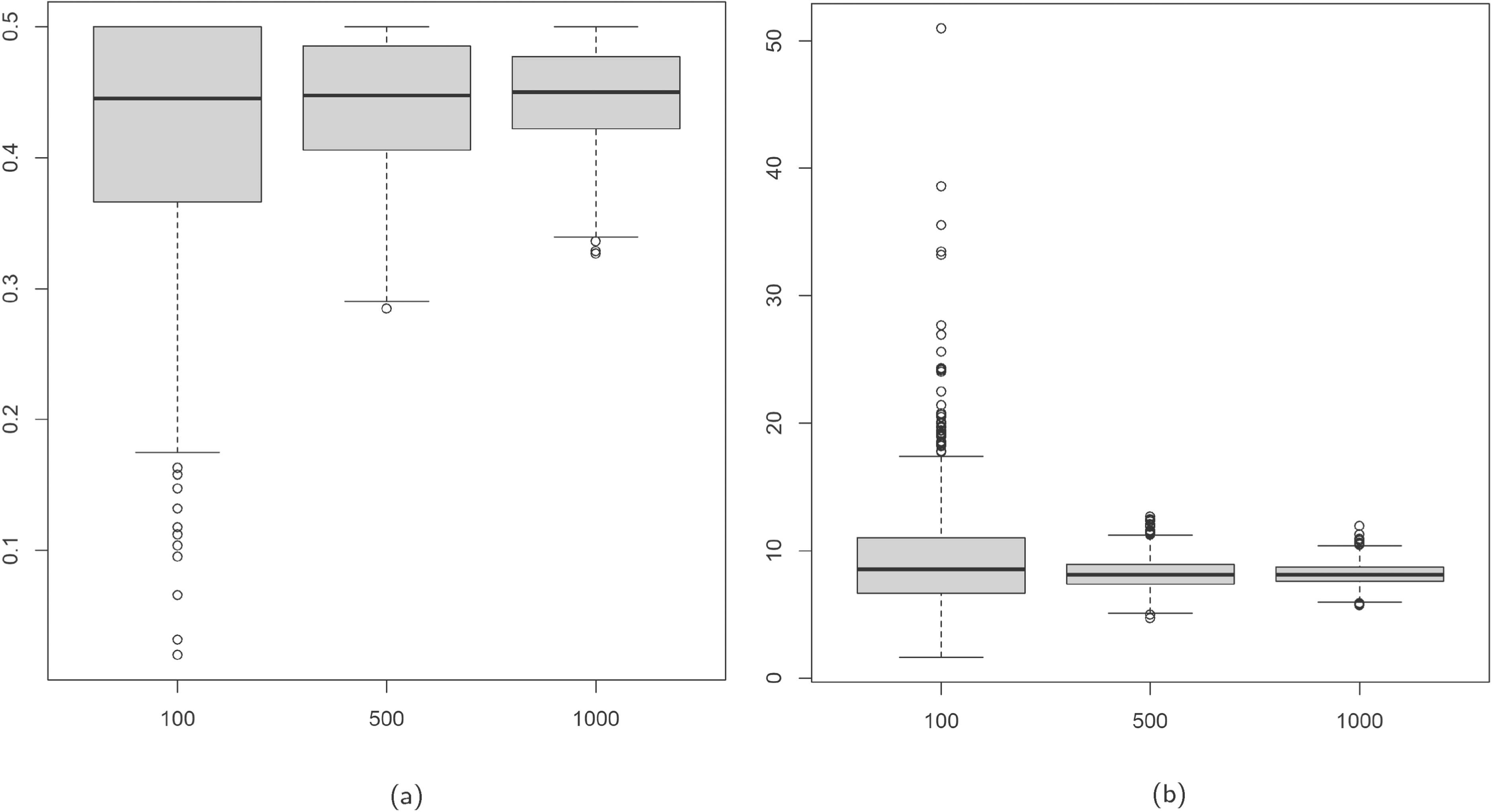
Boxplots of
In this study, we perform a sensitivity analysis to investigate the impact of a single atypical observation on the Poisson-RM, NB-RM, and cNB-RM. We generate datasets of size Close: A response value Far: A response value
An example of a dataset generated with the above schemes is given in Figure 9, where the outlier is added to the generated NB data and illustrated in green for the close case and red for the far case. For each configuration,
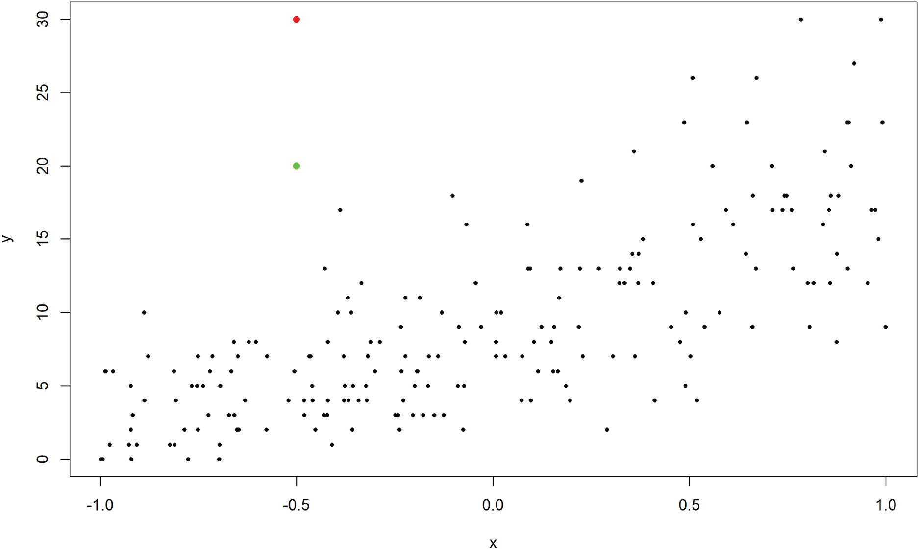
Example of simulated negative binomial (NB) data with the single outlier illustrated in red.
Simulation results of sensitivity analysis for added outlier based on
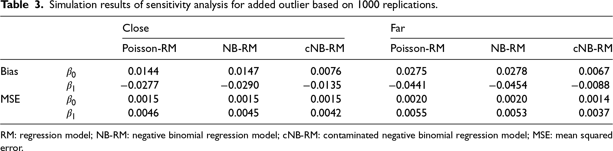
RM: regression model; NB-RM: negative binomial regression model; cNB-RM: contaminated negative binomial regression model; MSE: mean squared error.
We observed that the estimates of the regression coefficients of the Poisson-RM and NB-RM exhibit more bias compared to the cNB-RM. This is even more pronounced for the far case. Relatedly, the MSE is lower for the estimates of the regression coefficients of the cNB-RM than for the other two models.
To assess the ability of the cNB-RM to automatically classify whether a point is good or bad using (8), following the approach by Punzo and McNicholas, 17 we report: (i) the true positive rate (TPR), which measures the proportion of atypical observations that are correctly identified as atypical; and (ii) the false positive rate (FPR), which corresponds to the proportion of typical points incorrectly classified as atypical. The results are reported in Table 4.
Classification results of cNB-RM for close and far scenarios.
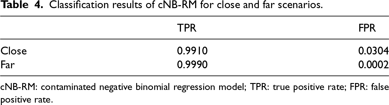
cNB-RM: contaminated negative binomial regression model; TPR: true positive rate; FPR: false positive rate.
For the close case, of the 1000 added atypical observations to the 1000 generated datasets, 991 were classified as atypical, leading to a TPR of 0.991. Similarly, of the
The cNB-RM is applied to real-world benchmark datasets, namely the
As mentioned in Section 1, if the observed zeros in the data exceed the distributional assumption of the model, this can also be a cause of overdispersion. Generally, when overdispersion arises as a result of an excess amount of zeros, a suitable strategy is to model the data using either a zero-inflated Poisson (ZIP, Lambert
37
) or a zero-inflated negative binomial (ZINB, Yau et al.
38
) model. The model performance is ranked as usual
28
via the Akaike information criterion (AIC; Akaike
39
) and the Bayesian information criterion (BIC; Schwarz
40
). Moreover, the likelihood-ratio (LR) test, which compares nested models, can be used to determine whether the cNB-RM (alternative model) significantly improves upon the NB-RM (null model) since the cNB-RM includes the NB-RM as a special case (see Proposition 1). Under the null hypothesis of no improvement, the test statistic is

In the first application, we refocus our attention on the
From Table 5, it is apparent that the cNB-RM outperformed all the considered models based on the AIC and BIC. This is further corroborated by the LR test (11) which has a
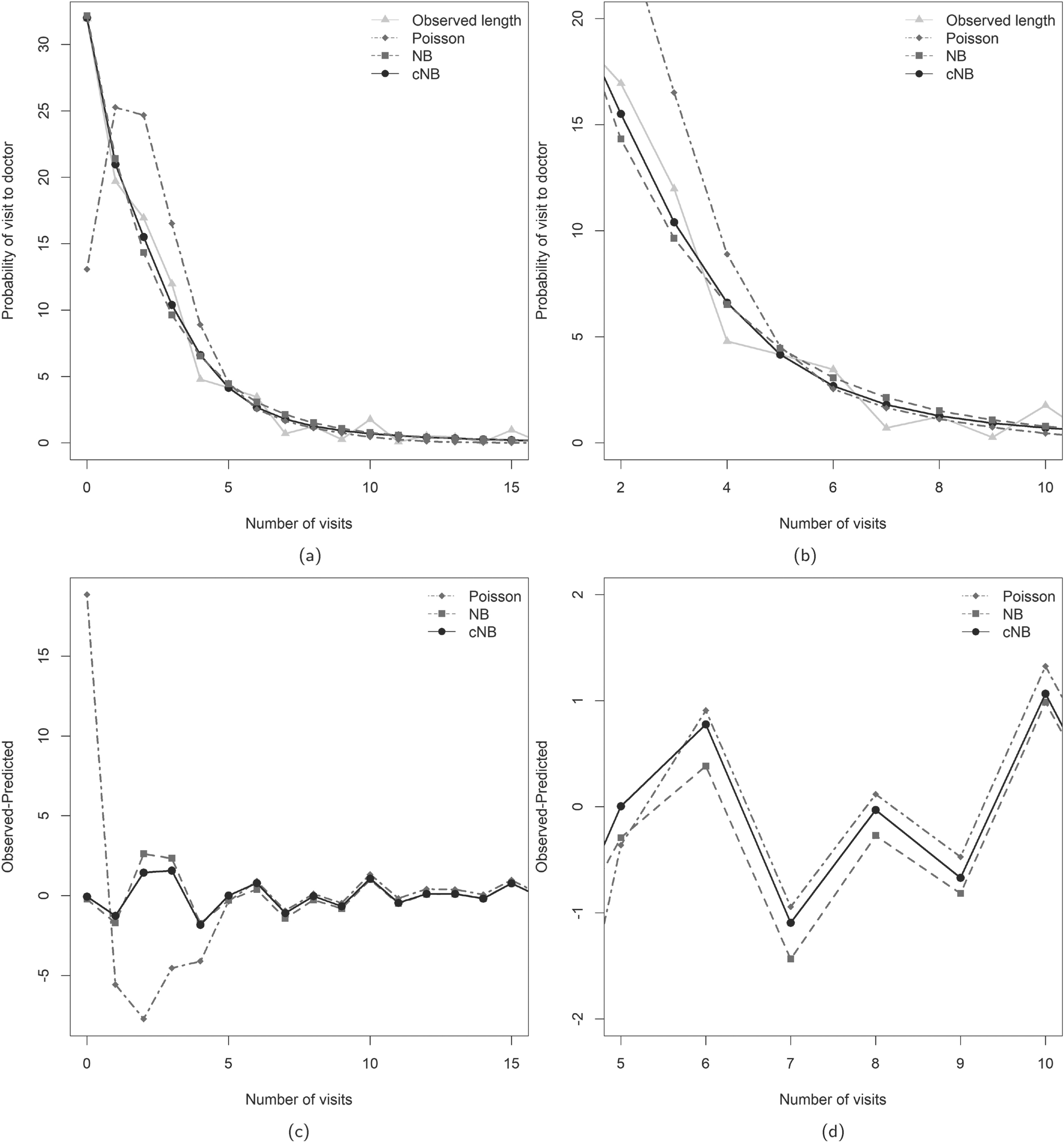
Observed proportions and predicted probabilities for the number of doctor visits: (a) observed proportions and predicted probabilities; (b) magnified observed proportions and predicted probabilities; (c) difference between observed proportions and predicted probabilities; (d) magnified difference between observed proportions and predicted probabilities.
Ranking of fitted regression models to
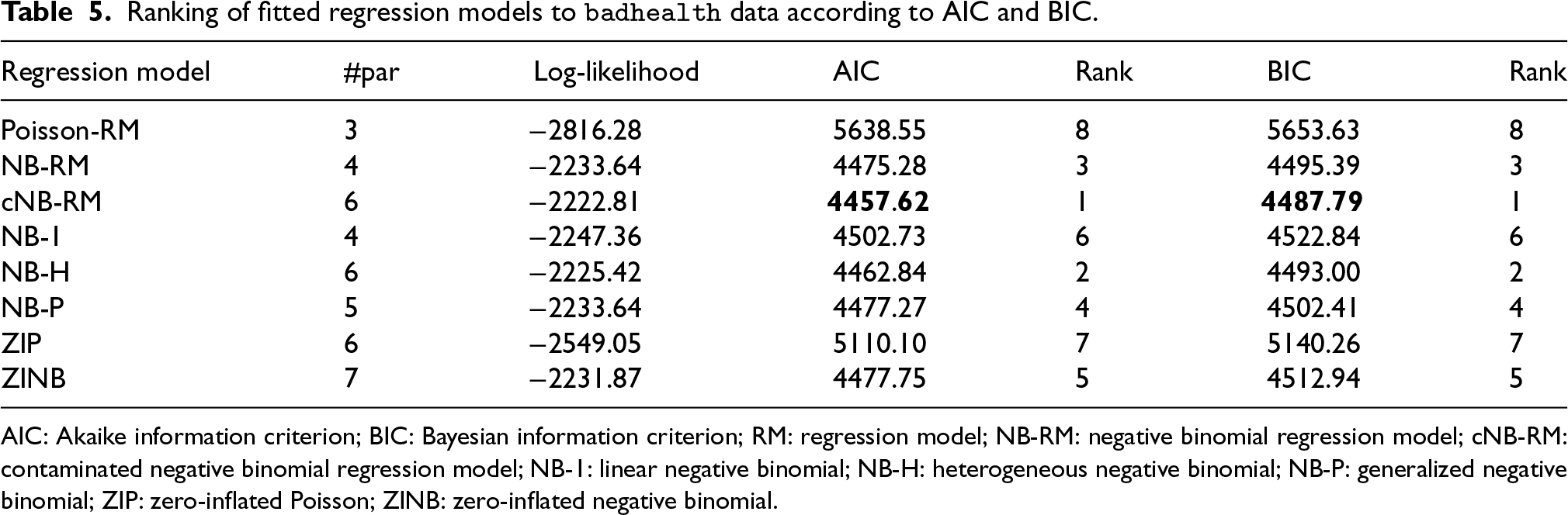
AIC: Akaike information criterion; BIC: Bayesian information criterion; RM: regression model; NB-RM: negative binomial regression model; cNB-RM: contaminated negative binomial regression model; NB-1: linear negative binomial; NB-H: heterogeneous negative binomial; NB-P: generalized negative binomial; ZIP: zero-inflated Poisson; ZINB: zero-inflated negative binomial.
Estimated coefficients and corresponding SEs (in brackets) of NB-RM and cNB-RM to
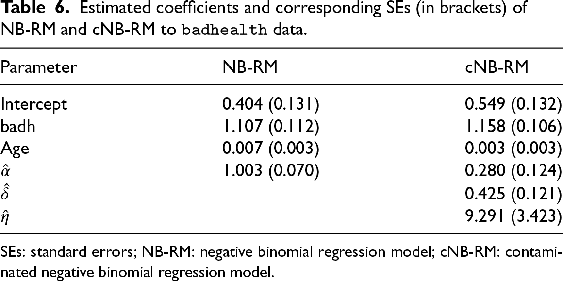
SEs: standard errors; NB-RM: negative binomial regression model; cNB-RM: contaminated negative binomial regression model.
The
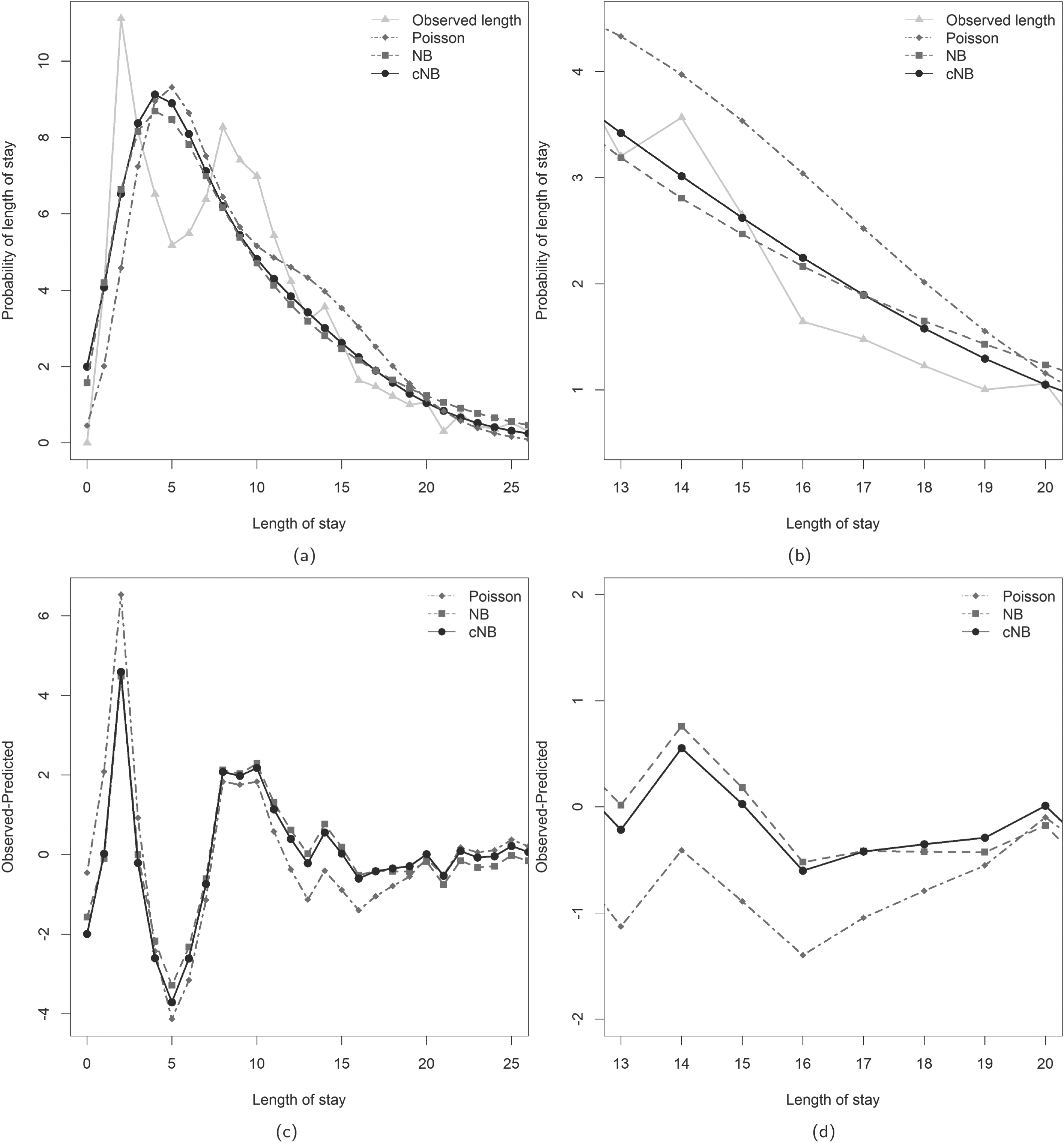
Observed proportions and predicted probabilities for the length of stay: (a) observed proportions and predicted probabilities; (b) magnified observed proportions and predicted probabilities; (c) difference between observed proportions and predicted probabilities; (d) magnified difference between observed proportions and predicted probabilities.
Ranking of fitted models to
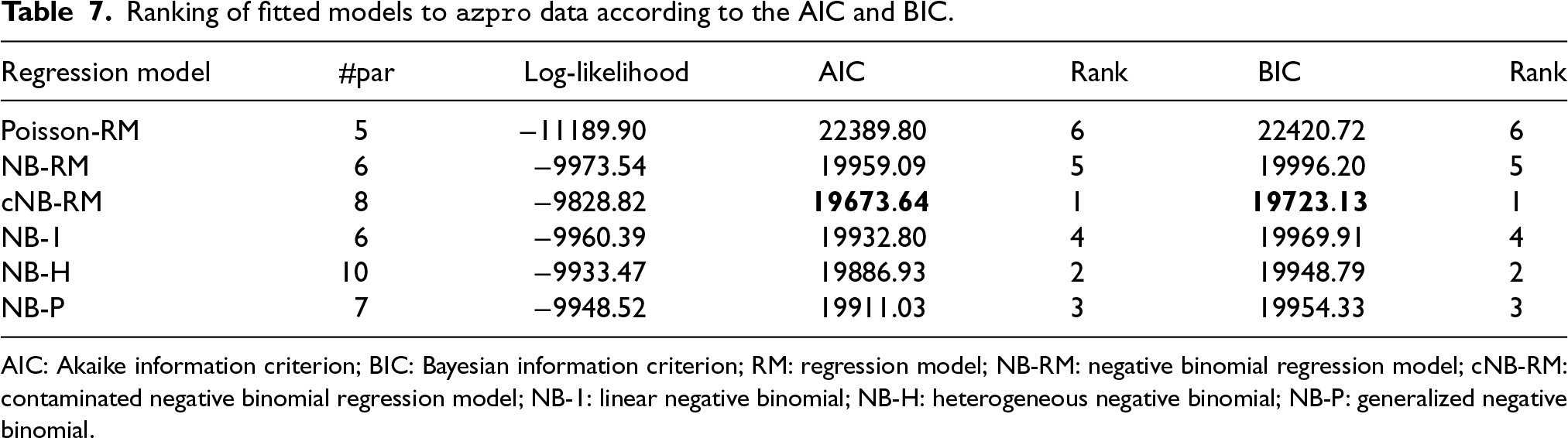
AIC: Akaike information criterion; BIC: Bayesian information criterion; RM: regression model; NB-RM: negative binomial regression model; cNB-RM: contaminated negative binomial regression model; NB-1: linear negative binomial; NB-H: heterogeneous negative binomial; NB-P: generalized negative binomial.
Estimated coefficients and corresponding SEs (in brackets) of NB and cNB regression models fitted to
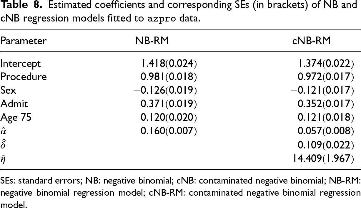
SEs: standard errors; NB: negative binomial; cNB: contaminated negative binomial; NB-RM: negative binomial regression model; cNB-RM: contaminated negative binomial regression model.
In this article, we introduced a straightforward extension of the NB-RM, termed contaminated NB-RM (cNB-RM). This model not only addresses overdispersion more effectively than the NB-RM but also offers greater flexibility in accommodating the conditional skewness and excess kurtosis observed in real (health) data. Relatedly, real-world data frequently includes mild outliers and extreme values, which significantly impact all the statistical moments largely discussed in this article, namely mean, variance, skewness, and kurtosis. Advantageously, our proposed model is formulated as a simple mixture of two NB-RMs with the same means but different dispersion parameters, and this formulation not only retains a closed-form expression for the probability mass function of the conditional response variable but also provides the capability, if desired, to identify mild outliers. These outliers can be understood as observations stemming from the contaminant NB-RM, distinct from the regular observations associated with the reference NB-RM. Last but not least, the simple formulation of our proposal involves two additional parameters having practical interpretation, an aspect of fundamental importance not only for statisticians but also for practitioners who use statistical models and want to interpret the output from the considered model. These parameters are the proportion of observations originating from the contaminant NB-RM (potentially considered as mild outliers or extreme values) and the degree of contamination. This degree of contamination roughly quantifies how dispersed the observations in the contaminant NB-RM are compared to those in the regular distribution.
Furthermore, an EM algorithm for ML estimation of the parameters of the cNB-RM is proposed. A parameter recovery study is performed to assess the EM algorithm’s accuracy in retrieving the true generating parameters. The impact of outliers on parameter estimation and their potential to introduce bias into the regression parameters, which could distort inferences and overestimate the overdispersion parameter of the NB-RM when it compensates for the outliers, are examined through a sensitivity analysis.
Regarding real-world scenarios, we utilized the cNB-RM on two benchmark health datasets and compared its performance with other NB variations, including a zero-inflated NB-RM. In both cases, the cNB-RM demonstrated superior performance over the considered regression models, highlighting its viability as an alternative model for overdispersed count data. While the proposed models are motivated by applications in health, their use is not restricted to this field and other fields may benefit from its use.
Future extensions of the cNB-RM could include allowing the contamination parameters
Footnotes
Acknowledgements
Ferreira and Bekker have been partially supported by (i) the National Research Foundation (NRF) of South Africa (SA), grant RA201125576565, nr 145681; RA171022270376, grant no: 119109; and (ii) the DSI-NRF Centre of Excellence in Mathematical and Statistical Sciences (CoE-MaSS)—grants 2024-033-STA and 2024-034-STA, South Africa. Bekker also acknowledges the support of the National Research Foundation (NRF) of South Africa (SA) ref. SRUG2204203865 nr. 120839. The opinions expressed and conclusions arrived at are those of the authors and are not necessarily to be attributed to the NRF.
Data availability
All datasets considered in this article are freely available in
Declaration of conflicting interests
The author(s) declared no potential conflicts of interest with respect to the research, authorship and/or publication of this article.
Funding
The author(s) disclosed receipt of the following financial support for the research, authorship, and/or publication of this article.
A. Proofs
Proof Proposition 1: The cNB-D in (4) has the hierarchical representation
if if if if