






Abstract
Methods of causal discovery aim to identify causal structures in a data-driven way. Existing algorithms are known to be unstable and sensitive to statistical errors, and are therefore rarely used with biomedical or epidemiological data. We investigate an algorithm that efficiently exploits temporal structure, so-called tiered background knowledge, for estimating causal structures. Tiered background knowledge is readily available from, for example, cohort or registry data. When used efficiently it renders the algorithm more robust to statistical errors and ultimately increases accuracy in finite samples. We describe the algorithm and illustrate how it proceeds. Moreover, we offer formal proofs as well as examples of desirable properties of the algorithm, which we demonstrate empirically in an extensive simulation study. To illustrate its usefulness in practice, we apply the algorithm to data from a children’s cohort study investigating the interplay of diet, physical activity and other lifestyle factors for health outcomes.
Introduction
Discovering causal structures in data is a challenging task. Ideally, we would like to input data into an algorithm that outputs one or more plausible causal directed acyclic graphs (DAGs) linking variables in data. Such data-driven approaches for estimating a causal DAG are known as causal discovery (or causal search, structure learning, etc.). While algorithms for causal discovery were first developed in the field of computer science more than 30 years ago 1 and have, since then, continually been generalised and refined, 2 their use with biomedical or epidemiological data is still rare (other than in genetics 3 ). Some exceptions are examples investigating the complex clinical performance of implants, 4 applications to epidemiologic cohort studies5,6 or the causal analysis of episodes of schizophrenia. 7
Causal analyses often aim at causal effect estimation. Such analyses typically assume the causal structure, that is, DAGs, to be given, usually derived from domain expertise, which may entail ‘confirmation bias’ among many other issues. Moreover, the question whether the expert knowledge is correct or compatible with the data is typically not addressed. 8 Data-driven methods for estimating causal DAGs provide an alternative, or supplement, to relying solely on expert knowledge. 9 For instance, in the context of building a life-course model for depression in early old age, it was found that different experts’ causal DAGs and the output of a causal discovery algorithm exhibited considerable disagreement. 10 But the comparison also suggested that the discovery algorithm detected several causal relations which were, post-hoc, found to be plausible by experts.
While promising and potentially useful, algorithms for causal discovery face a number of issues in practical applications (see recent overviews by Didelez 9 and Textor 11 ). One major problem is that they can be unstable or ambiguous with finite data due to sensitivity to sampling variation. Rigorous treatments of the finite-sample performance of causal discovery are rare. Some consideration is given to asymptotic properties,12,13 but most analyses of their properties focus exclusively on the ‘oracle’ case where infinite data or exact knowledge of the joint distribution is assumed. In this paper, we describe how temporal structure of the data, or more generally tiered background knowledge, can efficiently be exploited to improve causal discovery algorithms on finite samples, rendering the methods more stable and robust for practical applications. This is very useful as temporal information is often available in biomedical or epidemiological data, for example, when using patients’ records or cohort data as in life course epidemiology, 14 and it is usually unambiguous and correct.
We will focus on the Peter-Clark (PC) algorithm,1,15 which is a so-called constraint-based causal discovery algorithm. It has the advantage that it is flexible, allowing for various extensions and adaptations to different data types. However, the PC algorithm also suffers from two types of limitations: one is a lack of causal identifiability and the other is sensitivity to statistical errors. The first problem is due to the symmetric nature of conditional independence testing, which implies that some causal directions cannot be identified even from ‘infinite data’. Additional (non-independence) assumptions about, for example, the functional forms of the causal relations can help identify causal direction (see e.g. Hoyer et al. 16 or Tillman et al. 17 ). In contrast, the second problem occurs in practice when we apply the algorithm to finite samples, as mentioned above. While the PC algorithm has desirable asymptotic properties,12,13 with finite samples it is especially prone to errors due to erroneous conclusions based on statistical tests propagating through the many stages of the algorithm. It was previously shown that tiered background knowledge has the potential to improve the informativeness of the estimated graphs from infinite data. 18 In the present paper, we specifically address how to incorporate tiered background knowledge with finite samples. This is an interesting task because in the oracle case it does not matter at what stage of the algorithm tiered (or any correct) background knowledge is used, while in finite samples it must be used in a certain way to not create contradictions. Further, it can be used to reduce the number of statistical tests and hence to reduce opportunities for statistical errors. We investigate the resulting finite-sample properties and show how efficient use of tiered background knowledge increases the robustness towards statistical errors yielding more accurate outputs.
We consider an extension of the PC algorithm that exploits tiered background knowledge, and we refer to this as the tiered PC (tPC) algorithm. Such an extension was previously suggested,5,6,15,19 and versions of the tPC algorithm have been implemented in TETRAD software 20 and R packages,21–23 and have been applied.5,6 Previous work concerning tiered background knowledge has focused on theoretical properties in large sample cases. It has not yet been addressed how tiered background knowledge is used most efficiently, and to our knowledge, this paper is the first to thoroughly examine the finite-sample properties of the tPC algorithm. We here provide theoretical results, an extensive simulation study and a data application.
The outline of the paper is as follows. Section 2 introduces the basic concepts of the paper, which we illustrate with a toy example of a children’s cohort study. Section 2.2 describes versions of the PC algorithm, and Section 2.3 formally introduces the concept of (tiered) background knowledge. In Section 3, we introduce the basic tPC algorithm and a tiered version of the Lists-Majority rule-PC-stable (LMPC) algorithm 24 (the tiered algorithms), and show some important properties. In Section 4, we conduct an extensive simulation study exploring the finite-sample performance of the tLMPC-stable algorithm. In Section 5, we show how the algorithm can be used in practice by applying it to data from a children’s cohort study investigating the interplay of diet, physical activity and other lifestyle factors with regards to several health outcomes. 25 Finally, Section 6 provides a discussion of the results.
Basic concepts
In this section, we introduce the formal graphical framework and describe the existing algorithms. Detailed background can be found in Supplemental Appendix A.1. As (constraint-based) causal discovery reconstructs the causal structure from the pattern of conditional independencies in the data, we focus on the relations between graphs, causal relations and conditional (in)dependencies.
Graphs
A graph
Graphical models link graphs and probability distributions, and we let the nodes represent random variables: with
We are interested in causal relations underlying the data, and we therefore focus on DAGs, which only contain directed edges and have no directed cycles. A directed edge
In order to represent causal structures using DAGs, we need to make the assumption of causal sufficiency: for each pair of nodes (variables), all their common causes are nodes in a DAG.
(G raph terminology and interpretation)
In the DAG Toy example of a graph representing the variables in a cohort study. (a) A DAG 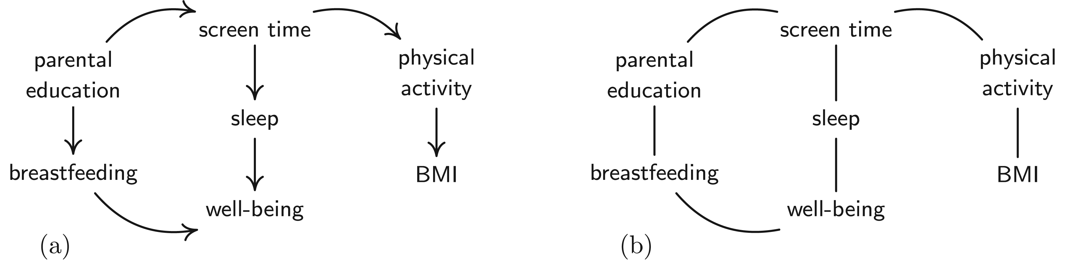
Since the node Examples of DAGs: (a) a subgraph of 
As we have seen in the example of Figure 2, different DAGs can induce the same set of d-separations and we then refer to them as Markov equivalent. We refer to a class of Markov equivalent graphs as a (Markov) equivalence class. An equivalence class of DAGs is represented by a CPDAG (a full characterisation of CPDAGs can be found in Andersson et al.
26
). A CPDAG is partially directed in the sense that it contains both directed and undirected edges: the undirected edges represent edges that are directed in one direction in some DAGs in the equivalence class, and in the opposite direction in other DAGs, while the directed edges represent edges that are common to all DAGs in the class. If a CPDAG represents a class of causal DAGs, we will refer to it as a causal CPDAG, and in a causal CPDAG, we will interpret undirected edges
Assuming the Markov properties, graphs encode conditional independencies among a given set of variables. Constraint-based causal discovery aims to solve the inverse problem: to estimate a graph from the conditional independencies in a given dataset by performing a series of statistical tests for conditional independence. Other types of causal discovery methods operate under different assumptions and use different strategies such as, for example, optimising a score function (see e.g. Chickering 28 ), but these will not be discussed here.
When estimating graphs based on conditional independence tests, a key assumption is the reverse of the global Markov property: a distribution is faithful to a graph if any conditional independence in the distribution corresponds to d-separation encoded by the graph (see Definitions 7 and 9 in Supplemental Appendix A.1). Even under faithfulness, and given the correct independence model, we are still limited by the fact that multiple DAGs can be Markov equivalent.
The basic PC algorithm 15 is a constraint-based algorithm that estimates a CPDAG. The main steps are as follows.
The basic PC algorithm
Start with a complete undirected graph over the given nodes. Visiting every pair If Orient further edges according to Meek’s rules 1–3
27
(see Figure 11 in Supplemental Appendix A.2) until none of the rules apply anymore.
The basic PC algorithm makes use of faithfulness in phase (II) to construct the skeleton, and of the particular conditional independencies encoded by v-structures in phase (III).
When analysing the properties of causal discovery methods, the oracle version and the sample version should be distinguished. The oracle version refers to the algorithm when the input are the true conditional independencies. Under faithfulness and causal sufficiency, the oracle version of the basic PC algorithm is sound 15 and complete, 27 that is, the correct and most informative CPDAG is obtained. The sample version refers to the case where the input consists of conditional independencies found by statistical tests on finite data. These tests make statistical errors so that the input is not necessarily correct. Crucially, early errors can propagate through all iterations of the algorithm because deleted edges cannot be reinstated and updated adjacencies are used in each round of the skeleton phase (II). The sample version of the basic PC algorithm therefore does not typically output the correct CPDAG, it may not even output a valid CPDAG, in the sense that it does not represent an equivalence class of DAGs.
Moreover, the output of the sample version of the basic PC algorithm depends on the sequence (order) in which the variables are visited. To account for this, a modification has been introduced, the so-called LMPC-stable algorithm, 24 which is order independent through three phase specific modifications to (II–IV). We provide a short summary of the modifications and refer to the literature for details. 24
The LMPC-stable algorithm
At the beginning of each round, for each node Majority rule: determine whether each Orient remaining undirected edges with Meek’s rules only if they are not ambiguous. If conflicts occur, indicate these using bidirected edges.
Like the basic PC, the oracle version of LMPC-stable is sound and complete, but its sample version has better properties, for example, it is order independent and it can be expected to propagate fewer errors. An alternative modification is the conservative PC (CPC) algorithm,
29
where phase (III) requires
Conflicting edges and ambiguous triples make the estimated graph difficult to interpret since it no longer necessarily represents an equivalence class. However, they reflect the uncertainty entailed by finite data.
Often external background knowledge on some aspects of the true causal structure is available. Such background knowledge implies that graphs have more in common than just the independence model. In this section, we show how incorporating background knowledge can improve the informativeness, that is, help us orient otherwise undecidable edges. In Sections 3 and 4, we show how background knowledge can reduce errors and conflicts.
We define background knowledge as a pair
In this paper, we are concerned with tiered background knowledge as given, say, by a partial temporal ordering of the variables, for example, due to a cohort study design:
(Tiered ordering)
Let
If there are multiple orderings,
A tiered ordering entails background knowledge in the following way:
(Tiered background knowledge)
Let
In previous work, it was shown how tiered background knowledge can be combined with a consistent CPDAG yielding a restricted equivalence class represented by a tiered MPDAG with desirable properties. 18 Example 2 illustrates how tiered background knowledge improves the informativeness by orienting all cross-tier edges.
(Cross-tier edge)
Let
The DAG
The following more complex example shows that more than just the cross-tier edges are oriented as a consequence of tiered background knowledge.
Consider the nodes in DAG
The corresponding CPDAG and tiered MPDAG are given in Figure 3. With tiered background knowledge two cross-tier edges are oriented, and with Meek’s rules two more edges can be oriented. In total, six out of seven edges are directed in the tiered MPDAG, while only two of seven are directed in the CPDAG which uses no background information.
Toy example of a children’s cohort study. Left: CPDAG. The edges are oriented because they form a v-structure, in this particular graph no orientations follow from Meek’s orientation rules. Right: Tiered MPDAG. Edges are oriented either because they are part of a v-structure, they are cross-tier edges, or they follow from Meek’s orientation rules.
A first approach for combining background knowledge with a discovery algorithm is to impose it post-hoc onto the output; we call this the naive tiered PC (naive tPC) algorithm. In particular, this means that the background knowledge is not exploited to estimate the equivalence class itself. In the next section, we address how to improve upon the naive approach which we first define here as follows:
The naive tPC algorithm
Estimate a CPDAG For each adjacent pair of nodes In addition to Meek’s rules 1–3, Meek’s fourth rule is applied to
The oracle version of the naive tPC algorithm is sound and complete (this follows directly from Meek’s work 27 ). However, the sample version of the naive tPC algorithm has a major flaw: the estimated CPDAG of step 1 is not guaranteed to be consistent with the tiered background knowledge. While we can impose inconsistent background knowledge by over-ruling the estimated graph as in step 2, where edge directions may be reversed, it appears more sensible to ensure consistency throughout the algorithm. Moreover, if the background knowledge is correct, exploiting it early on should reduce statistical errors and decrease the required conditional independence tests, as the next Example 4 illustrates.
Assume that we are given three nodes
Tiered background knowledge can also be used to estimate the equivalence class itself which the naive tPC does not exploit. In the next section, we contrast the naive approach with a more efficient approach that uses the tiers early on, before orienting the cross-tier edges.
We now introduce a way how to ensure consistency with the tiered background knowledge throughout the sample versions of the search algorithms while avoiding any unnecessary conditional independence tests. Below we describe how the phases of either the basic PC or the LMPC-stable algorithm are to be altered. We loosely refer to this as ‘the tPC algorithm’ or ‘the tiered algorithms’; when specifically applied to the basic PC algorithm we obtain the ‘basic tPC’ algorithm and when applied to the LMPC-stable algorithm we obtain the ‘tLPMC-stable’ algorithm. Due to its better finite-sample properties, we mostly focus on the tLMPC-stable algorithm of which formal details are provided as Algorithm 1 in Supplemental Appendix B.
The basic tPC/tLMPC-stable algorithm
Apply the following modifications to either the PC or the LMPC-stable algorithms: Only test whether A pattern Additional orientation of cross-tier edges: Any undirected edge In addition to Meek’s rules 1–3, Meek’s 4th rule is applied as well.
The modifications of (II) and (III) reflect that variables in the future cannot be direct causes of earlier ones, and are thus not needed for obtaining independence. The modification of (IIIa) takes into account that if
The following result establishes soundness and completeness of the oracle version of the basic tPC and tLMPC-stable algorithms. Versions of constraint-based algorithms using tiered background knowledge have been considered by others, and the correctness must have been assumed by the authors. However, we are not aware of a formal proof in the literature, and we state and show this for the sake of completeness.
Let
The proof of Proposition 1 can be found in Supplemental Appendix E for the tLMPC-stable algorithm (Algorithm 1). A similar argument holds for the basic tPC.
This result means that the oracle versions of the tiered algorithms output the unique MPDAG representing the independence model and the tiered background knowledge, that is, separating sets ‘in the future’ can indeed be ignored as in phases (II) and (IIIa). However, the oracle version of the naive tPC algorithm is also sound and complete, and we now turn to the properties under finite samples. We have the following proposition.
Let
Unlike the sample version of the naive tPC algorithm, the sample versions of the basic tPC or tLPMC-stable algorithm are therefore guaranteed to be consistent with the tiered background knowledge before using it to orient the cross-tier edges.
Proposition 2 only concerns the skeleton and the v-structures. In phase (IIIb), background knowledge adds more information to the estimated graph, and potentially creates more v-structures. Note that it is important to apply Meek’s rules only in phase (IV) after (IIIb). If we were to switch (IIIb) and (IV) of the tiered algorithms, the sample version would not guarantee the consistency with the tiered background knowledge of all orientations following the application of Meek’s rules. Hence, we should orient cross-tier edges before applying Meek’s rules in order to avoid unnecessary errors, as illustrated in the following example.
Consider the DAG Example of how tiered background knowledge can prevent statistical errors. (a) The true DAG 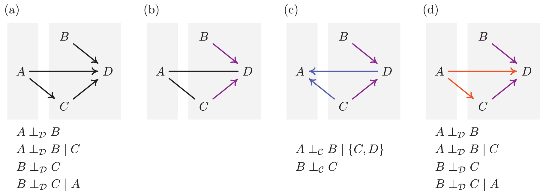
Suppose now that we switch phases (IIIb) and (IV). Then, under the above erroneous independence, we would obtain the graph in Figure 4(b) after the v-structure phase (IIIa), and the graph in Figure 4(c) after applying (IV) Meek’s rules. Clearly, the two new edge orientations violate the tiered ordering, and in addition, the graph does not encode the correct independencies. Since early errors in the algorithm might propagate through the following steps, in particular through Meek’s rules, as illustrated here, it is important to exploit background knowledge as early as possible and only apply Meek’s rules at the end.
Returning to the tiered algorithms as proposed here, phase (IIIb) would orient cross-tier edges and obtain the graph in Figure 4(d). This graph is consistent with the tiered background knowledge, and we have in fact recovered the full DAG. Note that even though phase (IIIa) could not recover the v-structure
As mentioned in Section 2.2, statistical errors may result in the output of the sample version of the basic PC algorithm being dependent on the order in which the independence tests are performed, and thus on the input sequence of the variables. This order dependence is eliminated by the LMPC-stable algorithm. Here, we establish formally that the tLMPC-stable algorithm is also order independent.
The output of the tLMPC-stable algorithm does not depend on the sequence in which the variables are visited.
The proof of Proposition 3 can be found in Supplemental Appendix E.
As discussed in Section 2.2, the output of the sample version of the LMPC-stable algorithm may contain bidirected edges, and the same is the case for the tLMPC-stable algorithm. However, the latter can be expected to have fewer bidirected edges since some of the conflicts might be prevented or resolved by the tiered background knowledge. We illustrate this empirically in Section 4. This means that even in cases where LMPC-stable algorithm does not output a valid CPDAG, it might still be possible to obtain a valid tiered MPDAG with the tLMPC-stable algorithm.
In the remainder, we only consider the LMPC- or tLMPC-stable algorithms when we refer to the (t)PC algorithms.
In the oracle version of the PC algorithm the benefit of incorporating (tiered) background knowledge is that we cannot lose, and typically gain, informativeness by possibly orienting some of the undirected edges. However, the same is not valid for the sample version: the restricted equivalence class output by the tiered algorithms can actually be larger than the output of the PC algorithm due to errors when using finite samples. Hence, there might not be a gain in informativeness. An example is given in Supplemental Appendix B.1 illustrating how incorporating tiered background knowledge in the PC algorithm can increase the estimated equivalence class with finite samples. Instead, using tiered background knowledge offers robustness by reducing errors, as explained earlier, and in this way, we expect the output to be at least as or more reliable than the output obtained without background knowledge.
Regarding the infinite sample limit, the PC algorithm is statistically consistent for high-dimensional settings in the sense that the estimated CPDAG converges in probability to the true CPDAG under some regularity conditions. 12 The authors assume Gaussian data, and allow for the number of nodes to grow as a function of the sample size under the assumption of a particular type of sparseness. Using slightly different assumptions, statistical consistency can be shown for a broader distributional class with Gaussian copula. 13 The statistical consistency results directly extend to the LMPC-stable algorithm, 24 and it is straightforward to argue that the tiered algorithms inherit the statistical consistency property as well. In order to prove consistency, the crucial phases of the algorithm are the estimation of the skeleton and of the v-structures. The rest follows from the tiered ordering and Meek’s rules, and only depends on the quality of skeleton and v-structure estimation. Statistical consistency is shown by bounding the error rates from independence testing, which follows from the consistency of the estimated partial correlations. Since the tiered algorithms can be expected to decrease the number of tests carried out, the number of errors will obviously still be bounded, and one can use assumptions similar to those by Kalisch and Bühlmann 12 under which the tiered algorithms will be statistically consistent.
Simulation study
In this section, we conduct a simulation study to demonstrate how tiered background knowledge improves graph estimation. We use the precision and recall for specific characteristics of the estimated graphs and compare them in a variety of settings. First, we evaluate the estimation of the equivalence classes by considering adjacencies and v-structures of the estimated graphs. Second, we focus on the recovery of the causal information by considering ancestral relations in the graphs. Lastly, we compute the proportion of bidirected edges, and by this we demonstrate the reduction of conflicts.
We compare different levels of tiered background knowledge: none, partial, detailed and full. These correspond, respectively to: running the regular LMPC-stable algorithm, the tLMPC-stable with a coarse ordering, a finer ordering and the full causal ordering of the variables. In addition, we compare the tLMPC-stable algorithm to the naive tPC algorithm of Section 2.3. As explained earlier, the latter does not use background knowledge to construct the equivalence class, it only imposes the background knowledge in a final step by orienting undirected and ambiguous edges according to the tiered ordering, as well as reversing any directed edges that are contradicting the background knowledge. By comparing the tLMPC-stable algorithm to the naive tPC algorithm (using LMPC-stable in the first phase), we demonstrate the importance of incorporating background knowledge as early as possible in the causal discovery algorithm.
Setup
The simulation study is performed using
For each simulated DAG, we partition the variables into five tiers. This means that for larger graphs, the tiers are larger, while for smaller graphs, knowing the full ordering will provide information on a large proportion of the edges. No background knowledge corresponds to a
Results
In this section, we include of the results of the main analysis obtained for graphs with 20 nodes. The remaining results can be found in Figures 14 to 22 in Supplemental Appendix C.3. The results of the analysis of the naive tPC algorithm are included in Figures 23 to 29 in Supplemental Appendix C.4. In addition to these two analyses, we explored the total number of tests and estimated edges, and the number of tests performed in each round (see Figures 30 to 33 in Supplemental Appendix C.5).
Figure 5 shows the median precision and recall of the estimation of the skeleton, that is, it assesses the quality of the detected presence/absence of edges. The recall clearly always improves when more detailed background knowledge is included. Thus, leveraging tiered background knowledge enables us to recover more correct adjacencies. Similar results can be found for other settings (see Figure 14 in Supplemental Appendix C.3). The improved recall comes at no or little loss in precision, as long as the chosen alpha value is not too high given the true sparsity level. This implies that with tiered background knowledge, the same or a slightly higher proportion of identified adjacencies are incorrect. For an instance with 100 observations, sparse graphs and an alpha value of 0.1 we find the precision goes from slightly above 90% without tiers to slightly below 85% with full tiered knowledge. A similar pattern is found for other settings in Figure 15 in Supplemental Appendix C.3. This can be explained by the tLMPC-stable algorithm performing fewer, and consequently different, independence tests when using more detailed background knowledge (see Figure 31 in Supplemental Appendix C.5), which tends to retain more edges (see Figure 30 in Supplemental Appendix C.5). It is remarkable that the recall of adjacencies improves at little cost in precision when using the tiered ordering because it does not even make use of orienting cross-tier edges, it only exploits that we do not need to consider separating sets in the future.
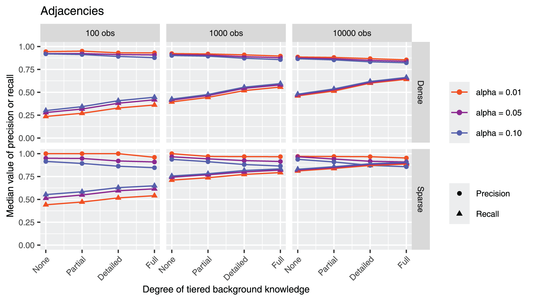
Median precision and recall of adjacencies from 1000 simulations in dense/sparse settings with 20 nodes and
In Figure 6 we find that including more background knowledge clearly improves the recall of v-structures. For dense graphs, including background knowledge also improves the precision, but for sparse graphs and large alpha we find a slight tendency to a lower precision. Similar results are found in Figures 16 and 17 in Supplemental Appendix C.3. It should be noted that the estimation of v-structures requires a locally correct estimation of the skeleton. This means that, for example, an improved recall of adjacencies improves the chance that the recall of v-structures will improve. Likewise, if the precision of adjacencies slightly decreases, then it is less likely that the precision of v-structures will increase. However, the plots in Figure 6 suggest an improvement for v-structures over and above what can be explained by the precision and recall of adjacencies. Moreover, the fact that we do not count v-structures consisting of one or two conflicting edges partly explains the low overall values of precision and recall.
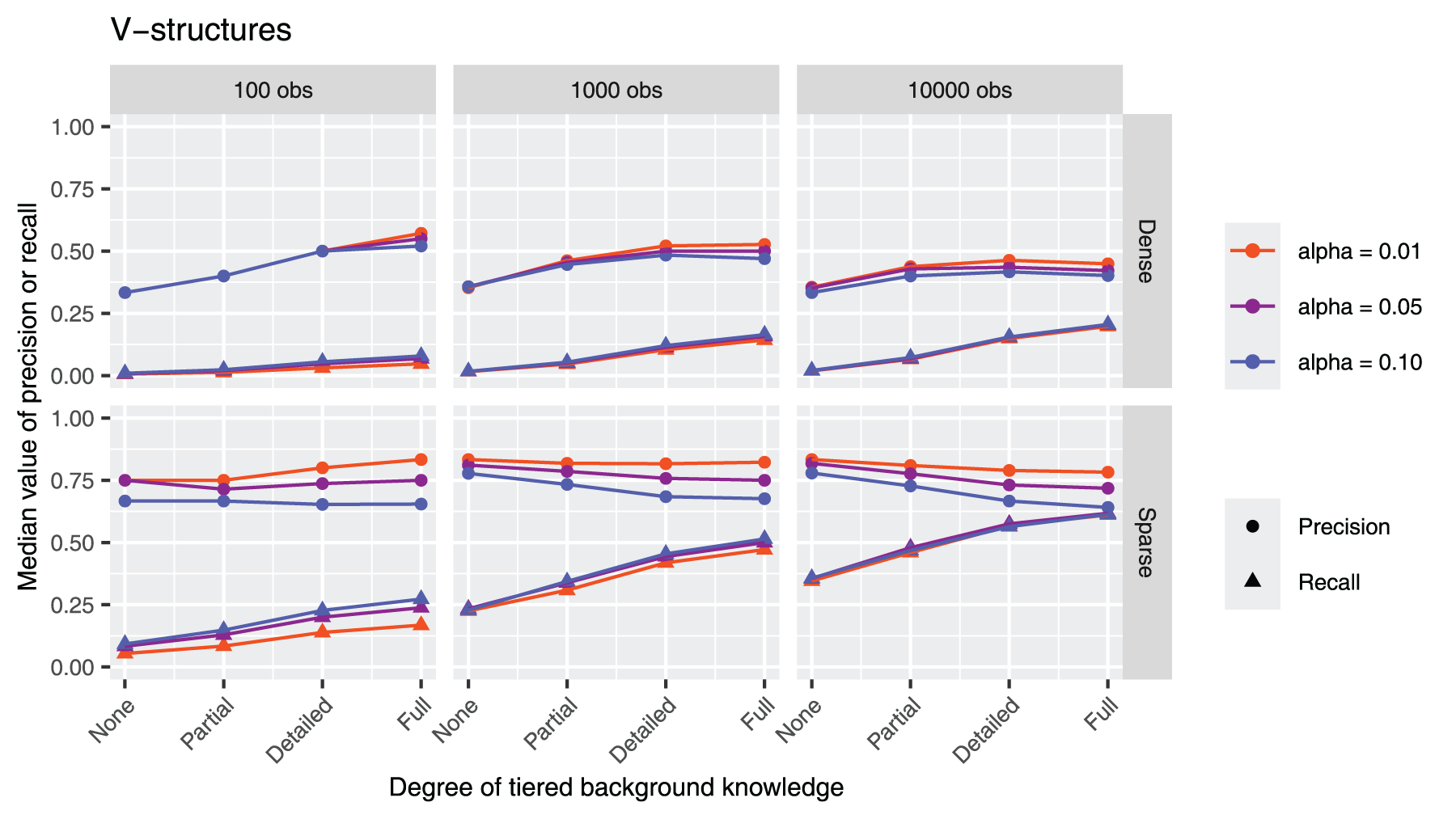
Median precision and recall of v-structures from 1000 simulations in dense/sparse settings with 20 nodes and
Figure 7 depicts the median precision and recall of the estimated ancestral relations (including parent–child relations), that is, this reflects the correctness of the directed paths and thus of (indirect) causal relations among the 20 nodes. Unsurprisingly, both clearly improve as the orientation of cross-tier edges using tiered background knowledge is guaranteed to be correct. With the tiered ordering we are thus able to recover more correct directed paths, which increases recall. At the same time, we disallow paths in the opposite direction, which limits the proportion of incorrect directed paths, increasing the precision. For sparse graphs and high alpha values, we find a minor decrease in precision, which is unsurprising given the lower precision of the skeleton (Figure 5). Similar results are found for all other settings (see Figures 18 and 19 in Supplemental Appendix C.3).
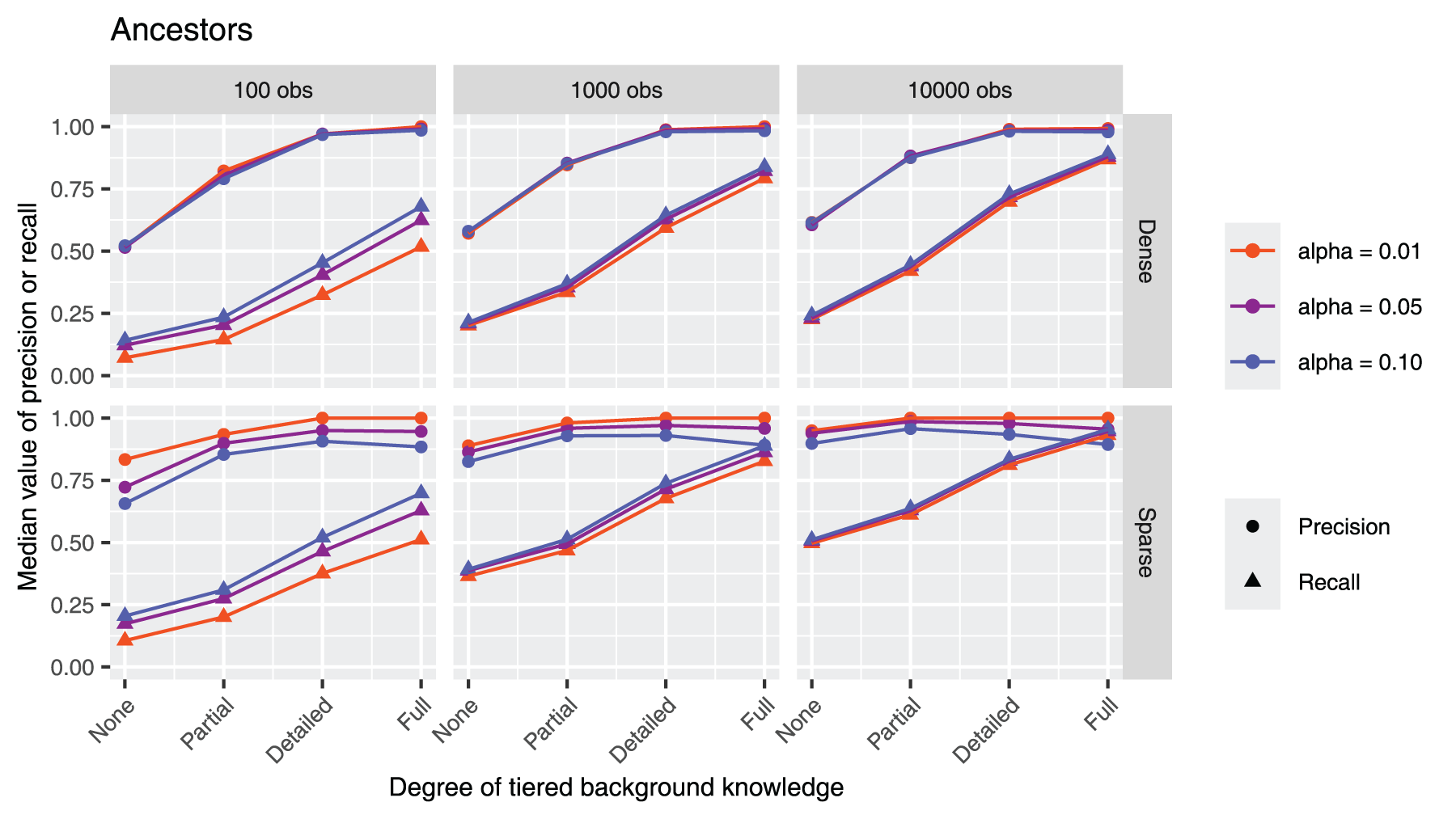
Median precision and recall of ancestors from 1000 simulations in dense/sparse settings with 20 nodes and
The median recall and precision of the estimated possible ancestral relations (i.e. partially directed paths among the nodes) are shown in Figure 8. Note that the true possible ancestors are determined from the respective true MPDAGs which are different depending on the detail of the tiers; this is in contrast to the skeleton, v-structures and ancestors of Figures 5 to 7, where the true proportions were based on the true DAGs. Hence, we see different patterns here: precision is very low for none or partial background knowledge but reaches 80% to over 90% for detailed and full tiers. Also for the recall, it has to be taken into account that the proportion of true possible ancestors can be dramatically smaller under full compared to no tiered background knowledge. Nevertheless, recall tends to slightly improve, except for a small decrease in dense graphs with larger sample sizes. It should be noted that possible ancestral relations is a much weaker property than ancestral relations, and graphs with very few directed edges can have many possible ancestral relations. Orienting edges may let us determine that a relation is ancestral and not just possibly ancestral, but orienting edges does not provide new possible ancestors. On the other hand, orienting edges may rule out some ancestral relations, which is why we find an increased precision.
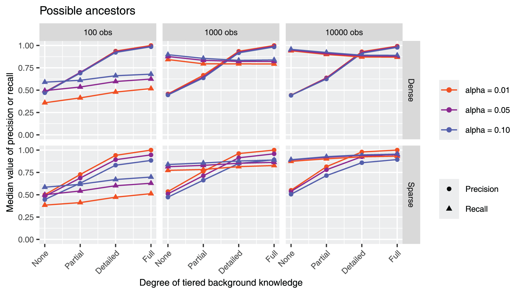
Median precision and recall of possible ancestors from 1000 simulations in dense/sparse settings with 20 nodes and
Importantly, Figure 9 (and Figure 22 in Supplemental Appendix C.3) depict the proportions of conflicting (bidirected) edges. These decrease as more background knowledge is included for all settings. Incorporating background knowledge enables the recovery of more true v-structures (Figure 16 in Supplemental Appendix C.3) and the orientation of cross-tier edges, correctly resolving conflicting information in the data.
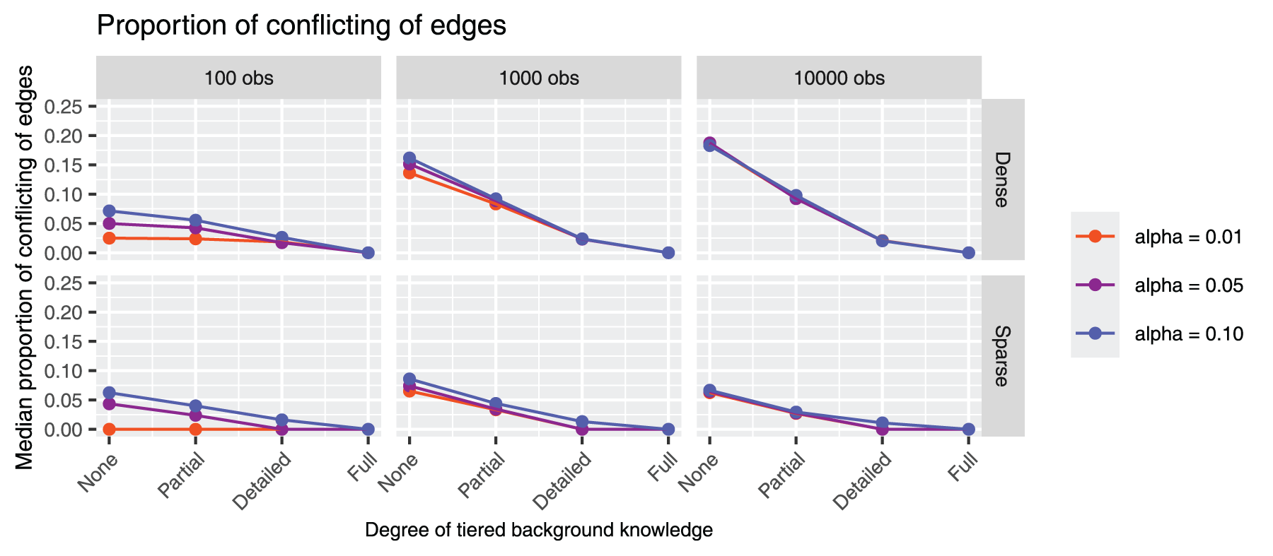
Median proportions of bidirected edges from 1000 simulations in dense/sparse settings with 20 nodes and
For the naive tPC algorithm (Figures 23 to 29 in Supplemental Appendix C.4), we see similar trends for the recovery of v-structures and ancestral relations as for the tLMPC-stable algorithm. However, the gains are much less pronounced than for the tLMPC-stable algorithm. Importantly, regarding the recovery of the skeleton, the naive tPC necessarily (using LMPC-stable in the first phase) gives the same result as the tLMPC-stable algorithm with no background knowledge (Figure 5) since the naive tPC algorithm does not make use of the background knowledge for estimating the skeleton.
As an example of how the tLMPC-stable algorithm performs in practice, we use it for estimating the causal structure of a subset of the data from the IDEFICS/I.Family study, 25 which is a prospective cohort study set up to explore the aetiology of nutrition related diseases among a cohort of children followed from early life through adolescence. The variables are measured in three waves several years apart, and this provides an initial, unambiguous tiered ordering of the variables. Moreover, the variables within the first tier can be subdivided into five tiers using expert knowledge: ‘context’, ‘early life 1’, ‘early life 2’, ‘early life 3’ and ‘baseline’. Note that while so-called context variables sometimes are assumed to have a special relation among them and to the remaining variables (e.g. Mooij et al. 32 ), we simply consider ‘context’ a regular tier set before everything else.
We will consider three tiered orderings, denoted by
Methods
We use the dataset provided by Foraita et al.,
6
where we select one of their 10 imputations of missing values for our analysis. The original aim was to answer specific research questions concerning the aetiology of body mass index (BMI). Here, our focus is on evaluating the algorithm’s performance. In particular, we aim to illustrate the benefits of incorporating tiered background knowledge and how different levels of detail improve the accuracy of graph estimation. For this reason, we restrict our analysis to data from Germany (
Results
The characteristics of the three estimated graphs are summarised in Table 1. All graphs have approximately the same density and share most of their adjacencies. In addition, the graphs with background knowledge (
Individual and shared characteristics of the graphs using
(no background knowledge),
(partial background knowledge) and
(detailed background knowledge).

Individual and shared characteristics of the graphs using
The estimated graphs can be found in Figure 10, and in Figures 34 and 35 in Supplemental Appendix D.2, and their respective adjacency matrices can be found in Figures 36 to 38 in Supplemental Appendix D.3. The estimated graphs of Figure 10 (detailed background knowledge) and Figure 35 in Supplemental Appendix D.2 (partial background knowledge) share almost all of the edge directions, and most of the directed edges are between repeated measurements. With partial background knowledge, all undirected edges are in the first tier. Some of these edges could be oriented using detailed background knowledge which illustrates the usefulness of imposing a finer ordering especially in the earliest tiers. 18

Estimated graph of the IDEFICS/I.Family dataset using the tLMPC-stable algorithm with detailed background knowledge (
The results demonstrate that the standard LMPC-stable (not using tiers) outputs numerous incorrectly directed edges. In Figure 34 in Supplemental Appendix D.2 these are indicated as dotted edges, where, for example, BMI of the child at baseline ‘causes’ birth weight (this erroneous direction is also present with partial tiers). Notably, the edges between repeated measurements are often directed against time without tiered ordering. None of this can occur in the output of the tLMPC-stable algorithm with the detailed tiers. In fact, many of the relations between repeated measurements are more plausible and compatible with subject matter, for example, the suggested feed-back relation between insulin resistance and BMI. Further, as the tLMPC-stable does not condition on the future, the correlation between some of the context variables (migrant, income, ISCED (International Standard Classification of Education)) is retained (undirected edges) which is more plausible than their (conditional) independence given future nodes as found in the absence of tiers. Moreover, the tLMPC-stable output contains some plausible directed edges not found without tiers, for example, from sex to BMI or from age to media. Finally, note that edge directions within tiers may be reversed as a consequence of orienting cross-tier edges; for instance, whether physical activity causes well-being or the other way around could be debated and there is disagreement between the different graphs, but when exploiting the tiers the direction suggests that physical activity affects well-being. However, even the output of the tLMPC-stable algorithm with detailed tiers contains some implausible structures and we caution against over interpreting a single output without measure of uncertainty, for example, by bootstrapping which was done in Foraita et al., 6 c.f. the next section.
It should be noted that neither of the estimated graphs in Figure 10 and Figures 35 and 34 in Supplemental Appendix D.2 are CPDAGs or MPDAGs. This happens because of the way the algorithm deals with conflicting or ambiguous information in the data. For example, in Figure 10 the undirected edge
Here we provide some further examples on how (constraint-based) causal discovery with tiered background knowledge has questioned current causal hypotheses and suggested alternatives in practical applications.
A detailed causal discovery analysis of the IDEFICS/I.Family using the tLMPC-stable algorithm with the full dataset of all participating countries, a larger set of variables, multiple imputation of missing values, uncertainty assessment using bootstrap and numerous sensitivity analyses can be found in Foraita et al. 6 Their discussion focused on BMI at wave 2 as a key outcome and revealed two interesting results. First, it was found that modifiable behaviours in early childhood, such as media time or physical activity, never (across bootstrap replications) had a direct effect on BMI in later childhood, but they always had an indirect effect. This is an interesting point and demonstrates the advantage of causal discovery over traditional multi-variable regression analysis (or similar): the latter would not be able to reveal such causal structures because in a regression, at best, only the direct causes of an outcome can be assessed. Indirect effects are also typically weaker which is compatible with findings of Börnhorst et al. 35 that even joint interventions on multiple modifiable behaviours reduced the risk of obesity in children from 31% only to 25%. Secondly, it was found that societal and environmental variables, rather than modifiable behaviours, showed immediate causal influences on childhood obesity. These findings were compatible with the theory that childhood health behaviours and outcomes are better viewed from a complex adaptive system’s perspective. 36
Similarly, other examples of analyses using causal discovery with temporal background knowledge have revealed new or alternative causal pathways. Recently, Petersen et al.5,10 investigated socio-economic and health-related factors in relation to developing depression in early and later adulthood. As in the first example, this analysis also found a general absence of direct effects of early life variables (e.g. birth weight) on later life health outcomes using a version of the tLMPC-stable algorithm. The authors point out that this is in contrast to existing models of life-course epidemiology strongly linking early (e.g. birth related) factors to later health issues such as diabetes, coronary heart issues and mental health outcomes. 5 In a re-analysis of the data, the causal discovery output was carefully compared with the theory-driven construction of causal DAGs from two experts. 10 Here, it was found that the majority of the edges proposed by the causal discovery algorithm that were not included in the expert model were nevertheless epidemiologically plausible. In particular, it was found that experts tended to overlook societal/socio-economic factors (e.g. class and education) as causes for various other variables while post-hoc assessing them as highly plausible. In a third example, Lee et al. 37 applied a tiered causal discovery algorithm to electronic health record data, investigating the causal determinants of post-operative length of stay in cardiac surgery patients undergoing isolated coronary artery bypass grafting or aortic valve replacement surgery. They also found that many of the predictors known to the clinical experts were in fact indirect causes of post-operative length of stay (e.g. age, diabetes, haematocrit, total operating time and post-operative complications). The authors further compared their causal discovery analysis with conventional linear regression revealing substantial divergences because the latter did not properly account for potential confounding, among other reasons.
The above examples illustrate that causal discovery can provide new insights into and generate interesting hypotheses about causal structures in medical/health studies. It has also been suggested to use the ‘discovered’ causal structure as a first step before estimating causal effects between exposures and outcomes of interest. The discovered graph would then provide the set of confounders for which to adjust. This was done, for instance, in the above analysis by Lee et al. 37 While causal effect estimation may often be the ultimate aim of determining the causal structure, we would still suggest some caution: in addition to the uncertainty of the estimated structure, there is an issue of post-selection inference, that is, standard errors of causal effect estimates will not be valid if estimated on the same data as used to select the graph. Some first ideas have been put forward to tackle this issue.38–40 Here, we focussed on estimating the graph because we believe that the causal structure itself is of interest as illustrated with the above examples.
Discussion
In this paper, we demonstrated that the practical performance of causal discovery, specifically of the PC algorithm, can be much improved by efficiently exploiting temporal background knowledge, which is often available and unambiguous. We proved that the tiered algorithms are sound and complete, and that the sample version of the tLMPC-stable is order independent. The simulation study and data application illustrated the importance of including background knowledge at an early stage of the causal discovery algorithm, and showed how background knowledge can improve the accuracy of the estimated equivalence class over and above imposing the orientation of cross-tier edges.
Specifically, the simulation study suggested that exploiting tiered background knowledge typically improves edge recall. The result highlights the importance of including background knowledge even when estimating only the skeleton. Moreover, the simulation study showed an overall increase in precision as well as recall of (possible) ancestral relations, implying that we may have more confidence in the causal conclusions drawn from graphs that are estimated using background knowledge. Recovering the correct skeleton is helpful but not necessary for recovering ancestral relations; hence, tiered background knowledge improves the graph estimation in these two separate aspects. Comparable gains could not be obtained by the naive, post-hoc, inclusion of background knowledge underpinning the importance of efficiently incorporating background knowledge. The application to data from the IDEFICS/I.Family study illustrated that the estimated graphs were more aligned with our prior expectations when incorporating background knowledge. In conclusion, we find that making use of tiered background knowledge greatly improves graph estimation. Since temporal background knowledge is often highly reliable, we argue that this strengthens the credibility of the estimated graphs obtained from causal discovery.
The increased recall in the simulation study comes at a slight cost of loss in precision in some settings with sparse graphs and large alpha, but otherwise minimal change. Since the lack of an edge is a stronger assumption than the presence, this may be of little concern: when detection of potential confounders is the main aim, one may want to err on the side of caution and favour dense causal structures over sparser ones. A novel approach in this direction is based on reversing the statistical testing problems to be equivalence tests instead of independence tests. 41
There are many directions in which our work could be extended. One important limitation of the results presented here is the assumption of causal sufficiency, that is, the absence of unmeasured confounding. In epidemiological studies, many direct associations between the observed variables may not be causal, but rather due to an unmeasured or unknown common cause. This additional possible type of relation is accommodated by the so-called Fast Causal Inference (FCI) algorithm, which relaxes causal sufficiency by allowing for latent variables.42,43 Tiered background knowledge can be incorporated into the FCI algorithm in a similar fashion as in the PC algorithm and has been implemented, for example, in TETRAD software 20 and R packages22,44; see also the application in medical research. 37 A version of this algorithm, that excludes a certain type of latent variables, was introduced by Andrews et al. 19 and has been shown to be sound and complete, while other versions, operating under weaker assumptions, have been shown to be sound but not necessarily complete.45,46 It is desirable to have a maximally informative graph, since this informs us that some causal directions cannot be determined by the given data and background knowledge alone, but maximal informativeness is not guaranteed without a complete algorithm. Moreover, to our knowledge, there has been no thorough analysis of the finite-sample properties of the tiered FCI algorithm in a similar fashion as the tLMPC-stable algorithm in this paper. The use of tiered background knowledge will clearly be beneficial for the FCI. However, when allowing for unobserved confounding, the tiered ordering no longer implies directed edges between the tiers, and the background knowledge is in that sense weaker. It is then less obvious if it will improve the finite sample performance of the FCI to the same extend as we showed for the PC.
It is desirable to allow for more general types of background knowledge to be combined with data driven methods for estimating causal DAGs. Previous work has addressed, for example, interventional background knowledge,47–50 or ancestral background knowledge.51,52 Interventional background knowledge is obtained from experiments and provides local information of the causal structure around a variable that has been intervened on. Ancestral background knowledge means that there is (partial) knowledge whether a variable is a cause of another, but not whether this is a direct or indirect causal relation. This is different from tiered background knowledge since it implies the presence of some specific ancestral relations, while tiered background knowledge implies the absence of some specific ancestral relations. Additionally, in contrast to the tiered case, interventional or ancestral background knowledge does not necessarily partition the nodes into a complete (partial) ordering. For example, ancestral background knowledge may provide some ancestral relations, but it is possible that for some variables we still have no information of their relations to the remaining variables. In this case, we cannot necessarily fully partition the variables in the same way as for tiered background knowledge. However, completeness of the tiered ordering is fundamental to being able to incorporate the tiered structure in the algorithm while estimating the equivalence class in the way it is done in this paper. Recently, Ankan and Textor 52 developed a causal discovery algorithm that iteratively incorporates ancestral background knowledge when estimating a DAG, and thus ensuring the background knowledge to be consistent with the equivalence class. Hence, for other types of background knowledge it cannot necessarily be ensured that the estimated equivalence class is consistent with that knowledge as we have done here, and different approaches are needed. Moreover, general background knowledge may not be as unambiguous as a temporal ordering, resulting in a further potential source of uncertainty. In summary, many challenges remain to be addressed regarding approaches for combining entirely general background knowledge and causal discovery.
Supplemental Material
sj-pdf-1-smm-10.1177_09622802261422162 - Supplemental material for Improving finite sample performance of causal discovery by exploiting temporal structure
Supplemental material, sj-pdf-1-smm-10.1177_09622802261422162 for Improving finite sample performance of causal discovery by exploiting temporal structure by Christine Bang, Janine Witte, Ronja Foraita and Vanessa Didelez in Statistical Methods in Medical Research
Footnotes

Funding
The author disclosed receipt of the following financial support for the research, authorship, and/or publication of this article: This project was funded by the Deutsche Forschungsgemeinschaft (DFG, German Research Foundation) — Projects 281474342/GRK2224/2 and 459360854.
Declaration of conflicting interests
The authors declared no potential conflicts of interest with respect to the research, authorship, and/or publication of this article.
Supplementary material
Supplemental material for this article is available online.
References
Supplementary Material
Please find the following supplemental material available below.
For Open Access articles published under a Creative Commons License, all supplemental material carries the same license as the article it is associated with.
For non-Open Access articles published, all supplemental material carries a non-exclusive license, and permission requests for re-use of supplemental material or any part of supplemental material shall be sent directly to the copyright owner as specified in the copyright notice associated with the article.
