A robust neural network with random effects for subject-specific prediction of clustered count data

Abstract

There is a growing interest in subject-specific predictions using neural networks, as large-scale biomedical data often exhibit dependency due to high-cardinality categorical features, which have been largely overlooked by traditional neural network frameworks. This article proposes a novel hierarchical likelihood learning framework that captures both nonlinear overall effects and subject-specific effects by incorporating gamma random effects into Poisson neural networks. The global maximizer of the proposed objective function yields maximum likelihood estimators for fixed parameters and best unbiased predictors for random effects. The proposed framework provides a robust end-to-end algorithm for clustered biomedical count data, in the sense that the corresponding estimating equations remain unbiased even when the random-effects distribution is misspecified. To enhance learning efficiency, we introduce an adjustment procedure for the random effects and variance component. Extensive simulation studies and real data analyses demonstrate the practical effectiveness of the proposed method for clustered biomedical count data. The proposed method achieves competitive predictive performance in terms of mean squared Pearson error and mean deviance across various random-effects distributions and real-world datasets.

Keywords

random effect clustered count data longitudinal count data subject-specific prediction h-likelihood

1. Introduction

Neural networks provide outstanding marginal predictions for independent outputs, by capturing the nonlinear relationship between input and output variables.^1,2 However, in practical biomedical applications, neural networks often encounter challenges with correlated output variables along with high-cardinality categorical features —where the number of categories grows with the sample size (e.g. patient IDs in large-scale datasets). While the conventional neural network framework overlooks such correlation, random effect models have emerged in statistics to make subject-specific predictions for correlated output variables. Lee and Nelder³ proposed hierarchical generalized linear models (HGLMs), which allow the incorporation of random effects from an arbitrary conjugate distribution of generalized linear models (GLMs).⁴ In this article, we focus on combining the advantages of HGLMs and neural networks to enhance the prediction of future outcomes in clustered count data. Specifically, we aim to develop a unified learning framework for subject-specific prediction in clustered count data that accommodates high-cardinality categorical features and provides unbiased estimating equations under misspecification of the random effects distribution.

Both neural networks and random effects models have been used to enhance prediction accuracy by addressing different aspects of model misspecification: neural networks capture complex nonlinear covariate effects, while random effects account for unobserved heterogeneity and within-cluster dependence. Recently, there has been a rising interest in combining these two extensions. Simchoni and Rosset^5,6 proposed the linear mixed model neural network for continuous (normal) outputs with normal random effects, which allow explicit expressions for likelihoods. Lee and Lee⁷ introduced the hierarchical likelihood (h-likelihood) approach, as an extension of classical likelihood for normal outputs, which provides an efficient likelihood-based procedure. For discrete outputs, Tran et al.⁸ proposed the use of the variational approximation method^9,10 for neural networks with normal random effects. Mandel et al.¹¹ proposed the use of the quasi-likelihood method¹² and the Laplace approximation. However, quasi-likelihood methods have been criticized for their prediction accuracy, and they omitted some of the second derivatives to reduce computational cost of the Laplace approximation, which could lead to inconsistent estimations.¹³ Furthermore, for count data, the normal assumption for random effects is sensitive to the misspecification of distribution.¹⁴ Lee and Nelder¹⁵ proposed the use of Laplace approximation to compute approximate maximum likelihood estimators (MLEs) for HGLMs, but it cannot provide MLEs for variance components. Therefore, it is desirable to develop a new approach to accommodate neural network for count data and random effects for subject-specific predictions.

The main contributions of this paper can be summarized as follows. We propose a Poisson-gamma neural network (PGNN) for subject-specific prediction in clustered count data. We derive a new h-likelihood that enables end-to-end training, and develop practical adjustments to stabilize optimization. We show that the proposed estimating equations remain unbiased even under misspecification of the random effects distribution. We further illustrate its extension to correlated random effects.

Clustered count data are widely encountered in biomedical applications,^16–19 which often involve high-cardinality categorical features with a large number of levels or categories. However, to the best of our knowledge, there appears to be no available source code for the subject-specific Poisson neural network models. In this article, we introduce the PGNN for clustered count data and derive the h-likelihood whose global maximizer corresponds to MLEs of fixed parameters and best unbiased predictors (BUPs) of random effects. Furthermore, we show that the proposed method has unbiased estimating equations for fixed and random parameters in the mean model under the constraints $E (u_{i}) = 1$ , even if the distribution of random parameters is misspecified. In contrast to the ordinary HGLM and neural network framework, we found that the local minima can cause poor prediction when the neural network contains subject-specific random effects. To resolve this issue, we propose an adjustment to the random effect prediction that prevents the violation of the constraints for identifiability. Additionally, we introduce the warm-up stage and method-of-moments estimators for training the variance component. It is worth emphasizing that incorporating state-of-the-art network architectures into the proposed h-likelihood framework is straightforward. As an example, we implement a feature selection method with multi-head attention.

In Section 2, we describe the proposed PGNN. In Section 3, we derive the new h-likelihood for PGNN and demonstrate that the proposed estimating equation is unbiased under the constraints $E (u_{i}) = 1$ , even though the distribution of random parameters is misspecified. In Section 4, we present an algorithm for online learning, including the adjustment of random effect predictors and variance components, and a feature selection method using attention layers. In Section 5, we provide simulation studies to compare the proposed method with various existing methods. Simulation studies clearly show that the proposed method improves predictions over existing methods. In Section 6, real data analyses demonstrate that the proposed method has the competitive prediction accuracy in various clustered count data. All the proofs and technical details are provided in Appendix. We have included further experimental results regarding the consistency of the variance component estimator and feature selection methods. The source code for the proposed method is available at https://github.com/hangbinlee-publications/2026-smm-09622802261459873.

2. Model descriptions

2.1. Poisson neural network

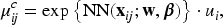
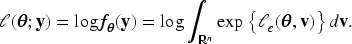
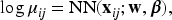
Let $y_{i j}$ denote a count output (response variable) and $x_{i j}$ denote corresponding $p$ -dimensional vector of input features (covariates), where the subscript $(i, j)$ indicates the $j$ th outcome of the $i$ th subject (or cluster) for $i = 1, \dots, n$ and $j = 1, \dots, q_{i}$ . For count outputs, Poisson neural network²⁰ gives the marginal predictor $η_{i j}^{m} = \log μ_{i j}^{m}$ ,

η_{i j}^{m} = NN (x_{i j}; w, β) = \sum_{k = 1}^{p_{L}} g_{k} (x_{i j}; w) β_{k} + β_{0},

(1)

where

μ_{i j}^{m} = E (Y_{i j} | x_{i j})

is the marginal mean, NN

(x_{i j}; w, β)

is a neural network predictor,

β = (β_{0}, β_{1}, \dots, β_{p_{L}})^{⊤}

is a vector of weights and bias between the last hidden layer and the output layer,

g_{k} (x_{i j}; w)

denotes the

k

-th node of the last hidden layer with a nonlinear activation function, and

w

is a vector of all the weights and biases before the last hidden layer. Here the bold face stands for vectors and matrices, while non-bold face stands for scalars. In Poisson neural network, the inverse of the log function,

\exp (\cdot)

, becomes the activation function of the output layer. Poisson neural networks allow highly nonlinear relationships between input and output variables, but only provide the marginal predictions for

μ_{i j}^{m}

. Thus, Poisson neural network can be viewed as an extension of Poisson GLM with

η_{i j}^{m} = x_{i j}^{⊤} β

2.2. PGNN

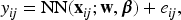
To allow subject-specific prediction into the model (1), we propose the PGNN,

η_{i j}^{c} = \log μ_{i j}^{c} = NN (x_{i j}; w, β) + z_{i j}^{⊤} v,

(2)

where

μ_{i j}^{c} = E (Y_{i j} | x_{i j}, v_{i})

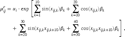
is the conditional mean,

NN (x_{i j}; w, β)

is the marginal predictor of the Poisson neural network (1),

v = (v_{1}, \dots, v_{n})^{⊤}

is the vector of random effects from the log-gamma distribution, and

z_{i j}

is a vector from the model matrix for random effects, representing the high-cardinality categorical features. The conditional mean

μ_{i j}^{c}

can be formulated as

μ_{i j}^{c} = \exp {NN (x_{i j}; w, β)} \cdot u_{i},

where

u_{i} = \exp (v_{i}) > 0

is the gamma random effect. For identifiability between the global intercept

β_{0}

and the random effects

v

, we impose the commonly-used constraints

E (u_{i}) = 1

.¹³ The use of constraints

E (u_{i}) = 1

has an advantage that the marginal predictions for the multiplicative model can be directly obtained, because

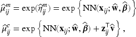
μ_{i j}^{m} = E [E (Y_{i j} | x_{i j}, u_{i})] = E [\exp {NN (x_{i j}; w, β)} \cdot u_{i}] = \exp {NN (x_{i j}; w, β)} .

Thus, we employ

v_{i} = \log u_{i}

to the model (2), where

u_{i} \sim Gamma (λ^{- 1}, λ^{- 1})

with

E (u_{i}) = 1

and

var (u_{i}) = λ

. By allowing two separate output nodes, the PGNN provides both marginal and subject-specific predictions,

\begin{aligned} {\hat{μ}}_{i j}^{m} & = \exp ({\hat{η}}_{i j}^{m}) = \exp {NN (x_{i j}; \hat{w}, \hat{β})} \\ {\hat{μ}}_{i j}^{c} & = \exp {NN (x_{i j}; \hat{w}, \hat{β}) + z_{i j}^{⊤} \hat{v}}, \end{aligned}

where the hats denote the predicted values. Subject-specific prediction can be achieved by multiplying the marginal mean predictor

{\hat{μ}}_{i j}^{m}

and the subject-specific predictor of random effect

{\hat{u}}_{i} = \exp ({\hat{v}}_{i})

. Here,

var (Y_{i j} | x_{i j}) = E [var (Y_{i j} | x_{i j}, v_{i})] + var [E (Y_{i j} | x_{i j}, v_{i}))] \geq E [var (Y_{i j} | x_{i j}, v_{i})],

where

var {E (Y_{i j} | x_{i j}, v_{i})}

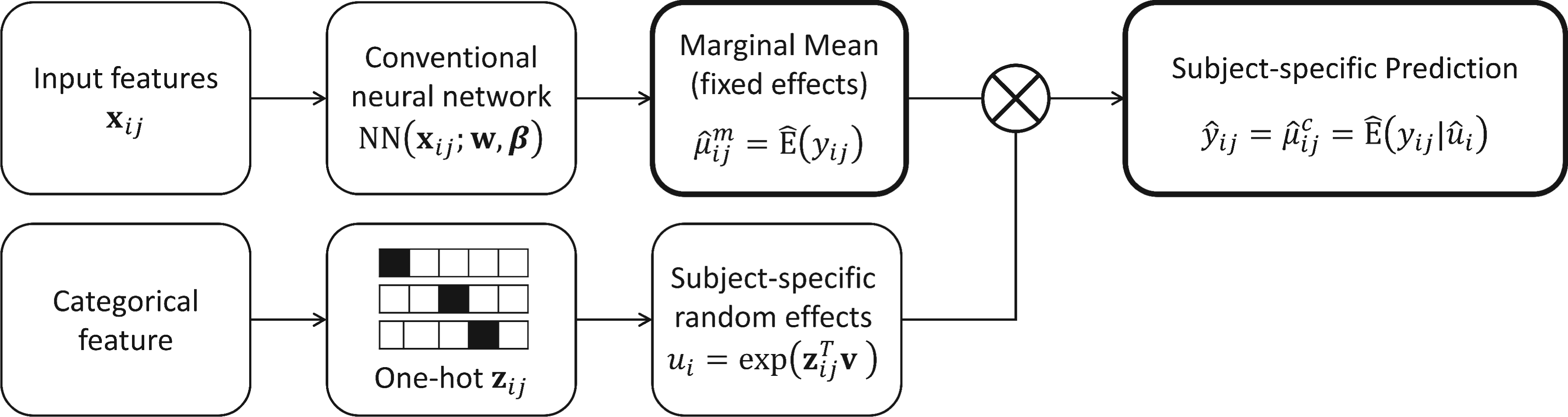
represents the between-subject variance and

E {var (Y_{i j} | x_{i j}, v_{i})}

represents the within-subject variance. To enhance the predictions, Poisson neural network improves the marginal predictor

μ_{i j}^{m} = E (Y_{i j} | x_{i j}) = E {E (Y_{i j} | x_{i j}, v_{i})}

by allowing highly nonlinear function of

x

, whereas PGNN further uses the conditional predictor

μ_{i j}^{c} = E (Y_{i j} | x_{i j}, v_{i})

, eliminating between-subject variance. Figure 1 illustrates an example of the proposed model architecture, including feature selection in Section 4. In particular, it has two separate output nodes for subject-specific predictions: the marginal mean

μ_{i j}^{m}

and the subject-specific random effects

v_{i}

. The proposed framework is architecture-agnostic with respect to the neural network component; in simulation studies, multi-layer perceptrons are adopted primarily to isolate the contribution of random effects without confounding architectural complexity.

Figure 1.

An example of the proposed model architecture. $x_{i j}$ denotes the input features (covariates), and $z_{i j}$ denotes an $n$ -dimensional one-hot encoded vector of a categorical feature, with the $i$ th entry equal to one and all remaining entries equal to zero. This representation bridges each observation $(i, j)$ to its corresponding random effect $u_{i}$ in the proposed model (2).

3. Construction of h-likelihood

For subject-specific prediction via random effects, this section primarily aims to define an objective function whose global maximizer corresponds to MLEs of fixed parameters $θ = (w, β, λ)$ . In the context of linear mixed models, Henderson et al.²¹ proposed to maximize the joint density with respect to fixed and random parameters. However, it cannot yield MLEs of variance components. There have been various attempts to extend joint maximization schemes with different justifications,^12,22–25 but failed to simultaneously obtain the MLEs of all fixed parameters and BUPs of random parameters by optimizing a single objective function. In Poisson-gamma HGLMs, Lee and Nelder³ proposed the use of an extended likelihood $ℓ_{e} (θ, v)$ ,

ℓ_{e} (θ, v) = \log f_{θ} (y, v) = \sum_{i, j} \log f_{w, β} (y_{i j} | v_{i}) + \sum_{i} \log f_{λ} (v_{i}),

(3)

where

f_{w, β} (y_{i j} | v_{i})

is the conditional probability density of

y_{i j} | v_{i}

and

f_{λ} (v_{i})

is the probability density of

v_{i}

. This objective function yields MLEs for

β

and BUPs for

u

through joint maximization, but does not provide an MLE for the variance component

λ

. In this paper, we derive the new h-likelihood whose joint maximization simultaneously yields MLEs of the whole fixed parameters including the variance component

λ

, BUPs of the random effects

u

, and conditional expectations

μ^{c} = (μ_{11}^{c}, \dots, μ_{n, q_{n}}^{c})^{⊤}

3.1. New h-likelihood for PGNN

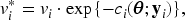
Suppose that $v^{*} = (v_{1}^{*}, \dots, v_{n}^{*})^{⊤}$ is a transformation of $v$ such that

v_{i}^{*} = v_{i} \cdot \exp {- c_{i} (θ; y_{i})},

where

c_{i} (θ; y_{i})

is a function of

θ

and

y_{i} = (y_{i 1}, \dots, y_{i q_{i}})^{⊤}

for

i = 1, 2, \dots, n

. Let

f_{θ} (v^{*} | y)

be the conditional probability density of

v^{*} | y

f_{θ} (y)

be the probability density of

y

, and

c (θ; y) = \sum_{i = 1}^{n} c_{i} (θ; y_{i})

. Then we define the h-likelihood as

h (θ, v) \equiv \log f_{θ} (v^{*} | y) + \log f_{θ} (y) = ℓ_{e} (θ, v) + c (θ; y),

(4)

if the joint maximization of

h (θ, v)

leads to MLEs of all the fixed parameters and BUPs of the random parameters. A sufficient condition for

h (θ, v)

to yield MLEs of all the fixed parameters in

θ

is that

{f_{θ} (v^{*} | y)}_{v^{*} = {\tilde{v}}^{*}}

, which is the value of the conditional density evaluated at the mode

v^{*} = {\tilde{v}}^{*}

, does not depend on

θ

, where the mode

{\tilde{v}}^{*}

{\tilde{v}}^{*} = {argmax}_{v^{*}} h (θ, v) = {argmax}_{v^{*}} \log f_{θ} (v^{*} | y) .

For the proposed PGNN, we found that the following function

c_{i} (θ; y_{i}) = y_{i +}^{*} + \log Γ (y_{i +}^{*}) - y_{i +}^{*} \log (y_{i +}^{*})

with

y_{i +}^{*} = \sum_{j = 1}^{q_{i}} y_{i j} + λ^{- 1}

satisfies the sufficient condition,

{\log f_{θ} (v^{*} | y)}_{v^{*} = {\tilde{v}}^{*}} = \sum_{i = 1}^{n} {\log f_{θ} (v_{i}^{*} | y)}_{v_{i}^{*} = {\tilde{v}}_{i}^{*}} = \sum_{i = 1}^{n} [{\log f_{θ} (v_{i} | y)}_{v_{i} = {\tilde{v}}_{i}} + c_{i} (θ; y_{i})] = 0,

where

{\tilde{v}}_{i} = {\tilde{v}}_{i}^{*} \cdot \exp {c_{i} (θ; y_{i})}

. Since

c_{i} (θ; y_{i})

only depends on

λ

and

y_{i +}

, we denote

c_{i} (θ; y_{i}) = c_{i} (λ; y_{i +}) .

Then, the h-likelihood at its mode,

h (θ, \tilde{v})

, becomes the classical (marginal) log-likelihood,

ℓ (θ; y) = \log f_{θ} (y) = \log \int_{R^{n}} \exp {ℓ_{e} (θ, v)} d v .

Thus, joint maximization of the h-likelihood (4) provides MLEs for all the fixed parameters

θ

, including the variance component

λ

, and BUPs of

u

\tilde{u} = \exp (\tilde{v}) = E (u | y),

which leads to the BUPs of conditional mean

μ^{c}

{\tilde{μ}}^{c} = \exp (\tilde{v}) \cdot \exp {NN (x; w, β)} = E (μ^{c} | y) .

The proof and technical details for the theoretical results are derived in Appendix A.1.

We note that the above theoretical results are established at the objective-function level. In practice, however, exact global maximization is generally infeasible in training neural networks based on stochastic optimization. Accordingly, the proposed learning algorithm described in Section 4 serves as a practical approximate optimization procedure.

3.2. Misspecification of the random effects distribution

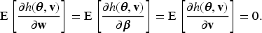
Since the random effects cannot be observed, checking the distributional assumption for random effects is often challenging in practice. This section demonstrates one advantage of the proposed method: the h-likelihood for PGNN is robust to misspecification of the random-effect distribution, in the sense that the corresponding estimating equations remain unbiased with respect to the mean components $w$ , $β$ , and $v$ under the constraint $E (u_{i}) = 1$ , even if the distribution of the random effects is misspecified. Consider the Poisson neural network with random effects $u_{i}$ such that $E (u_{i}) = 1$ , while the true distribution of $u_{i}$ is not gamma, that is, the distribution of $u_{i}$ is misspecified.

Theorem 1
For any distribution of $u_{i}$ under the constraints $E (u_{i}) = 1$ , the h-likelihood (4) satisfies
$E [\frac{\partial h (θ, v)}{\partial w}] = E [\frac{\partial h (θ, v)}{\partial β}] = E [\frac{\partial h (θ, v)}{\partial v}] = 0.$

Theorem 1 shows that the expected value of the score equations becomes zero, even if the distribution of $u$ is misspecified. Lee and Nelder²⁶ claimed that the robustness should be established by comparing like with like, that is, comparison for random effect predictors should be made under the common constraints $E (u_{i}) = 1$ . We further found that in practice, the proposed method maintains good prediction performance, even when the distributional assumption of random effects is violated. To confirm this, we include simulation studies with log-normal distributions and mixtures of log-normal distributions for $u_{i}$ in Section 5. In these cases, $u_{i}$ does not follow a gamma distribution, but the proposed method maintains the best performance in both scenarios, in terms of mean squared Pearson error and mean deviance. An additional simulation study illustrating the robustness of each parameter under misspecification of the random effects distribution is provided in Appendix C.1.
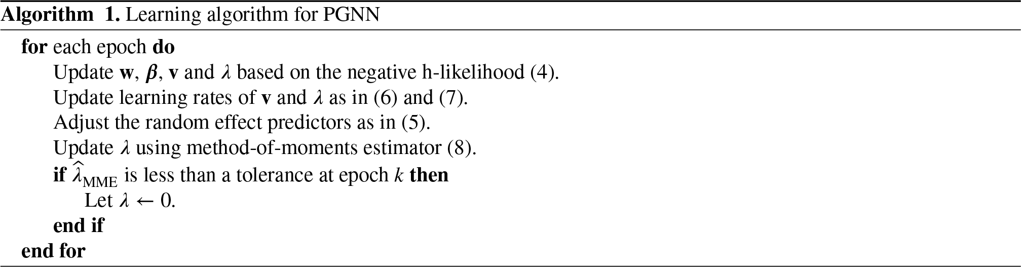
4. Learning algorithm for PGNN

In this section, we introduce the h-likelihood learning framework for handling count data with high-cardinality categorical features. Since exact global maximization of the proposed objective function is generally infeasible in stochastic neural-network training, we develop a practical approximate optimization procedure based on online learning. Specifically, we decompose the negative h-likelihood loss for online learning and propose additional procedures to improve predictive performance.

4.1. Loss function for online learning

The proposed PGNN can be trained by optimizing the negative h-likelihood loss with (4),

Loss = - h (θ, v)

which is a function of two separate output nodes

μ_{i j}^{m} = NN (x_{i j}; w, β)

and

v_{i} = z_{i j}^{⊤} v

. To apply online optimization methods, in each observation, the proposed loss function can be decomposed into

- h_{i j} = - y_{i j} (\log μ_{i j}^{m} + v_{i}) + e^{v_{i}} μ_{i j}^{m} - \frac{v_{i} - e^{v_{i}} - \log λ}{q_{i} λ} + \frac{\log Γ (λ^{- 1})}{q_{i}} - \frac{c_{i} (λ; y_{i +})}{q_{i}} .

Then, for each mini-batch

B

, the h-likelihood loss function is expressed as

{Loss}_{B} = - \sum_{(i, j) \in B} h_{i j} .

In our implementation, minibatches are formed by individual observations rather than by clusters for computational efficiency. The cluster-wise sum

y_{i +} = \sum_{j = 1}^{q_{i}} y_{i j}

c_{i} (λ; y_{i +})

is computed once from the training data prior to batch sampling.

4.2. Adjustment for random effects and variance component

While neural networks often encounter local minima, Dauphin et al.²⁷ claimed that in ordinary neural networks, local minima may not necessarily result in poor predictions. In contrast to HGLM and neural network, we observed that the local minima can lead to poor prediction when the network reflects subject-specific random effects. In PGNNs, we impose the constraint $E (u_{i}) = 1$ for identifiability between the global intercept $β_{0}$ and the random effects $v$ . However, in practice, PGNNs often end with local minima that violate the constraint. To prevent poor prediction due to local minima, we introduce an adjustment to the predictors of $u_{i}$ ,

{\hat{u}}_{i} \leftarrow \frac{{\hat{u}}_{i}}{\frac{1}{n} \sum_{i = 1}^{n} {\hat{u}}_{i}} and {\hat{β}}_{0} \leftarrow {\hat{β}}_{0} + \log (\sum_{i = 1}^{n} \frac{{\hat{u}}_{i}}{n})

(5)

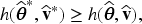
to satisfy

\sum_{i = 1}^{n} {\hat{u}}_{i} / n = 1

. Note that this adjustment is introduced primarily to stabilize optimization and improve convergence, rather than to provide identifiability guaranties for all neural network parameters, which are typically not identifiable in a strict sense in neural networks. The following theorem shows that the proposed adjustment improves the local h-likelihood prediction. The proof is given in Appendix A.3.

Theorem 2

In PGNNs, suppose that ${\hat{β}}_{0}$ and ${\hat{u}}_{i}$ are estimates of $β_{0}$ and $u_{i}$ such that $\sum_{i = 1}^{n} {\hat{u}}_{i} / n = 1 + ϵ$ for some $ϵ \in R$ . Let ${\hat{u}}_{i}^{*}$ and ${\hat{β}}_{0}^{*}$ be the adjusted estimators in (5). Then,

h ({\hat{θ}}^{*}, {\hat{v}}^{*}) \geq h (\hat{θ}, \hat{v}),

and the equality holds if and only if

ϵ = 0

, where

\hat{θ}

and

{\hat{θ}}^{*}

are vectors of the same fixed parameter estimates but with different

{\hat{β}}_{0}

and

{\hat{β}}_{0}^{*}

for

β_{0}

, respectively.

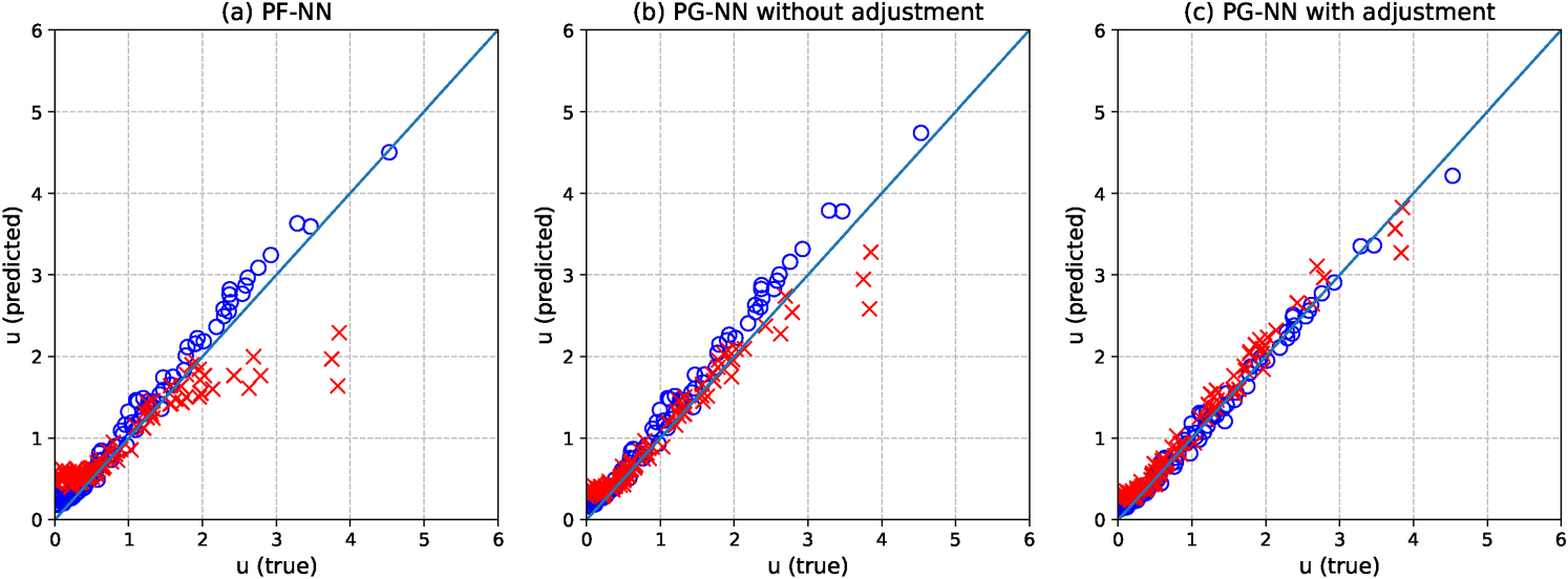
Theorem 2 shows that the adjustment (5) improves the random effect prediction. According to our experience, even though limited, this adjustment becomes important, especially when the cluster size is large. We presented two replications for visualization in Figure 2, which is the plot of ${\hat{u}}_{i}$ against the true $u_{i}$ under $(n, q) = (100, 100)$ and $λ = 1$ . Figure 2 (a) shows that the use of fixed effects for subject-specific effects (Poisson-NN(c)) produces poor prediction of $u_{i}$ . Figure 2 (b) and (c) show that the use of random effects for subject-specific effects (PGNN) improves the subject-specific prediction, and the proposed adjustment improves it further. Based on 100 replications, the RMSE of the random effect $u_{i}$ ’s are 0.28 (PF-NN), 0.25 (PG-NN without adjustment), 0.14 (PG-NN with adjustment). Thus, the proposed adjustment significantly enhances prediction accuracy of subject-specific effects.

Figure 2.

Predicted values of $u_{i}$ from two replications (marked as o and x for each) when $u_{i}$ is generated from the Gamma distribution with $λ = 1$ , $n = 100$ , $q = 100$ .

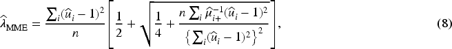
We further found that estimation of the variance component $λ = var (u_{i})$ could be sensitive in the early stage of learning, because $\hat{λ}$ could converge to zero when $\hat{v} \approx 0$ in the early stage and $\hat{v}$ could converge to zero when $\hat{λ} \approx 0$ . To improve the algorithm, we introduce a warm-up stage based on cosine annealing learning rate,²⁸

\begin{aligned} learning rate of v = 1.5 + 0.5 \cos (π \cdot epoch / k) \end{aligned}

(6)

\begin{aligned} learning rate of λ = 0.5 - 0.5 \cos (π \cdot epoch / k) \end{aligned}

(7)

until

epoch < k

for a predetermined number of warm-up epochs

k

. At the end of warm-up stage, we introduce a cut-off procedure for sparsity: if

\hat{λ}

is less than a certain value, then let

\hat{λ} = 0

. We further propose the use of the method-of-moments estimator (MME) in early stage for this procedure,

{\hat{λ}}_{MME} = \frac{\sum_{i} ({\hat{u}}_{i} - 1)^{2}}{n} [\frac{1}{2} + \sqrt{\frac{1}{4} + \frac{n \sum_{i} {\hat{μ}}_{i +}^{- 1} ({\hat{u}}_{i} - 1)^{2}}{{\sum_{i} ({\hat{u}}_{i} - 1)^{2}}^{2}}}],

(8)

where

{\hat{μ}}_{i +} = \sum_{j = 1}^{q_{i}} {\hat{μ}}_{i j}^{m}

. Convergence of the MME (8) is shown in Appendix A.4. In Appendix C.4, we demonstrate an additional experiment for verifying the consistency of

\hat{λ}

of the proposed method. The entire learning algorithm of the proposed method is summarized in Algorithm 1. A hyperparameter sensitivity analysis for the learning algorithm is reported in Appendix C.3, suggesting stable performance across a range of learning rates and warm-up settings, with minor degradation for small batch sizes.

5. Simulation studies

5.1. Data generation

To investigate the practical robustness of the proposed method to misspecification of the random effects distribution, random effects are generated from the following distributions:

Constant: $u_{i} = 1$ (i.e. $v_{i} = \log u_{i} = 0$ ) for all $i = 1, \dots, n$ and $λ = Var (u_{i}) = 0$ . The true model does not have random effects, hence the conditional mean $μ_{i j}^{c}$ is identical to marginal mean $μ_{i j}^{m}$ .

Gamma: G $(λ)$ indicates that $u_{i}$ is generated from a gamma distribution with mean 1 and variance $λ$ , which corresponds to the model assumption.

Log-normal: LN $(λ)$ indicates that $u_{i}$ is generated from a log-normal distribution with mean 1 and variance $λ$ , that is, $\log u_{i}$ follows a normal distribution. Compared to the gamma distribution, the log-normal distribution exhibits slightly heavier tail behavior and is therefore used to assess robustness under heavy-tailed random-effects misspecification.

Inverse-gamma: IG $(λ)$ indicates that $u_{i}$ is generated from an inverse-gamma distribution with mean 1 and variance $λ$ . This scenario represents another positive heavy-tailed alternative to the gamma distribution and is considered to assess robustness under tail misspecification.

Mixture: Mix $(λ)$ indicates that $u_{i}$ is generated from a mixture of two log-normal distributions, where $u_{i} = u_{i 1}$ with probability $1 / 2$ and $u_{i} = u_{i 2}$ with probability $1 / 2$ . Here, $u_{i 1}$ and $u_{i 2}$ are independently generated from log-normal distributions with $E (u_{i 1}) = 0.5$ , $Var (u_{i 1}) = (4 λ - 1) / 20$ , and $E (u_{i 2}) = 1.5$ , $Var (u_{i 2}) = 9 (4 λ - 1) / 20$ , as in Ha and Lee.²⁹ This scenario yields a bimodal random-effects distribution that is structurally far from the gamma distribution and is designed to assess robustness under pronounced distributional misspecification.

Contaminated: This indicates a contamination scenario in which the response variable $Y_{i j}$ is generated from a Poisson distribution with mean $μ_{i j}$ under the baseline scenario G(1), and a small fraction (5%) of observations in the upper tail are artificially inflated by an additive constant of 5. This setting introduces observation-level misspecification and is used to assess robustness against outlier contamination that deviates from the Poisson assumption.

We generate

p = 50

dimensional input features

x_{i j}

from multivariate normal distributions with zero means and covariance structures; independent, AR(1), AR(2), compound symmetry (CS), and a mixture of AR(1) and CS. The output variable

y_{i j}

is generated from

Poisson (μ_{i j}^{c})

with the following nonlinear conditional mean:

\begin{aligned} μ_{i j}^{c} & = u_{i} \cdot \exp [\sum_{k = 1}^{10} \sin (x_{i j, k}) β_{k} + \sum_{k = 10}^{20} \cos (x_{i j, k}) β_{k} \\ + \sum_{k = 20}^{30} \sin (x_{i j, k} x_{i j, k + 10}) β_{k} + \sum_{k = 30}^{40} \cos (x_{i j, k} x_{i j, k + 10}) β_{k}], \end{aligned}

where

x_{i j, k}

and

β_{k}

are the

k

-th components of the input vector

x_{i j}

and the parameter vector

β = (- 0.1, - 0.08, \dots, - 0.02, 0.02, \dots, 0.1)^{⊤}

, respectively. The data size is

N = 120

K with the number of subjects (the cardinality of the categorical features)

n = 10

K and the number of repeated measures (cluster size)

q = 12

. Then, for each subject

i

, we assigned 8 observations

(j = 1, \dots, 8)

to the training set, 2 observations

(j = 9, 10)

to the validation set, and the remaining 2 observations

(j = 11, 12)

to the test set.

5.2. Existing models

We compare the predictive performance of the PGNN with the following methods, including state-of-the-art methods for clustered data. For simulation studies, we also present the predictive performance of the true mean $μ_{i j}$ .

Gaussian-NN(m) is a conventional neural network for continuous outputs, which can be expressed as

y_{i j} = NN (x_{i j}; w, β) + e_{i j},

where

e_{i j} \sim N (0, σ_{e}^{2})

is a white noise. This model gives marginal predictions

{\hat{μ}}_{i j}^{m} = NN (x_{i j}; \hat{w}, \hat{β})

Gaussian-NN(c) is a neural network with fixed subject-specific effects for continuous outputs, which can be expressed as

y_{i j} = NN (x_{i j}; w, β) + v_{i} + e_{i j},

where

v_{i}

is a fixed parameter for

i

-th subject and

e_{i j} \sim N (0, σ_{e}^{2})

is a random noise. This model gives subject-specific predictions

{\hat{μ}}_{i j}^{c} = NN (x_{i j}; \hat{w}, \hat{β}) + {\hat{v}}_{i}

, where all the parameters are estimated by maximizing

\log f_{w, β, v} (y)

Poisson-NN(m) is a conventional neural network for count outputs, which can be expressed as

\log μ_{i j} = NN (x_{i j}; w, β),

where

y_{i j} \sim Poisson (μ_{i j})

. This model gives marginal predictions

{\hat{μ}}_{i j}^{m} = \exp {NN (x_{i j}; \hat{w}, \hat{β})}

Poisson-NN(c) is a neural network with fixed subject-specific effects for count outputs, which can be expressed as

\log μ_{i j} = NN (x_{i j}; w, β) + v_{i},

where

v_{i}

is a fixed parameter for

i

-th subject and

y_{i j} \sim Poisson (μ_{i j})

. This model gives subject-specific predictions

{\hat{μ}}_{i j}^{c} = \exp {NN (x_{i j}; \hat{w}, \hat{β}) + {\hat{v}}_{i}}

, where all the parameters are estimated by maximizing

\log f_{w, β, v} (y)

LMMNN^5,6 is one of the state-of-the-art model for clustered continuous data. This model can be expressed as

y_{i j} = NN (x_{i j}; w, β) + v_{i} + e_{i j},

where

v_{i}

is a random effect for

i

-th subject and

e_{i j} \sim N (0, σ_{e}^{2})

is a white noise. This model gives subject-specific predictions

{\hat{μ}}_{i j}^{c} = \exp {NN (x_{i j}; \hat{w}, \hat{β}) + {\hat{v}}_{i}}

, where the fixed parameters are estimated by maximizing the marginal likelihood

\log f_{w, β} (y)

and the random effects are predicted by the BUPs. For the application of stochastic optimization methods, Simchoni and Rosset⁶ proposed the use of block-diagonal approximation to the marginal covariance.

H-LMMNN⁷ is another state-of-the-art model for clustered continuous data. The model equation is the same with LMMNN,

y_{i j} = NN (x_{i j}; w, β) + v_{i} + e_{i j},

where

v_{i}

is a random effect for

i

-th subject and

e_{i j} \sim N (0, σ_{e}^{2})

is a white noise. However, the estimators of fixed parameters and the predictors of random effects are simultaneously obtained by optimizing the h-likelihood. When the random effects are highly correlated, H-LMMNN would be preferred to LMMNN since it does not require approximation methods.

PGNN-A is the proposed models for clustered count outputs in Section 2.2 with the adjustment procedure for random effects and variance component in Section 4.2. PGNN-N is the proposed model without the adjustment procedure, considered for the ablation study. They can be expressed as

\log μ_{i j} = NN (x_{i j}; w, β) + \log u_{i},

where

y_{i j} | u_{i} \sim Poisson (μ_{i j})

and

u_{i} \sim Gamma (1 / λ, 1 / λ)

, based on the proposed h-likelihood method described in Sections 3 and 4. This model gives subject-specific predictions

{\hat{μ}}_{i j}^{c} = \exp {NN (x_{i j}; \hat{w}, \hat{β}) + \log {\hat{u}}_{i}}

We employed the same architecture for all neural networks with a standard multi-layer perceptron (MLP) consisting of three hidden layers of [50, 25, 12] nodes and the LeakyReLU activation function. For Gaussian models, we applied log-transformation

\log (y_{i j} + 0.5)

for training and take exponential

{\exp ({\hat{y}}_{i j}) - 0.5}

for prediction. We applied the Adam optimizer with a learning rate of 0.01 and a batch size of 1000 and an early stopping process based on the validation loss with patience 5. LMMNN was implemented in Python using Keras³⁰ and TensorFlow³¹ and the other neural network-based models were implemented in PyTorch.³² NVIDIA A100 GPUs were used for computations.

5.3. Results

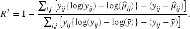
To evaluate the prediction performances, we consider the root mean of squared Pearson error (RMSPE) and the root mean of deviance (RMD),

RMSPE = \sqrt{\frac{1}{N} \sum_{i, j} \frac{(y_{i j} - {\hat{μ}}_{i j})^{2}}{V ({\hat{μ}}_{i j})}} and RMD = \sqrt{\frac{1}{N} \sum_{i, j} [y_{i j} {\log (y_{i j}) - \log ({\hat{μ}}_{i j})} - (y_{i j} - {\hat{μ}}_{i j})]}

Here,

V (μ_{i j})

is defined by either

Var (y_{i j} | u_{i}) = ϕ V (μ_{i j})

with

μ_{i j} = μ_{i j}^{c}

for conditional models or

Var (y_{i j}) = ϕ V (μ_{i j})

with

μ_{i j} = μ_{i j}^{m}

for marginal models, where

ϕ

is a dispersion parameter of the GLM family. For normal outputs, the RMSPE is identical to the ordinary root mean squared error, since

ϕ = σ^{2}

and

V (μ_{i j}^{c}) = 1

. For Poisson outputs,

ϕ = 1

and

V (μ_{i j}^{c}) = μ_{i j}^{c}

. In Appendix, we further present confidence intervals, computing times, and deviance

R^{2}

for count data,

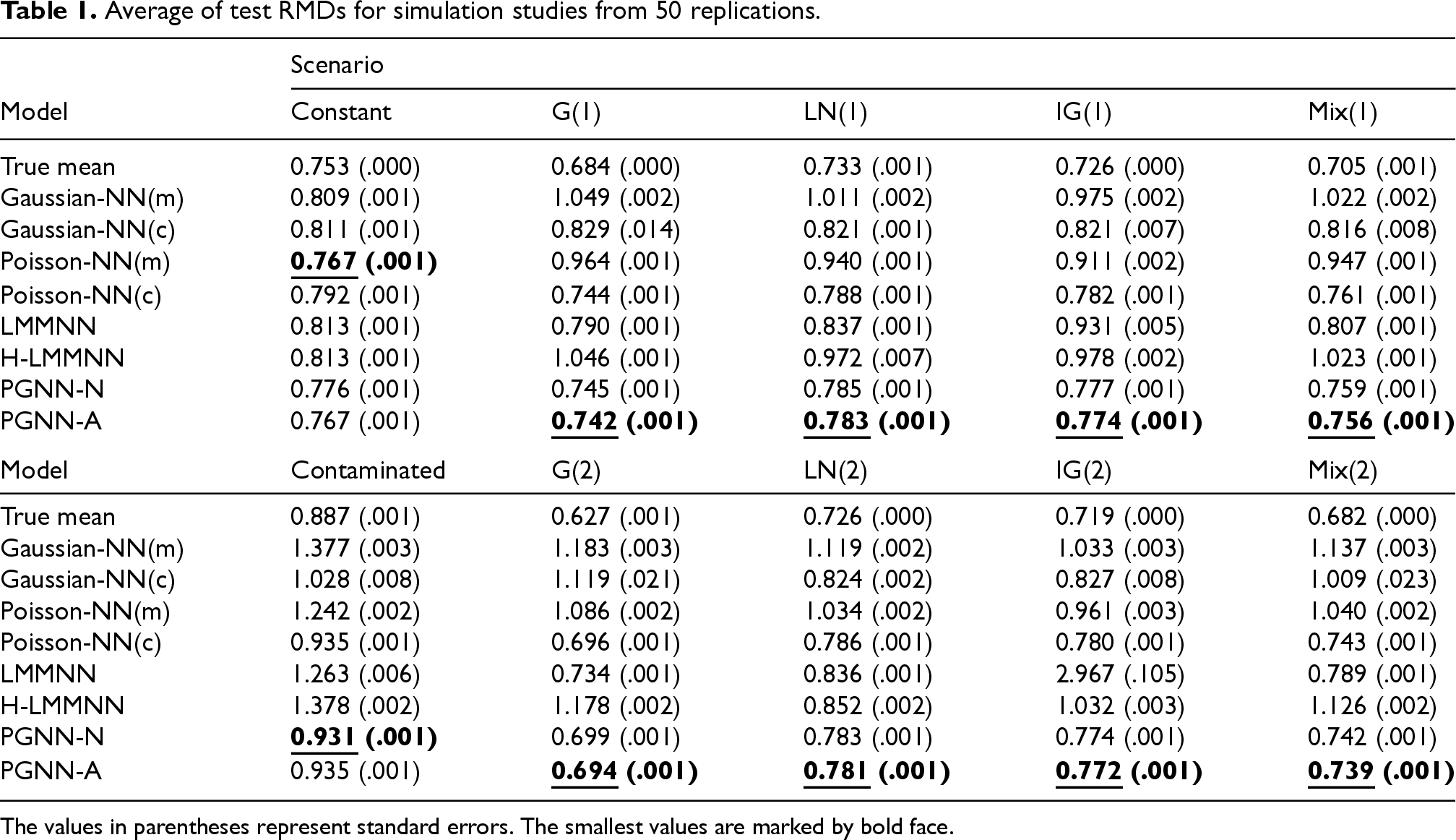
R^{2} = 1 - \frac{\sum_{i, j} [y_{i j} {\log (y_{i j}) - \log ({\hat{μ}}_{i j})} - (y_{i j} - {\hat{μ}}_{i j})]}{\sum_{i, j} [y_{i j} {\log (y_{i j}) - \log (\bar{y})} - (y_{i j} - \bar{y})]} .

Table 1.
Average of test RMDs for simulation studies from 50 replications.

Scenario

Model Constant G(1) LN(1) IG(1) Mix(1)

True mean 0.753 (.000) 0.684 (.000) 0.733 (.001) 0.726 (.000) 0.705 (.001)

Gaussian-NN(m) 0.809 (.001) 1.049 (.002) 1.011 (.002) 0.975 (.002) 1.022 (.002)

Gaussian-NN(c) 0.811 (.001) 0.829 (.014) 0.821 (.001) 0.821 (.007) 0.816 (.008)

Poisson-NN(m) 0.767 (.001) 0.964 (.001) 0.940 (.001) 0.911 (.002) 0.947 (.001)

Poisson-NN(c) 0.792 (.001) 0.744 (.001) 0.788 (.001) 0.782 (.001) 0.761 (.001)

LMMNN 0.813 (.001) 0.790 (.001) 0.837 (.001) 0.931 (.005) 0.807 (.001)

H-LMMNN 0.813 (.001) 1.046 (.001) 0.972 (.007) 0.978 (.002) 1.023 (.001)

PGNN-N 0.776 (.001) 0.745 (.001) 0.785 (.001) 0.777 (.001) 0.759 (.001)

PGNN-A 0.767 (.001) 0.742 (.001) 0.783 (.001) 0.774 (.001) 0.756 (.001)

Model Contaminated G(2) LN(2) IG(2) Mix(2)

True mean 0.887 (.001) 0.627 (.001) 0.726 (.000) 0.719 (.000) 0.682 (.000)

Gaussian-NN(m) 1.377 (.003) 1.183 (.003) 1.119 (.002) 1.033 (.003) 1.137 (.003)

Gaussian-NN(c) 1.028 (.008) 1.119 (.021) 0.824 (.002) 0.827 (.008) 1.009 (.023)

Poisson-NN(m) 1.242 (.002) 1.086 (.002) 1.034 (.002) 0.961 (.003) 1.040 (.002)

Poisson-NN(c) 0.935 (.001) 0.696 (.001) 0.786 (.001) 0.780 (.001) 0.743 (.001)

LMMNN 1.263 (.006) 0.734 (.001) 0.836 (.001) 2.967 (.105) 0.789 (.001)

H-LMMNN 1.378 (.002) 1.178 (.002) 0.852 (.002) 1.032 (.003) 1.126 (.002)

PGNN-N 0.931 (.001) 0.699 (.001) 0.783 (.001) 0.774 (.001) 0.742 (.001)

PGNN-A 0.935 (.001) 0.694 (.001) 0.781 (.001) 0.772 (.001) 0.739 (.001)

	Scenario
True mean	0.753 (.000)	0.684 (.000)	0.733 (.001)	0.726 (.000)	0.705 (.001)
Gaussian-NN(m)	0.809 (.001)	1.049 (.002)	1.011 (.002)	0.975 (.002)	1.022 (.002)
Gaussian-NN(c)	0.811 (.001)	0.829 (.014)	0.821 (.001)	0.821 (.007)	0.816 (.008)
Poisson-NN(m)	0.767 (.001)	0.964 (.001)	0.940 (.001)	0.911 (.002)	0.947 (.001)
Poisson-NN(c)	0.792 (.001)	0.744 (.001)	0.788 (.001)	0.782 (.001)	0.761 (.001)
LMMNN	0.813 (.001)	0.790 (.001)	0.837 (.001)	0.931 (.005)	0.807 (.001)
H-LMMNN	0.813 (.001)	1.046 (.001)	0.972 (.007)	0.978 (.002)	1.023 (.001)
PGNN-N	0.776 (.001)	0.745 (.001)	0.785 (.001)	0.777 (.001)	0.759 (.001)
PGNN-A	0.767 (.001)	0.742 (.001)	0.783 (.001)	0.774 (.001)	0.756 (.001)
Model	Contaminated	G(2)	LN(2)	IG(2)	Mix(2)
True mean	0.887 (.001)	0.627 (.001)	0.726 (.000)	0.719 (.000)	0.682 (.000)
Gaussian-NN(m)	1.377 (.003)	1.183 (.003)	1.119 (.002)	1.033 (.003)	1.137 (.003)
Gaussian-NN(c)	1.028 (.008)	1.119 (.021)	0.824 (.002)	0.827 (.008)	1.009 (.023)
Poisson-NN(m)	1.242 (.002)	1.086 (.002)	1.034 (.002)	0.961 (.003)	1.040 (.002)
Poisson-NN(c)	0.935 (.001)	0.696 (.001)	0.786 (.001)	0.780 (.001)	0.743 (.001)
LMMNN	1.263 (.006)	0.734 (.001)	0.836 (.001)	2.967 (.105)	0.789 (.001)
H-LMMNN	1.378 (.002)	1.178 (.002)	0.852 (.002)	1.032 (.003)	1.126 (.002)
PGNN-N	0.931 (.001)	0.699 (.001)	0.783 (.001)	0.774 (.001)	0.742 (.001)
PGNN-A	0.935 (.001)	0.694 (.001)	0.781 (.001)	0.772 (.001)	0.739 (.001)

The values in parentheses represent standard errors. The smallest values are marked by bold face.

Table 2.

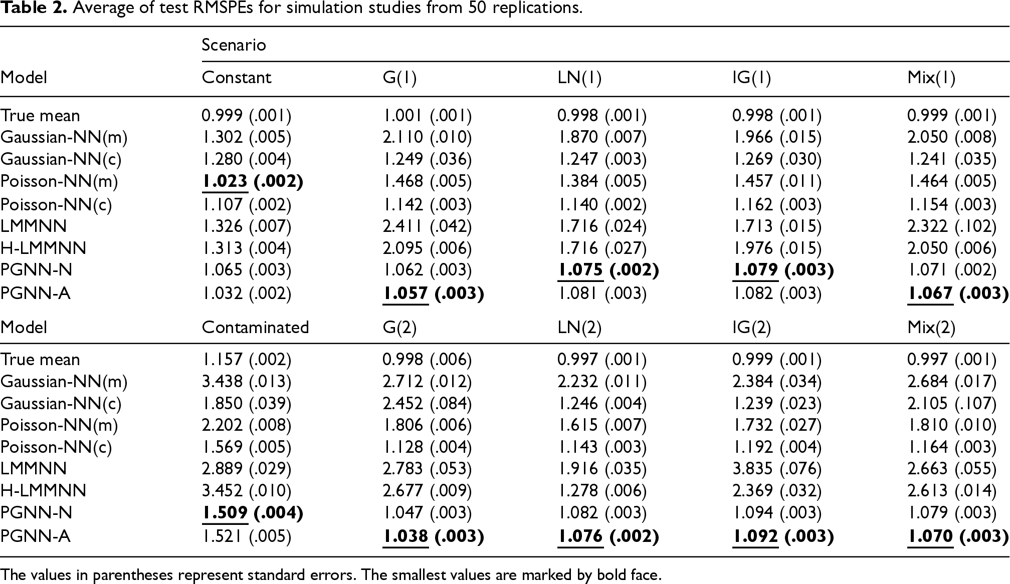
Average of test RMSPEs for simulation studies from 50 replications.

	Scenario
Model	Constant	G(1)	LN(1)	IG(1)	Mix(1)
True mean	0.999 (.001)	1.001 (.001)	0.998 (.001)	0.998 (.001)	0.999 (.001)
Gaussian-NN(m)	1.302 (.005)	2.110 (.010)	1.870 (.007)	1.966 (.015)	2.050 (.008)
Gaussian-NN(c)	1.280 (.004)	1.249 (.036)	1.247 (.003)	1.269 (.030)	1.241 (.035)
Poisson-NN(m)	1.023 (.002)	1.468 (.005)	1.384 (.005)	1.457 (.011)	1.464 (.005)
Poisson-NN(c)	1.107 (.002)	1.142 (.003)	1.140 (.002)	1.162 (.003)	1.154 (.003)
LMMNN	1.326 (.007)	2.411 (.042)	1.716 (.024)	1.713 (.015)	2.322 (.102)
H-LMMNN	1.313 (.004)	2.095 (.006)	1.716 (.027)	1.976 (.015)	2.050 (.006)
PGNN-N	1.065 (.003)	1.062 (.003)	1.075 (.002)	1.079 (.003)	1.071 (.002)
PGNN-A	1.032 (.002)	1.057 (.003)	1.081 (.003)	1.082 (.003)	1.067 (.003)
Model	Contaminated	G(2)	LN(2)	IG(2)	Mix(2)
True mean	1.157 (.002)	0.998 (.006)	0.997 (.001)	0.999 (.001)	0.997 (.001)
Gaussian-NN(m)	3.438 (.013)	2.712 (.012)	2.232 (.011)	2.384 (.034)	2.684 (.017)
Gaussian-NN(c)	1.850 (.039)	2.452 (.084)	1.246 (.004)	1.239 (.023)	2.105 (.107)
Poisson-NN(m)	2.202 (.008)	1.806 (.006)	1.615 (.007)	1.732 (.027)	1.810 (.010)
Poisson-NN(c)	1.569 (.005)	1.128 (.004)	1.143 (.003)	1.192 (.004)	1.164 (.003)
LMMNN	2.889 (.029)	2.783 (.053)	1.916 (.035)	3.835 (.076)	2.663 (.055)
H-LMMNN	3.452 (.010)	2.677 (.009)	1.278 (.006)	2.369 (.032)	2.613 (.014)
PGNN-N	1.509 (.004)	1.047 (.003)	1.082 (.003)	1.094 (.003)	1.079 (.003)
PGNN-A	1.521 (.005)	1.038 (.003)	1.076 (.002)	1.092 (.003)	1.070 (.003)

The values in parentheses represent standard errors. The smallest values are marked by bold face.

Tables 1 and 2 show the means and standard errors of test RMSPEs and RMDs from the simulation studies, respectively. When the true model has random effects, the proposed PGNNs significantly outperform the other models in terms of RMSPE and RMD, regardless of the true distribution of random effects. When the true model does not have random effects ( $u_{i} = 1$ is constant for all $i$ ), as expected, Poisson-NN(m) is the closest to the true model, hence it performs the best. However, the proposed model PGNN-A is comparable to Poisson-NN(m) even in this scenario, where the difference is not significant at significance level $0.05$ . Even when the distribution of random effects is misspecified in the scenarios LN(1), LN(2), Mix(1) and Mix(2), PGNNs still performs the best, in accordance with the theoretical findings in Section 3.2. Comparison of PGNN-N and PGNN-A illustrates that the adjustment procedure for random effects and variance component in Section 4.2 can improve the prediction performance in terms of RMSPE and RMD. Appendix C.2 presents more detailed results for comparison of PGNN-A and PGNN-N.

5.4. Correlated random effects

To further examine the behavior of the proposed method under more challenging dependence structures, we consider an additional scenario with correlated random effects. This setting is used to illustrate the applicability of the proposed framework to random effects with a correlation structure.

To accommodate correlated random effects within the proposed neural-network-based formulation, we introduce an additional hidden layer acting on the one-hot encoded input $z_{i j}$ . This modifies the subject-specific component $Z v$ in the network predictor $η$ to $Z L v$ , where $v$ is assumed to be independent. We then impose the constraint that the weight matrix $L$ of the added layer is a lower triangular matrix satisfying $λ L L^{⊤} = Σ$ , where $Σ$ represents the prespecified covariance structure for random effects. This construction extends the proposed framework to incorporate correlated random effects. For numerical evaluation, we consider the following scenario.

AR: AR scenario generates $v_{i} = \log u_{i}$ from a multivariate normal distribution with an AR(1) covariance structure and a correlation parameter $ρ = 0.5$ . The mean and marginal variance of $v_{i}$ are matched to those of the LN(1) scenario, so that $E (u_{i}) = 1$ and $Var (u_{i}) = 1$ . This scenario introduces dependence among the random effects to assess the applicability of the proposed method to correlated random effects.

For simulation data generated under the AR scenario, the covariance matrix of random effects is modeled using an AR(1) correlation kernel with unknown correlation parameter

ρ

and variance component

λ

. Both

ρ

and

λ

are estimated from the data jointly with other model parameters. The averages (standard errors) of the RMDs and RMSPEs for the proposed method are 0.784 (0.001) and 1.069 (0.002), respectively, while those for the true model are 0.734 (0.000) and 1.001 (0.001). The average of the estimated

ρ

is 0.370 (0.003), which slightly underestimates the true value.

The observed underestimation of $ρ$ suggests a mild shrinkage toward independence. A similar tendency toward underestimation has also been reported in neural network models for correlated Gaussian data.⁶ One possible explanation is that stochastic optimization, which relies on mini-batches rather than the full data, may adversely affect the estimation of between-cluster correlation structures. In addition, correlation parameters are often initialized near independence ( $ρ = 0$ ), which may further contribute to this tendency. To alleviate this issue, one may consider alternative batch sampling strategies designed to increase the probability that observations from neighboring clusters are included within the same mini-batch. Investigation of such strategies for improving variance component estimation is beyond the scope of the current paper and remains an interesting direction for future research. Nevertheless, prediction accuracy remains largely unaffected, suggesting that the proposed method can still provide reliable predictions despite moderate bias in the estimate of $ρ$ .

6. Real data analysis

Longitudinal data and clustered data are widely used in biomedical studies. In longitudinal data, predictions for future trend or status of subject outcomes are of interest. In clustered data, tailored predictions for specific clusters, such as hospitals and patient cohorts, are of interest, as they allow for more efficient resource allocation.¹¹ We investigate the prediction performance of the proposed method compared to existing methods, which is an important evaluation procedure for predicting future outcomes in clustered count data.

We examine the five real datasets below, including three longitudinal medical datasets and two clustered biological datasets. These datasets exhibit subject-specific (or cluster-specific) effects and include high-cardinality categorical features relative to the sample sizes. The real datasets were intentionally chosen to represent a wide range of data regimes, including cases where the advantages of neural-network-based models may be limited, in order to provide a balanced assessment of the proposed method in diverse practical scenarios. In particular, the proposed method is expected to offer greater flexibility in large-scale datasets with complex nonlinear patterns, such as the CD4 data, whereas classical GLMMs may remain competitive in settings with limited sample sizes or approximately linear structures, such as the Epilepsy data.

Epilepsy data: Epilepsy data are reported in Thall and Vail¹⁸ from a clinical trial of $n = 59$ patients with epilepsy. The data contain $N = 236$ observations with $q_{i} = 4$ repeated measures from each patient. The response variable $Y$ is the number of seizures occurring over the previous two weeks, measured at each of four successive post-randomization clinic visits. The primary interest is to predict the number of seizures over time for each patient. The dataset is available in epil data of the R package MASS³³ at http://doi.org/10.32614/CRAN.package.MASS.

CD4 data: CD4 data are from a study of AIDS patients with advanced immune suppression, reported in Henry et al.¹⁹ The data contain $N = 4612$ observations from $n = 1036$ patients with $q_{i} \geq 2$ repeated measurements. The response variable $Y$ is the longitudinal CD4 cell count. The primary interest is to predict the evolution of CD4 counts over time for each patient. The dataset is available in aidscd4 data of the R package bcmixed³⁴ at http://doi.org/10.32614/CRAN.package.bcmixed.

Bolus data: Bolus data are from a clinical trial following abdominal surgery, reported in Henderson and Shimakura.¹⁷ The data contain $N = 780$ observations for $n = 65$ patients with $q_{i} = 12$ repeated measurements. The response variable $Y$ is the number of analgesic doses taken by hospital patients in 12 successive four-hourly intervals. The primary interest is to predict the longitudinal trajectory of $Y$ over time. The dataset is available in bolus data of the R package cold³⁵ at http://doi.org/10.32614/CRAN.package.cold.

Owls data: Owls data are reported in Roulin and Bersier.¹⁶ The data contain $N = 599$ observations for $n = 27$ nests, with cluster sizes $q_{i}$ ranging from 4 to 52. The response variable $Y$ is number of negotiations per chick, representing the intensity of begging behavior. The primary interest is to predict begging intensity. The dataset is available in Owls data of the R package glmmTMB³⁶ at http://doi.org/10.32614/CRAN.package.glmmTMB.

Fruits data: Fruits data are reported in Banta et al.³⁷ The data have $N = 625$ observations clustered by $n = 24$ maternal seed families, with cluster sizes $q_{i}$ ranging from 11 to 47. The response variable $Y$ is the total number of fruits produced per plant. The primary interest is to predict reproductive output. The dataset is available in Arabidopsis data of the R package lme4³⁸ at http://doi.org/10.32614/CRAN.package.lme4.

For all datasets, we performed 10-fold cross-validation. Longitudinal data are treated as special cases of clustered data in which observations possess an inherent temporal ordering. We employed standard MLPs with 2 hidden layers for network architectures and LeakyReLU activation for all considered methods. The hyperparameters were selected from small candidate sets based on predictive performance on the training data, and the same selection procedure was applied consistently across all neural-network-based methods and datasets. We considered a number of nodes in

{4, 8}

, batch sizes in

{16, 32}

, learning rates in

{0.001, 0.01}

, and early stopping criteria with patience 5. For real data analyses with small-to-moderate sample sizes, we included Poisson-based linear models (Poisson-GLM and Poisson-GLMM) implemented in R. However, Poisson-GLMM could not be implemented in simulation studies due to the scalability issue.

Table 3.
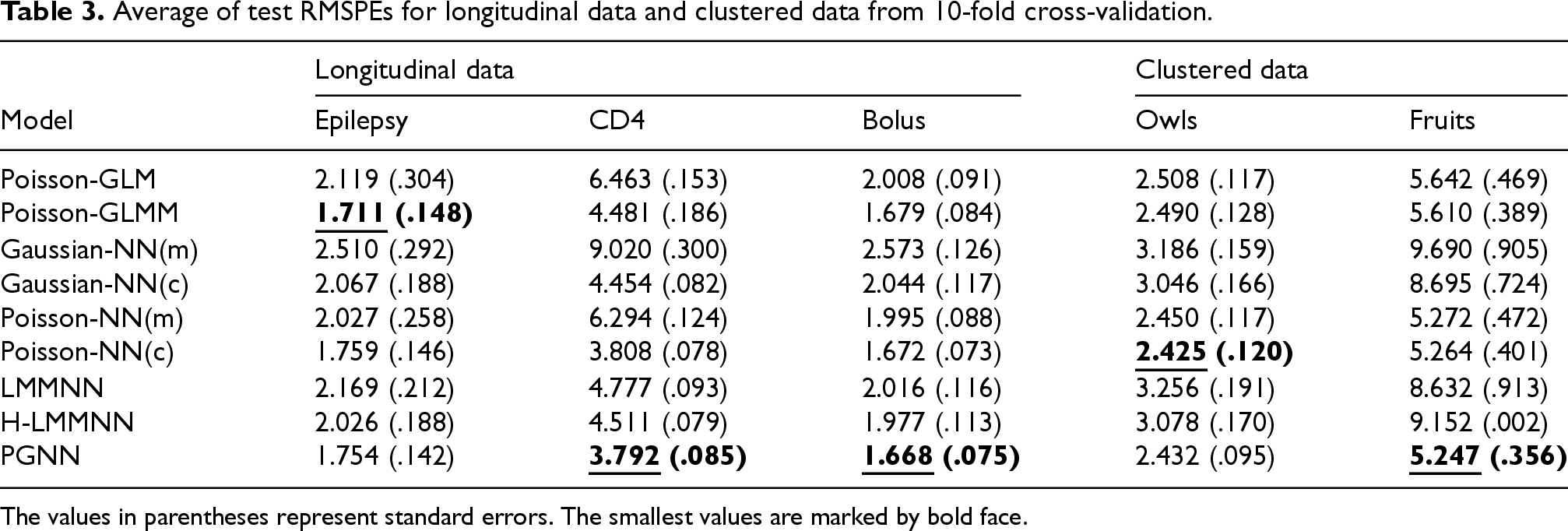
Average of test RMSPEs for longitudinal data and clustered data from 10-fold cross-validation.

Longitudinal data Clustered data

Model Epilepsy CD4 Bolus Owls Fruits

Poisson-GLM 2.119 (.304) 6.463 (.153) 2.008 (.091) 2.508 (.117) 5.642 (.469)

Poisson-GLMM 1.711 (.148) 4.481 (.186) 1.679 (.084) 2.490 (.128) 5.610 (.389)

Gaussian-NN(m) 2.510 (.292) 9.020 (.300) 2.573 (.126) 3.186 (.159) 9.690 (.905)

Gaussian-NN(c) 2.067 (.188) 4.454 (.082) 2.044 (.117) 3.046 (.166) 8.695 (.724)

Poisson-NN(m) 2.027 (.258) 6.294 (.124) 1.995 (.088) 2.450 (.117) 5.272 (.472)

Poisson-NN(c) 1.759 (.146) 3.808 (.078) 1.672 (.073) 2.425 (.120) 5.264 (.401)

LMMNN 2.169 (.212) 4.777 (.093) 2.016 (.116) 3.256 (.191) 8.632 (.913)

H-LMMNN 2.026 (.188) 4.511 (.079) 1.977 (.113) 3.078 (.170) 9.152 (.002)

PGNN 1.754 (.142) 3.792 (.085) 1.668 (.075) 2.432 (.095) 5.247 (.356)

	Longitudinal data	Clustered data
Poisson-GLM	2.119 (.304)	6.463 (.153)	2.008 (.091)	2.508 (.117)	5.642 (.469)
Poisson-GLMM	1.711 (.148)	4.481 (.186)	1.679 (.084)	2.490 (.128)	5.610 (.389)
Gaussian-NN(m)	2.510 (.292)	9.020 (.300)	2.573 (.126)	3.186 (.159)	9.690 (.905)
Gaussian-NN(c)	2.067 (.188)	4.454 (.082)	2.044 (.117)	3.046 (.166)	8.695 (.724)
Poisson-NN(m)	2.027 (.258)	6.294 (.124)	1.995 (.088)	2.450 (.117)	5.272 (.472)
Poisson-NN(c)	1.759 (.146)	3.808 (.078)	1.672 (.073)	2.425 (.120)	5.264 (.401)
LMMNN	2.169 (.212)	4.777 (.093)	2.016 (.116)	3.256 (.191)	8.632 (.913)
H-LMMNN	2.026 (.188)	4.511 (.079)	1.977 (.113)	3.078 (.170)	9.152 (.002)
PGNN	1.754 (.142)	3.792 (.085)	1.668 (.075)	2.432 (.095)	5.247 (.356)

The values in parentheses represent standard errors. The smallest values are marked by bold face.

Table 4.

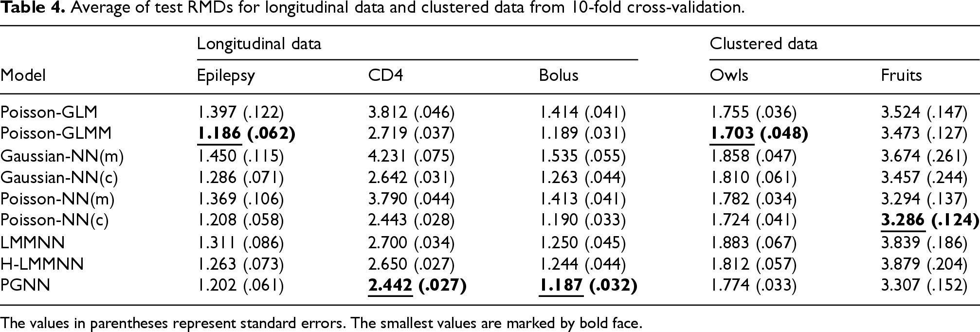
Average of test RMDs for longitudinal data and clustered data from 10-fold cross-validation.

	Longitudinal data			Clustered data
Model	Epilepsy	CD4	Bolus	Owls	Fruits
Poisson-GLM	1.397 (.122)	3.812 (.046)	1.414 (.041)	1.755 (.036)	3.524 (.147)
Poisson-GLMM	1.186 (.062)	2.719 (.037)	1.189 (.031)	1.703 (.048)	3.473 (.127)
Gaussian-NN(m)	1.450 (.115)	4.231 (.075)	1.535 (.055)	1.858 (.047)	3.674 (.261)
Gaussian-NN(c)	1.286 (.071)	2.642 (.031)	1.263 (.044)	1.810 (.061)	3.457 (.244)
Poisson-NN(m)	1.369 (.106)	3.790 (.044)	1.413 (.041)	1.782 (.034)	3.294 (.137)
Poisson-NN(c)	1.208 (.058)	2.443 (.028)	1.190 (.033)	1.724 (.041)	3.286 (.124)
LMMNN	1.311 (.086)	2.700 (.034)	1.250 (.045)	1.883 (.067)	3.839 (.186)
H-LMMNN	1.263 (.073)	2.650 (.027)	1.244 (.044)	1.812 (.057)	3.879 (.204)
PGNN	1.202 (.061)	2.442 (.027)	1.187 (.032)	1.774 (.033)	3.307 (.152)

The values in parentheses represent standard errors. The smallest values are marked by bold face.

Tables 3 and 4 present the average test RMSPEs and RMDs for both longitudinal and clustered datasets. Computing times and confidence intervals are reported in Appendix B. In terms of RMSPE and RMD, PGNN achieved the best performance in most cases (5 times) except for the owls data, followed by GLMM (3 times) and Poisson-NN(c) (2 times). For datasets with limited sample sizes or approximately linear underlying structures, such as the Epilepsy data, classical GLMMs may remain competitive or even preferable in terms of both predictive accuracy and computational efficiency. Lee et al.¹³ highlighted the importance of employing heavy-tailed random effects models with additional dispersion models (e.g. double HGLMs), suggesting that further extensions of neural network-based approaches to incorporate dispersion modeling may offer substantial benefits in capturing such complex characteristics. While neural networks are widely recognized for improving prediction performance in independent datasets, our results indicate that incorporating subject-specific random effects is often necessary for neural networks to achieve improved prediction accuracy in correlated datasets with high-cardinality categorical features.

7. Discussion

When the data contains high-cardinality categorical features, introducing random effects into neural networks is advantageous. We develop a subject-specific PGNN for clustered count data using the new h-likelihood. The h-likelihood enables an end-to-end learning algorithm using the single objective function. By introducing subject-specific random effects, neural networks can effectively identify the nonlinear effects of the input variables. Section 3.2 demonstrates that the proposed estimating equations remain unbiased under $E (u_{i}) = 1$ , even when the random effects distribution is misspecified. Simulation studies in Section 5.3 show that the prediction performance of the PGNN remains competitive under various misspecified random effects distributions.

Section 5.4 illustrates that the proposed framework can be extended to structured correlated random effects. However, extending the PGNN to accommodate multiple random effects with more complex or hierarchical correlation structures remains an open challenge. While enhanced Laplace approximations³⁹ provide a potential avenue for modeling temporal and spatially correlated random effects,⁴⁰ their application in conjunction with stochastic optimization is computationally demanding, even for relatively simple GLMM settings. Uncertainty quantification and predictive interval construction in neural network models with random effects also remain challenging and are beyond the scope of the present work, but constitute important directions for future research.

Various state-of-the-art network architectures can be readily incorporated into the h-likelihood framework, as demonstrated through the feature-selection example based on multi-head attention. With the growing interest in integrating deep learning models with statistical models, further exploration of random effects in neural networks for improved interpretability represents another promising avenue for future research.

Footnotes

ORCID iDs

Hangbin Lee

Il Do Ha

Changha Hwang

Youngjo Lee

Funding

This research was supported by the National Research Foundation of Korea (NRF) grant funded by the Korea government (MSIT) (RS-2026-25477861, RS-2023-00240794, RS-2022-NR068754).

Declaration of conflicting interests

The authors declared no potential conflicts of interest with respect to the research, authorship, and/or publication of this article.

A technical details

B Detailed results of simulation studies and real data analyses

This section presents detailed results of simulation studies in Section 5 and real data analyses in Section 6. Table 5 shows the computation times for simulation studies. Tables 6 and 7 show the confidence intervals of RMSPEs and RMDs for real data analyses, respectively. Table 8 shows the computation times for real data analyses.

C Additional simulation studies

References

LeCun

Bengio

Hinton

. Deep learning. Nature 2015; 521: 436–444.

Goodfellow

Bengio

Courville

. Deep learning. Cambridge, MA: MIT press, 2016.

Lee

Nelder

. Hierarchical generalized linear models. J R Stat Soc: Ser B (Methodol) 1996; 58: 619–656.

Nelder

Wedderburn

. Generalized linear models. J R Stat Soc Ser A: Stat Soc 1972; 135: 370–384.

Simchoni

Rosset

. Using random effects to account for high-cardinality categorical features and repeated measures in deep neural networks. Adv Neural Inf Process Syst 2021; 34: 25111–25122.

Simchoni

Rosset

. Integrating random effects in deep neural networks. J Mach Learn Res 2023; 24: 1–57.

Lee

. H-likelihood approach to deep neural networks with temporal–spatial random effects for high-cardinality categorical features. In: International conference on machine learning, 2023, pp.18974–18987.

Tran

Nguyen

Nott

, et al. Bayesian deep net GLM and GLMM. J Comput Graph Stat 2020; 29: 97–113.

Bishop

Nasrabadi

. Pattern recognition and machine learning. Vol. 4. New York, NY: Springer, 2006.

10.

Blei

Kucukelbir

McAuliffe

. Variational inference: a review for statisticians. J Am Stat Assoc 2017; 112: 859–877.

11.

Mandel

Ghosh

Barnett

. Neural networks for clustered and longitudinal data using mixed effects models. Biometrics 2023; 79: 711–721.

12.

Breslow

Clayton

. Approximate inference in generalized linear mixed models. J Am Stat Assoc 1993; 88: 9–25.

13.

Lee

Nelder

Pawitan

. Generalized linear models with random effects: unified analysis via H-likelihood. 2nd ed. Boca Raton, FL: Chapman and Hall/CRC, 2017.

14.

Heagerty

Zeger

. Marginalized multilevel models and likelihood inference (with comments and a rejoinder by the authors). Stat Sci 2000; 15: 1–26.

15.

Lee

Nelder

. Hierarchical generalised linear models: a synthesis of generalised linear models, random-effect models and structured dispersions. Biometrika 2001; 88: 987–1006.

16.

Roulin

Bersier

. Nestling barn owls beg more intensely in the presence of their mother than in the presence of their father. Anim Behav 2007; 74: 1099–1106.

17.

Henderson

Shimakura

. A serially correlated gamma frailty model for longitudinal count data. Biometrika 2003; 90: 355–366.

18.

Thall

Vail

. Some covariance models for longitudinal count data with overdispersion. Biometrics 1990; 46: 657–671.

19.

Henry

Erice

Tierney

, et al. A randomized, controlled, double-blind study comparing the survival benefit of four different reverse transcriptase inhibitor therapies (three-drug, two-drug, and alternating drug) for the treatment of advanced aids. J Acquir Immune Defic Syndr Hum Retrovirol 1998; 19: 339–349.

20.

Rodrigo

Tsokos

. Bayesian modelling of nonlinear Poisson regression with artificial neural networks. J Appl Stat 2020; 47: 757–774.

21.

Henderson

Kempthorne

Searle

, et al. The estimation of environmental and genetic trends from records subject to culling. Biometrics 1959; 15: 192–218.

22.

Gilmour

Anderson

Rae

. The analysis of binomial data by a generalized linear mixed model. Biometrika 1985; 72: 593–599.

23.

Harville

Mee

. A mixed-model procedure for analyzing ordered categorical data. Biometrics 1984; 40: 393–408.

24.

Schall

. Estimation in generalized linear models with random effects. Biometrika 1991; 78: 719–727.

25.

Wolfinger

. Laplace’s approximation for nonlinear mixed models. Biometrika 1993; 80: 791–795.

26.

Lee

Nelder

. Conditional and marginal models: another view. Stat Sci 2004; 19: 219–238.

27.

Dauphin

Pascanu

Gulcehre

, et al. Identifying and attacking the saddle point problem in high-dimensional non-convex optimization. Adv Neural Inf Process Syst 2014; 27: 1–9.

28.

Loshchilov

Hutter

. Sgdr: stochastic gradient descent with warm restarts. arXiv preprint arXiv:160803983, 2016.

29.

Lee

. Comparison of hierarchical likelihood versus orthodox best linear unbiased predictor approaches for frailty models. Biometrika 2005; 92: 717–723.

30.

Chollet

, et al. Keras. https://keras.io, 2015.

31.

Abadi

Agarwal

Barham

, et al. TensorFlow: large-scale machine learning on heterogeneous systems. http://tensorflow.org, 2015.

32.

Paszke

Gross

Massa

, et al. Pytorch: an imperative style, high-performance deep learning library. In: Advances in neural information processing systems 32, 2019, pp.8024–8035. Curran Associates, Inc.

33.

Venables

Ripley

. Modern applied statistics with S. 4th ed. New York: Springer, 2002.

34.

Maruo

Ishii

Yamaguchi

, et al. bcmixed: a package for median inference on longitudinal data with the Box–Cox transformation. R J 2021; 13: 253–265.

35.

Gonçalves

Cabral

. cold: an R package for the analysis of count longitudinal data. J Stat Softw 2021; 99: 1–34.

36.

Brooks

Kristensen

van Benthem

, et al. glmmTMB balances speed and flexibility among packages for zero-inflated generalized linear mixed modeling. R J 2017; 9: 378–400.

37.

Banta

Stevens

Pigliucci

. A comprehensive test of the ‘limiting resources’ framework applied to plant tolerance to apical meristem damage. Oikos 2010; 119: 359–369.

38.

Bates

Mächler

Bolker

, et al. Fitting linear mixed-effects models using lme4. J Stat Softw 2015; 67: 1–48.

39.

Han

Lee

. Enhanced Laplace approximation. J Multivar Anal 2024; 202: 105321.

40.

Lee

. On the statistical foundations of h-likelihood for unobserved random variables. arXiv preprint arXiv:231009955, 2024.

41.

Breiman

. Random forests. Mach Learn 2001; 45: 5–32.

42.

Martins

Astudillo

. From softmax to sparsemax: a sparse model of attention and multi-label classification. In: International conference on machine learning, 2016, pp.1614–1623, PMLR.

43.

Škrlj

Džeroski

Lavrač

, et al. Feature importance estimation with self-attention networks. arXiv preprint arXiv:200204464, 2020.

44.

Arik

SÖ

Pfister

. Tabnet: attentive interpretable tabular learning. Proc AAAI Conf Artif Intell 2021; 35: 6679–6687.