
Abstract
The measurement of individual differences in specific cognitive functions has been an important area of study for decades. Often the goal of such studies is to determine whether there are cognitive deficits or enhancements associated with, for example, a specific population, psychological disorder, health status, or age group. The inherent difficulty, however, is that most cognitive functions are not directly observable, so researchers rely on indirect measures to infer an individual’s functioning. One of the most common approaches is to use a task that is designed to tap into a specific function and to use behavioral measures, such as reaction times (RTs), to assess performance on that task. Although this approach is widespread, it unfortunately is subject to a problem of reverse inference: Differences in a given cognitive function can be manifest as differences in RTs, but that does not guarantee that differences in RTs imply differences in that cognitive function. We illustrate this inference problem with data from a study on aging and lexical processing, highlighting how RTs can lead to erroneous conclusions about processing. Then we discuss how employing choice-RT models to analyze data can improve inference and highlight practical approaches to improving the models and incorporating them into one’s analysis pipeline.
Researchers in psychology and related fields have long been interested in identifying whether specific cognitive functions differ across individuals. They might investigate if people with depression show a deficit in memory (Brand et al., 1992), or if children’s implicit learning is similar to adults’ (Meulemans et al., 1998), or if people with stronger inhibitory control show greater functional MRI activation in a specific neural region (Congdon et al., 2010). Such investigations are a core component of the National Institutes of Mental Health’s Research Domain Criteria (RDoC) initiative, which is aimed at identifying dimensions of cognitive functioning associated with abnormal and normal behavior (Insel et al., 2010). Thus, the degree to which individual differences in cognitive function can be successfully measured has strong implications for a wide range of scientific disciplines, from clinical psychology to health science.
Accordingly, it is critical that studies of cognitive function provide valid measures of the functions of interest. The primary challenge is that most, if not all, cognitive functions are not directly observable. One cannot “see” a person’s level of attentional control; instead, one must rely on indirect measures, such as reaction times (RTs) or error rates in an attention task. Although such measures have been useful, our concern is that measures of cognitive processes do not always measure what they are supposed to measure. In this article, we provide an overview of this measurement problem with an example from published data and then discuss how incorporating cognitive modeling into the analysis pipeline can mitigate the issue. We close with discussion of how to best adopt model-based analyses and how to encourage and improve their usage in the future.
The Reverse-Inference Problem for RT Tasks
A common approach to measuring differences in cognitive function is to take a task designed to rely on a given function and then infer processing on the basis of behavioral performance. In the lexical decision task, for example, participants decide if strings of letters are words or not, and performance is typically measured by RTs. In general, such tasks are based on a simple forward inference (Fig. 1, top left): If a person has poor lexical processing, then that person will have slow RTs in the task. For most cognitive tasks, this forward inference is supported. For instance, lexical decision RTs are slower for low-frequency (uncommon) words compared with high-frequency (common) words (Rubenstein et al., 1970), and slower for visually degraded words compared with clearly presented ones (Yap et al., 2013). Thus, the cause, weaker lexical processing, does indeed lead to the effect, slower RTs.
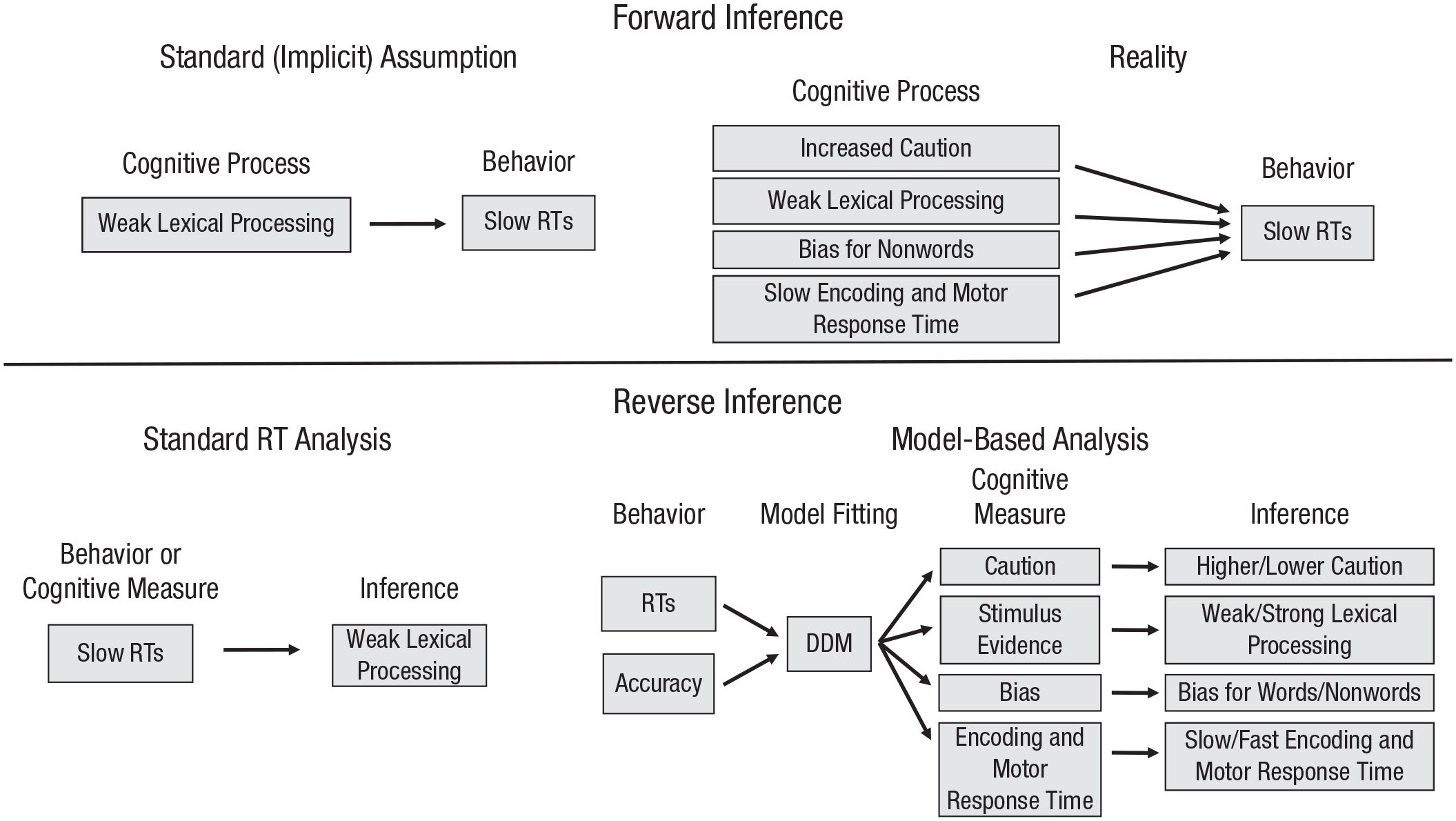
Illustration of forward (top) and reverse (bottom) inference for the lexical decision task. “Bias for nonwords” refers to a relative preference for the “nonword” response over the “word” response. “Stimulus evidence” refers to the task-relevant information, in this case, the lexicality of the letter string. DDM = drift diffusion model; RT = reaction time.
However, when one analyzes data from cognitive tasks, one is actually reversing the inference (Fig. 1, bottom left). The reverse-inference problem is a challenge for all scientific domains, arising when one observes an effect and infers that it resulted from a specific cause out of several possible causes. In this example, one infers that slower RTs indicate a person has weaker lexical processing, assuming that the slow RTs are a valid measure of the cognitive function of interest. Researchers have become so accustomed to this type of reverse inference that they substitute the phrase “weak lexical processing” for “slow RTs in the lexical decision task,” as if the two phrases are completely interchangeable. But such a reverse inference is valid only if the process of interest is the only factor that influences RTs.
Unfortunately, this is not always the case. As illustrated in Figure 1 (top right), RTs are also affected by differences in response caution (speed-vs.-accuracy preferences), response bias, and even the speed of encoding the stimulus and the motor response. Thus, a difference in RTs on a lexical decision task might reflect lexical processing, as the reverse inference assumes, but it might reflect other factors, such as caution or bias. Behavioral measures such as RTs and accuracy do not indicate which inference is correct. One way to reduce this reverse-inference problem is to model RT and accuracy data with choice-RT models (described in the next section), which decompose the behavioral data into separate measures of different decision components (Fig. 1, bottom right). This allows better determination of which factor is driving the difference in behavior.
To illustrate this issue, we take data from a study of aging and lexical decision (Ratcliff, Thapar, et al., 2004, Experiment 1) that compared lexical processing among older (65+) adults and college-age students. We have replotted the main summary data in Figure 2 (top), which shows two results: Older adults were slower than college students, and they had a larger word-frequency effect (i.e., a greater difference in RTs between high- and low-frequency words). Thus, the RT data support the inference that aging impairs the ability to access words in the lexicon, and that it has a particularly strong effect for words that are not commonly used.
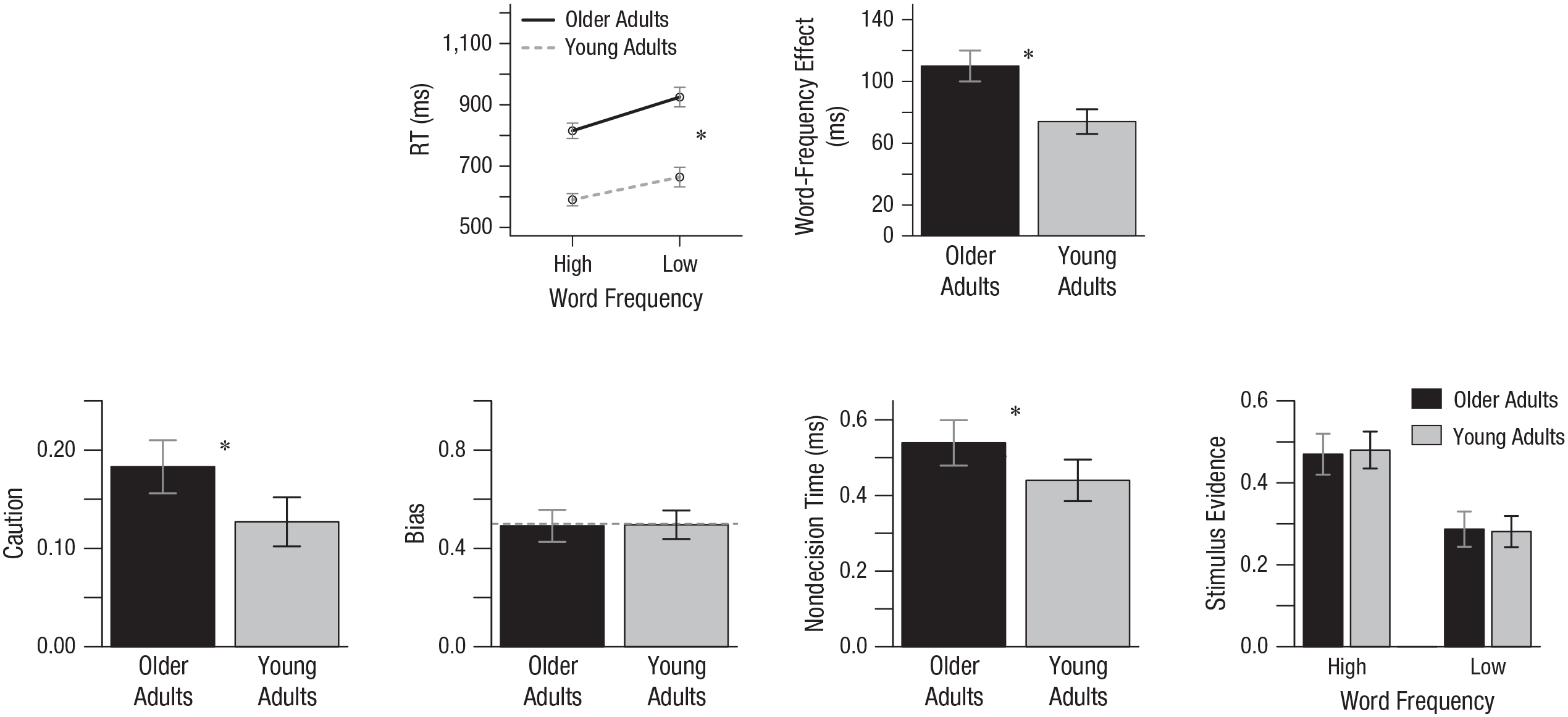
Results from the lexical decision task (Ratcliff, Thapar, et al., 2004, Experiment 1). The top panel shows mean reaction times (RTs) for high- and low-frequency words (left) and the difference between RTs for high- and low-frequency words (right), separately for older and young adults. The bottom panel shows the parameters for older and young adults’ caution, bias, nondecision time (time for encoding the stimulus and executing the response), and stimulus evidence (lexical processing) from the drift diffusion model that best fit the data. Error bars represent approximately 2 SEM. Asterisks indicate a significant difference between old and young participants (p < .05).
Although this conclusion might seem reasonable, it is valid only to the extent that the RTs are reflecting differences in lexical processing and nothing else. However, as Ratcliff, Thapar, et al. (2004) found, an RT model analysis of the data (Fig. 2 bottom) suggests a different conclusion: The older adults were more cautious and slower to press the response button than the college students (and thus their RTs were slower), but their lexical-processing ability was the same as the college students’. The inference changes significantly with the model-based analysis: Whereas the RT comparison suggests a deficit in lexical processing for older participants (especially for low-frequency words), the model-based analysis suggests that the older participants were simply more cautious and slower to make the motor response.
The reverse-inference problem inherent in the standard analysis of RTs (or error rates) creates a potentially misleading interpretation. This issue has wide-reaching implications for studies of individual and group differences, as different groups, such as people with and without depression or children with and without attention-deficit/hyperactivity disorder (ADHD), might have different levels of response caution, encoding and motor speed, or response bias. Fortunately, one can mitigate this issue by incorporating RT modeling into analyses, an approach we explore in the next section.
RT Models for Analyzing Data From Choice Tasks
Many, if not most, RT tasks are decision-making tasks. In lexical decision tasks, participants decide if the letter string is a word or not; in recognition memory tasks, they decide if a word was previously studied or not; and so on. Thus, RT and accuracy data from a lexical decision task are the result of both lexical processing and decision making. To obtain a cleaner measure of lexical processing, one needs to identify and separate out the effects of the decision process.
An increasingly common way to accomplish this is to analyze the data with decision models, such as the drift diffusion model (DDM; Ratcliff, 1978) or the linear ballistic accumulator (LBA) model (Brown & Heathcote, 2008). These models assume that the decision process involves the noisy accumulation of evidence until a criterion amount is reached. Decision behavior is driven by four primary components: response caution (speed-vs.-accuracy settings), response bias (leaning toward one response over the other), nondecision duration (amount of time needed for encoding the stimulus and executing the response), and stimulus evidence (a reflection of the ability to process the stimulus and extract accurate evidence for the correct response). In most cases, the stimulus-evidence component, termed the drift rate, is the one that actually reflects the task-specific process of interest (e.g., in a lexical decision task, the drift rate is driven by lexical processing). (For detailed explorations of these models, see the Recommended Reading.)
These models are instantiated mathematically and specify (mostly) precise relationships between potential causes (decision components) and effects (RTs and accuracy). Researchers can fit the model to behavioral data from a participant or condition, using a search algorithm that estimates the value of each component that most closely matches the observed data. The resulting set of parameter values allow researchers to compare separate measures of caution, bias, stimulus evidence, and nondecision time. These parameter values can be analyzed in the same manner as RTs—entered into t tests or analyses of variance, or used as regressors for functional MRI analyses, and so on.
Advantages of RT models
There are three primary advantages to employing model-based analyses. First, the models incorporate all of the behavioral data, including the proportion of correct responses (accuracy) and the RT distributions for both correct and error responses. Oftentimes, researchers will analyze RTs while more or less ignoring accuracy (or vice versa). Further, comparing individuals’ or groups’ mean RTs for correct responses neglects information from RTs for error responses and the shape of the RT distributions. RT distribution analyses, such as ex-Gaussian analyses (Heathcote et al., 1991), are an improvement in this regard, though they still do not account for accuracy or error RTs the way RT models do. In general, the relationship between accuracy and the RT distributions for correct and error responses provides critical information for understanding decision behavior. For example, DDM and LBA analyses typically show that faster error RTs than correct RTs for one response option indicate the presence of a response bias for the opposing response option (see White & Poldrack, 2014).
The second advantage is that RT models provide better specificity for identifying which factors are driving group or condition differences. For example, in the go/no-go task of inhibitory control, participants are asked to quickly respond (“go”) to a frequent stimulus but inhibit their response (“no go”) to an infrequent stimulus. Children with ADHD commonly show faster “go” RTs when trials are presented more rapidly, which was initially thought to reflect a deficit in task engagement. However, a diffusion-model analysis showed that faster presentation rates actually increased task engagement in these children, but also led to slower accumulation of “no-go” evidence that counteracted the higher engagement (Huang-Pollock et al., 2017). The modeling captured this effect through the relationships among accuracy, correct (go) RTs, and error (no-go) RTs, and countered the widespread belief that a fast presentation rate produces a deficit in arousal regulation for children with ADHD.
In a similar vein, a diffusion-model analysis changed the interpretation of feedback-learning performance in patients with schizophrenia (Moustafa et al., 2015). The behavioral data showed that these patients were significantly slower than control individuals on the learning task, but only slightly, nonsignificantly less accurate. The inference based on the standard accuracy metric would be that patients with schizophrenia were not significantly worse at learning from feedback. However, a DDM analysis of the data showed that they were significantly more cautious than control individuals and did show a deficit in punishment-based feedback learning. This learning deficit, which reduced accuracy, was offset by increased caution, which increased accuracy, and was apparent only once the model-based analysis identified and controlled for the specific effect of caution.
The third advantage of model-based analyses is that they can provide better sensitivity to small differences in processing. Individual differences in extraneous factors such as caution or bias add noise to the RT and accuracy measures, which can reduce researchers’ ability to detect small or weak differences. But this noise is controlled for with model-based analyses, as the effects of caution and bias are separated out from the effects of stimulus processing, which provides a cleaner measure of the latter. Multiple studies, including the schizophrenia study just mentioned, have found that the model-based measures show larger effect sizes than RTs and accuracy do, and in some cases, this increased sensitivity is enough to tip the balance from a null to a significant effect. For example, empirical studies have found that people with high anxiety show enhanced processing of threatening information when there are two or more stimuli competing for attention, but not when single stimuli are presented. This suggests that the threat bias is driven by the process of allocating attention between competing stimuli. In one such study (White et al. 2010), although a standard RT comparison showed a small, nonsignificant threat bias for singular stimuli in lexical decision, a DDM analysis of the data, which increased sensitivity by controlling for differences in caution and bias, showed a consistent, significant threat bias for high-anxiety participants. This model-based analysis suggests that the threat bias is still present when there are not multiple stimuli competing for attention; it is just smaller and harder to detect. The increased sensitivity offered by model-based analyses relative to standard RT models can be critical in domains such as clinical psychology, where effects are often small.
Using RT models to analyze data
Given the advantages of utilizing all the data and increasing specificity and sensitivity, we recommend that researchers apply models such as the DDM or LBA model to analyze their RT data. In many cases, the models can be added to the analysis pipeline with minimal extra effort, and they can often be used on data that have already been collected. To date, these models have been successfully applied to a wide range of tasks, including those that measure recognition memory (Ratcliff, Thapar, & McKoon, 2004), threat classification (White et al., 2016), inhibitory control (Gomez et al., 2007), and economic choice (Clithero, 2018). Likewise, these models have been used with functional MRI and electromyogram data (see Recommended Reading for sources providing further information).
There are a number of software packages available to ease the implementation of these models, including packages for MATLAB (Vandekerckhove & Tuerlinckx, 2008) and R Studio (Brown & Heathcote, 2008; Wagenmakers et al., 2007), as well as stand-alone packages (Singmann et al., 2022; Voss & Voss, 2007; Wiecki et al., 2013). For each of these packages, the researcher need only prepare the data according to the instructions and run the program. The output provides, for each participant or condition, a list of parameter estimates that reflect the levels of caution, bias, nondecision time, and stimulus evidence (task performance) and can then be used in the same manner as RTs for t tests, regressions, and other analyses.
Although the statistical packages increase usability, they also make it easier for one to potentially misuse the models when they are not appropriate. There are important considerations that ensure the models are providing valid parameter estimates, including having enough observations (usually 30+ per condition) and making sure that the model predictions match the observed data. A researcher who uses a model but does not verify its accuracy could end up with erroneous inferences. One simple way to avoid these pitfalls is to collaborate with researchers who have experience using these models; the experts can help to troubleshoot the process and leverage their experience when adjustments need to be made to the modeling process.
Limitations and future directions
Although using RT models to analyze data is a step in the right direction, it is not without limitations. First, the model-fitting process is simply a transformation of the data, and there are small correlations among the parameters that mean the estimates are not completely precise or unbiased (Ratcliff & Tuerlinckx, 2002). Thus, model-based analyses are still subject to the reverse-inference problem, albeit to a lesser degree than mean RTs or error rates. Second, the models perform best when there are a large number of trials and error RTs, which might not occur because of practical constraints and the nature of the tasks. Although these are structural problems that cannot be completely avoided, newer estimation approaches, including hierarchical Bayesian versions of the models, have been developed to improve application to sparse data (Alexandrowicz & Gula, 2020; Wiecki et al., 2013).
Future research can focus on extending RT models so that they incorporate task-specific processes and can be applied to new paradigms. For example, Lerche and Voss (2019) showed that the DDM can be used even when the decisions are slower than is typical (> 3 s, Lerche & Voss, 2019). Holmes et al. (2016) developed an LBA model in which the evidence can change over the course of the decision. And hybrid RT models that add components to describe where the decision evidence comes from can be developed. Although the DDM can be applied to lexical decision data, it says nothing about how lexical processing works. Hybrid models address this by adding a “front end” to describe how the stimulus is processed to provide the decision evidence. This evidence is fed into the “back end” of the decision process. For example, conflict paradigms such as the flanker task produce data patterns indicative of time-varying decision evidence, and these data cannot be captured by a standard DDM or an LBA model. But conflict-diffusion models that add conflict-control processes such as delayed suppression can successfully account for data from these tasks (Hubner et al., 2010; Ulrich et al., 2015; White et al., 2011).
Such model extensions (a) provide a formal framework for testing theoretical assumptions, (b) expand the tasks to which the models can be applied, and (c) add constraints to improve parameter identifiability (i.e., identifying which parameter values are estimated accurately). However, these newer hybrid models need to be validated, particularly if they are to be used to analyze RT data. For instance, a recent study (White et al., 2018) found that conflict-diffusion models had significant parameter trade-offs (i.e., changes in one parameter could be compensated for by changes in another). These trade-offs made the raw parameter values difficult to estimate accurately, but a targeted combination of specific parameters improved their validity.
Conclusion
Psychologists should look toward improving the way they measure cognitive functions, particularly when RT tasks are used to assess individual differences. Although RT-based measures have provided important insights over the past 100+ years, they are still noisy and prone to problems of reverse inference. It is important to remember that in a task like lexical decision, the RTs are a proxy for lexical processing, not a perfect measure of it. Analysis with choice-RT models can reduce the reverse-inference problem by incorporating all of the data, providing better specificity for which cognitive components differ among individuals and better sensitivity for detecting small differences.
We recommend that, when feasible, researchers add model-based analyses to their pipeline for RT data. Often this can be done without much overhead, particularly when collaborations are formed with experienced modelers. Meaningful progress in psychology cannot occur if researchers are not measuring what they think they are measuring, and cognitive modeling provides one approach to improve inferences about cognitive functions.
Recommended Reading
Donkin, C., Brown, S., & Heathcote, A. (2011). Drawing conclusions from choice response time models: A tutorial using the linear ballistic accumulator. Journal of Mathematical Psychology, 55(2), 140–151. https://doi.org/10.1016/j.jmp.2010.10.001. A tutorial focusing on how to use and interpret results from a reaction time (RT) model, with a worked example illustrating the general principles for employing such models and drawing appropriate inferences from the results.
Forstmann, B. U., Ratcliff, R., & Wagenmakers, E.-J. (2016). Sequential sampling models in cognitive neuroscience: Advantages, applications, and extensions. Annual Review of Psychology, 67, 641–666. https://doi.org/10.1146/annurev-psych-122414-033645. An overview of how and why to use RT models in conjunction with neural data such as from functional MRI or electroencephalography, highlighting how the models can be used to bridge the neural recordings, behavioral responses, and underlying cognitive mechanisms.
Ratcliff, R., Smith, P. L., Brown, S. D., & McKoon, G. (2016). Diffusion decision model: Current issues and history. Trends in Cognitive Sciences, 20(4), 260–281. https://doi.org/10.1016/j.tics.2016.01.007. An overview of diffusion models with a focus on historical development, core aspects of the model framework, and current applications.
White, C. N., Ratcliff, R., Vasey, M. W., & McKoon, G. (2010). Using diffusion models to understand clinical disorders. Journal of Mathematical Psychology, 54(1), 39–52. https://doi.org/10.1016/j.jmp.2010.01.004. A discussion of how RT models can help improve understanding of cognitive processing in clinical populations, although the general approach can be applied to other populations (e.g., people with hypertension) and domains (e.g., developmental or social psychology).