Supply Chain Network Design Based on Integration of Forward and Reverse Logistics

Abstract

This article describes a mathematical model for the design of supply chain network for a company that sells its products through a set of retail stores that integrates both the movement of fresh products and the returns from the customers. Specifically, the company faces a situation where, given the location and demand from the set of retail stores, it wishes to decide where to locate the warehouses (or distribution centres) and test centres and the routes to be used in transporting the fresh products from warehouses to stores, returned products from stores to test centres and finally, re-stockable returned products from test centres to warehouses. This is formulated as a binary integer linear programming problem. The problem is solved using LINGO and then, an analysis is performed to determine the sensitivity of the optimal solution to different parameters, including sales volumes, return rates, costs of operation and transportation and the various prices.

Keywords

Supply chain design supply chain network reverse logistics facilities location ILP sensitivity analysis

Introduction

The performance of any supply chain at best is as good as its design. While the performance of a well-designed supply chain network may be better or worse depending on the operating decisions made, a poorly designed network will never be able to overcome the limitations of its inferior design and deliver superlative performance (Meepetchdee & Shah, 2007). Supply chain network design, in turn, depends on a host of factors, both internal to the company—like its choice of products, markets and competitive strategy, its cost structure emanating from its choice of technology and production and logistical processes and even its existing network—and external like the demand of its products and its geographical distribution, location of suppliers, tariffs, tax incentives, actions of competitors and perhaps, even disaster risks (Abe & Ye, 2013). As most of these factors are dynamic in their nature, supply chain designs need to be reviewed and modified whenever required, though not very frequently as, by its very nature, it is a strategic decision.

Supply chain network design includes determining the different types of facilities and their roles; location, number and capacities of each type of facility and the quantity of the flow between them (Amiri, 2006). It is a complex, strategic decision problem, often involving multiple and conflicting objectives such as profit (or cost), service level, responsiveness and so on. The importance of supply chain network design can be gauged from the large body of research work incorporating mathematical programming, simulation, multi-objective decision making, empirical studies and other methodologies, as well as the review papers like the ones by Akcali, Cetinkaya and Uster (2009), Carter and Ellram (1998), Fleischmann, Bloemhof-Ruwaard, Dekker, van der Laan, van Nunen and van Wassenhove (1997), Melo, Nickel and Saldanha-da-Gama (2009), Snyder (2006) and Srivastava (2007).

Supply chain networks are often designed considering only the forward logistics, wherein all processes involved in the movement of goods from suppliers through manufacturers, distributors and retailers to the end customers are analyzed. But in many supply chains, physical goods as well as their value do not get fully consumed once they reach the end customer. Coordination between the forward movement and the successive processes after the product return may be imperative to capture the value still present in the returned product/other associated resources. While liberal customer return policies may emphasize customer satisfaction (Lee et al., 2012), ‘…used products are sold on secondary markets, outdated products are upgraded to meet latest standards again, failed components are repaired to serve as spare parts, unsold (and returned) stock is salvaged, reusable packaging is returned and refilled, and used products are recycled into raw materials again’ (Wadhwa & Madaan, 2007) to enhance the value of the output produced by the supply chain. ‘Reverse logistics’ includes the new set of processes that aim at capturing economic as well as environmental values from the products/resources taken back from customer, thus broadening the scope and the span of supply chain networks.

The strategic importance of warehouse location and the design of the supply chain network is well recognized in most industries. In some of these industries, the return rate is also considerably high. A survey by the Reverse Logistics Executive Council found that in the United States (US), return rates varied significantly across industries and for many industries, it was vital to manage the reverse flow (Rogers & Tibben-Lembke, 1999). The return rates were as high as 50 per cent for magazine publishing, 20–30 per cent for book publishing and greeting cards and 10–20 per cent for computer manufacturers.

This article is organized in seven sections. After this brief introduction, we carry out a review of literature on integrated forward and reverse logistics network design in the second section. In the third section, we formally define the problem and the assumptions made. The mathematical formulation of the problem is presented in the fourth section where we formulate the decision problem as an integer linear programming (ILP) problem. We next present a small application and its solution in the fifth section. The sixth section discusses the solution and its sensitivity to some of the key parameters. Finally, in the last section, we present conclusion and the limitations of our model.

Review of Literature

An early usage of the term ‘reverse logistics’ is found in Stock (1992) in which, although the usage of the term in the context of waste disposal and management of hazardous materials is highlighted, the perspective is broadened to include ‘all issues relating to logistics activities carried out in source reduction, recycling, substitution, reuse of materials and disposal’. As the use of reverse logistics concept was found to be much broader than in the context of environmental management, the definitions were also gradually widened to include flows of new products returned for commercial reasons, returns of, say, packaging materials to manufacturers or to parties other than producers, including specialized recovery companies. Fleischmann (2000) defined reverse logistics as ‘the process of planning, implementing, and controlling the efficient, effective inbound flow and storage of secondary goods and related information opposite to the traditional supply chain direction for the purpose of recovering value or proper disposal’.

Rogers, Melamed and Lembke (2012) present an excellent review of published research on modelling and analysis of reverse logistics as well as a summary of modelling opportunities in this area. They mention that both analytical and simulation models have been used in the literature in all areas of reverse logistics, like reverse logistics network design, returned product route planning and scheduling, central return processing optimization, secondary market optimization and product disposition revenue maximization. An understanding of the various processes involved in the reverse logistics of a retailer is presented by Hsu, Alexander and Zhu (2009), while Stock and Mulki (2009) do the same for manufacturers, wholesalers/distributors and retailers.

Many authors have used facility location models based on mixed integer linear programming (MILP) for network designing and combinatorial optimization theory. Kroon and Vrijens (1995) discuss the design of an integrated network for reusable containers based on MILP. They address the role of different actors, the economics of the system, the cost allocation to the different actors, the amount of containers needed and the locations of the depots for the containers. Barros, Dekker and Scholten (1998) present a case study addressing the design of an integrated logistics network for recycling sand resulting from the processing of construction waste in the Netherlands. They develop a capacitated facility location model based on MILP in which they evaluate multiple scenarios and finally select the solution with the best worst-case behaviour. Jayaraman, Guide Jr and Srivastava (1999) present an analysis of logistics network based on mixed integer programming (MIP) of re-manufacturing facilities for electronic equipment. Similarly, Krikke, Kooi and Schurr (1999) develop a mixed integer programme to design an un-capacitated reverse logistics network. Louwers, Kip, Peeters, Souren and Flapper (1999) discuss a reverse open-loop network model with continuous potential locations using non-linear programming for carpet waste. Lieckens and Vandaele (2007) combine MILP with a queuing model to design a reverse logistics network.

Jayaraman, Patterson and Rolland (2003) discuss a model for reverse distribution network and solve it with a heuristic solution methodology. Min et al. (2006) proposes a deterministic model to design a reverse logistics network involving products returned due to either defects or changes in customers’ needs/preferences. Srivastava (2008) developed reverse logistics network design model based on maximizing profits for various scenarios in practical settings using a hierarchical optimization model.

Khajavi, Seyed-Hosseini and Makui (2011) develop an MIP-based model to optimize a multistage capacitated supply chain integrating both forward and reverse logistics. Ozceylan and Paksoy (2013) present an MIP model for a closed-loop supply chain network that includes both forward and reverse flows with multi-periods and multiple components. However, their model assumes known capacities for different facilities as well as disassembly and refurbishing as the only disposal of product returns.

Most authors have chosen to minimize cost as part of their formulation and only a few have formulated the problem to maximize profit. Tan and Kumar (2006) developed a system dynamic model to maximize profit from the reverse logistics operations of a computer manufacturer. Lee et al. (2012) supported the assertion of Guide et al. (2006) that maximization of profit is a better objective than minimization of cost and chose to maximize profit in their non-linear mixed integer programme formulation. Das (2012) also developed an MIP model that integrated the output from a recovery model into a new product model to achieve coordination between two separate markets of new products and recoverables. We have formulated the integrated forward and reverse logistics in our model as a binary ILP problem.

Problem Description and Assumptions

We consider a company that sells products like garments, or shoes or sports goods through its chain of retail stores all across India. Though there could be a large variety of products, these could be aggregated for transportation and storage purposes and the aggregated demand could be expressed in common units like kilogram (kg) or truckload. It supplies the retail stores from multiple warehouses (or distribution centres, DCs) through frequent deliveries. The company has an idea of the average sales volume (in aggregate units) per period and the average return rate at each of these stores. The company buys the products from manufacturers who deliver the products at the warehouses as specified by the company. We consider the supply chain from the warehouses onwards. It is possible that the company produces some of the products itself and is one of the manufacturers. All products returned by the customers (reverse logistics) are first collected at the retail stores and transported to a test centre at which their mode of disposal is decided and a fraction of the returned products, with some additional processing or packaging—if required—is then sent back to a warehouse for onward transmission to a retail store.

To begin with, only the locations of the retail stores are known. The company needs to decide the number and the locations of its warehouses and test centres. A warehouse will be used for storing and transporting products to retail stores, whereas a test centre will be used for testing the returned products. The supply chain network will also specify which warehouse or warehouses will meet the demand for each retail store, that is, the flow of products from warehouses to retail stores. Similarly, the design of the supply chain network must also specify the flow (of product returns) from retail stores to test centres as well as from test centres back to warehouses.

Further, the company has shortlisted some cities (and sites within the cities) for possible location of its warehouses. Similarly, it has also prepared a second shortlist of candidate locations for its test centres, some or many of which may be common to the first shortlist of locations for warehouses. Obviously, a common location for both warehouse and test centre may save on the transportation cost from the test centre to the warehouse, while it has also been found that ‘DCs do not work well managing both forward and reverse distribution at the same location’ (Rogers et al., 2012) as the returned product almost always gets a lower priority. Since we are designing the supply chain network, we are not assuming any capacity constraints, either for a warehouse or for a test centre. Rather the cost of operating a warehouse, as that of a test centre, is made dependent on the capacity required to handle the flow of products through it.

There are seven types of costs which affect the company’s decision in selecting the locations of its test centres and warehouses. These are:

Fixed cost of operating a warehouse.

Variable cost of operating a warehouse.

Fixed cost of operating a test centre.

Variable cost of operating a test centre.

Transportation cost of products from a warehouse to a retail store.

Transportation cost of product returns from a retail store to a test centre.

Transportation cost of re-stockable product returns from a test centre to a warehouse.

The company can reduce its transportation costs by operating more warehouses and test centres; but then its costs of operating the warehouses and the test centres would rise. This trade-off between transportation costs on one hand, and the operating costs (fixed and variable costs) on the other, would be important in the final design of the supply chain network. In fact, since we assume different procurement prices at each warehouse and different secondary price at each test centre, we formulate our decision problem as one of maximizing profit rather than one of minimizing cost.

Figure 1.

Source: Author’s own.

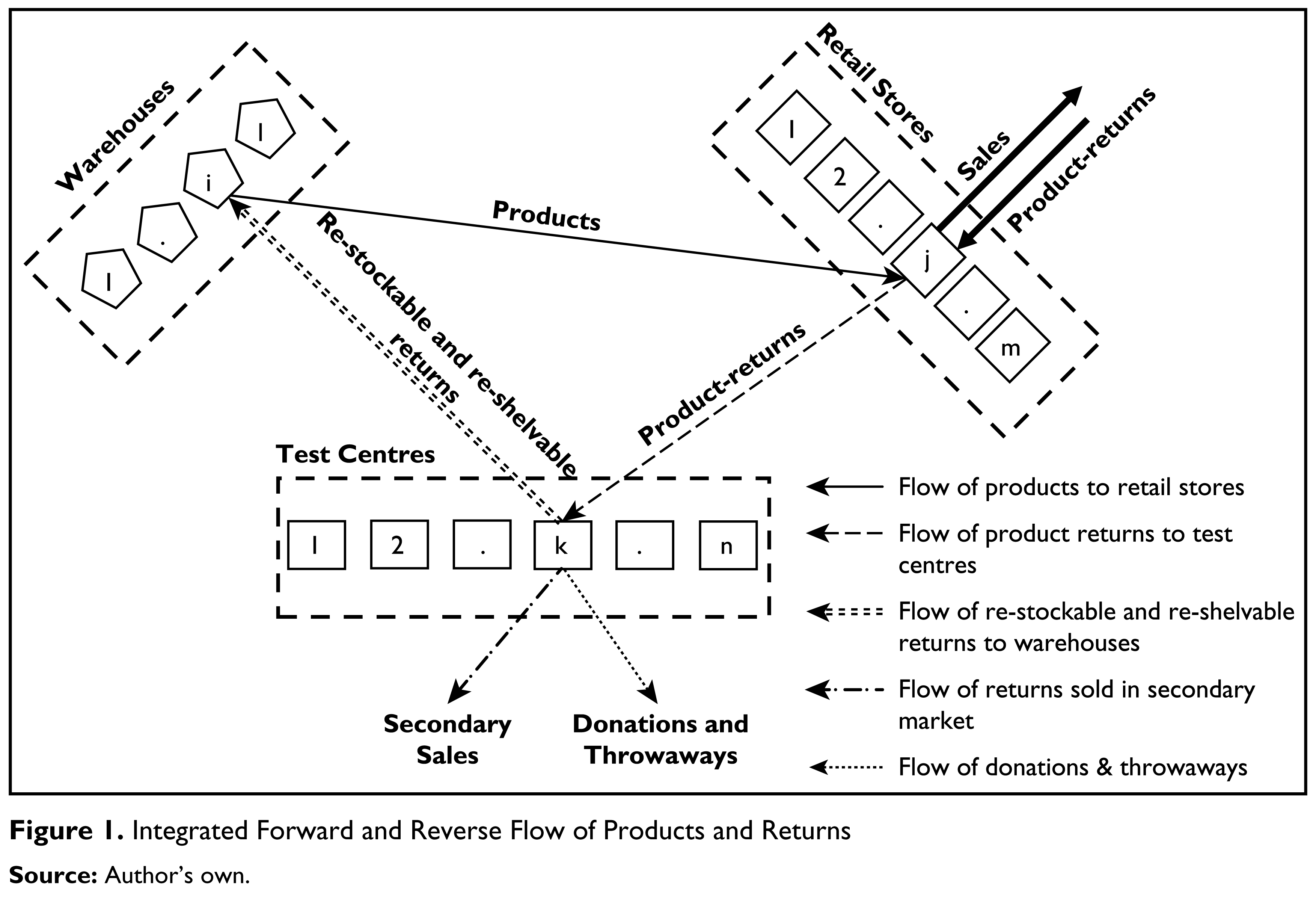
Figure 1 presents a diagrammatic representation of different flows in the supply chain network. In our design, each retail store will be fully served by a single warehouse. Similarly, each retail store will send back its product returns to a single test centre. We assume that products are returned by customers only at the retail stores. This is a realistic assumption because the customer would be inclined to return the products to the closest retail store to get a refund or to purchase another product. From the retail stores, returned products are taken to test centres. At a test centre, products are tested, and on the basis of the test results, the mode of disposal is decided. A particular returned product may be found to be fit for:

Re-stocking and re-shelving.

Reselling to secondary markets.

Donations.

Throwaway.

Returns segregated for re-stocking and re-shelving are sent to a warehouse after repackaging them, if necessary, while those identified for reselling to secondary markets are sold to the secondary sellers at the test centre itself. The company also donates and throws away the identified product returns from the test centre itself. So, we are not considering any transportation cost for reselling to secondary markets, nor are we considering any cost for donations and throwaways.

We know the average aggregate sales of the products and the average return rate in each retail store, unit transportation cost between a retail store and each of the candidate warehouse or test centre and between a test centre and a warehouse. We also know the fixed and the variable cost of operating each candidate warehouse and test centre. The supply chain network design will determine which candidate warehouse and which candidate test centre should be operated and the flows between the chosen warehouses, the test centres and the retail stores.

Model Formulation

We use the following parameters and variables for defining our formulation:

Parameters

i = Index of candidate sites for warehouses (or DCs) that would send products to retail stores.

l = Total number of candidate sites for warehouses.

j = Index of retail stores that sell products to customers.

m = Total number of retail stores.

k = Index of candidate sites for test centres that would test the product returns, decide the mode of disposal and send re-stockable returns to warehouses.

For the ith warehouse:

PP_i = Procurement price per unit of fresh products at the ith candidate warehouse site.

f ^WH_i = Fixed cost of operating the ith candidate warehouse site per period.

v^WH_i = Variable cost of operating the ith candidate warehouse site per unit per period.

For the jth retail store:

SP_j = Selling price per unit of fresh products at the jth retail store.

S_j = Sales of the product (in units and net of returns) at the jth retail store per period.

ρ_j = Total returns as a proportion of sales (in units) at the jth retail store.

For the kth test centre:

DP_k = Secondary market selling price (discounted price) of returned products per unit at the kth candidate test centre site.

f ^TC_k = Fixed cost of operating the kth candidate test centre site per period.

v^TC_k = Variable cost of operating the kth candidate test centre site per unit per period.

Other parameters and movement costs:

μ = Re-stockable returns as a proportion of total returns.

ν = Secondary saleable returns as a proportion of total returns.

C¹_ij = Transportation cost per unit of the product from the ith candidate warehouse site to the jth retail store.

C²_jk = Transportation cost per unit of total returns from the jth retail store to the kth candidate test centre site.

C³_ki = Transportation cost per unit of re-stockable returns from the kth candidate test centre site to the ith candidate warehouse site.

M = A large number.

λ = A small number greater than zero.

Decision Variables

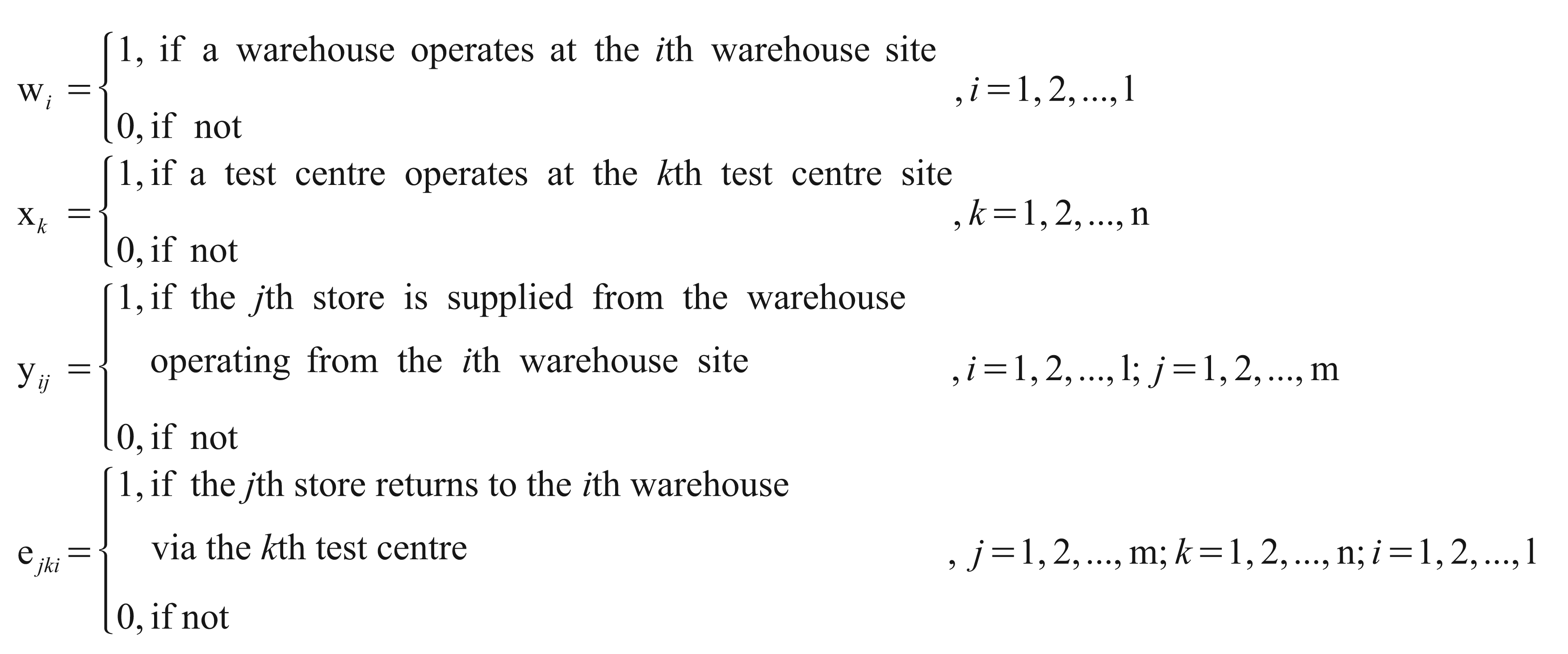
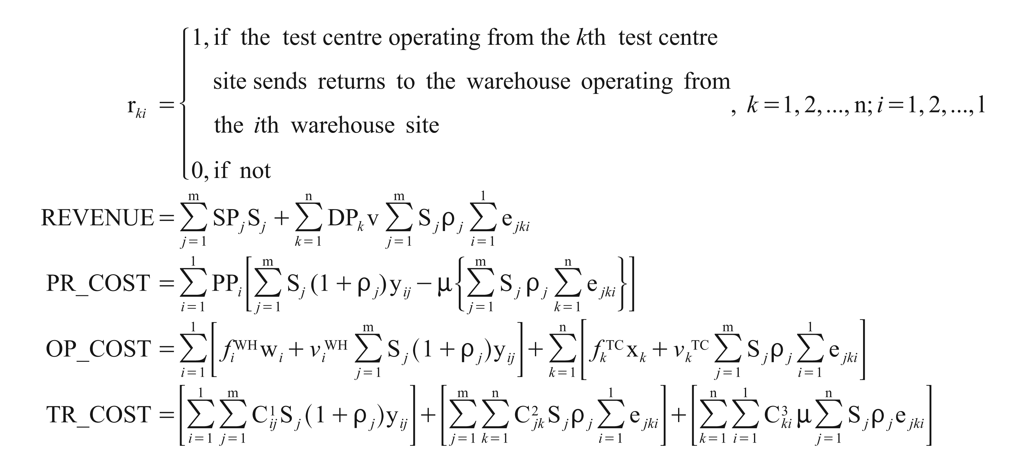
\begin{array}{l} w_{i} = {\begin{array}{l} 1, i f a w a r e h o u s e o p e r a t e s a t t h e i t h w a r e h o u s e s i t e \\ 0, i f n o t \end{array}, i = 1, 2, ..., l \\ x_{k} = {\begin{array}{l} 1, i f a t e s t c e n t r e o p e r a t e s a t t h e k t h t e s t c e n t r e s i t e \\ 0, i f n o t \end{array}, k = 1, 2, ..., n \\ y_{i j} = {\begin{array}{l} \begin{array}{l} 1, i f t h e j t h s t o r e i s \sup p l i e d f r o m t h e w a r e h o u s e o p e r a t i n g \\ f r o m t h e i t h w a r e h o u s e s i t e \end{array} \\ 0, i f n o t \end{array}, i = 1, 2, ..., l; j = 1, 2, ..., m \\ e_{j k i} = {\begin{array}{l} \begin{array}{l} 1, i f t h e j t h s t o r e r e t u r n s t o t h e i t h w a r e h o u s e \\ v i a t h e k t h t e s t c e n t r e \end{array} \\ 0, i f n o t \end{array}, j = 1, 2, ..., m; k = 1, 2, ..., n; i = 1, 2, ..., l \end{array}

Intermediate or Structural Variables

\begin{array}{l} r_{k i} = {\begin{array}{l} \begin{array}{l} 1, i f t h e t e s t c e n t r e o p t g f r o m t h e k t h t e s t c e n t r e \\ s i t e s e n d s r e t u r n s t o t h e w a r e h o u s e o p t g f r o m \end{array} \\ \begin{array}{l} t h e i t h w a r e h o u s e s i t e \\ 0, i f n o t \end{array} \end{array}, k = 1, 2, ..., n; i = 1, 2, ..., l \\ R E V E N U E = \sum_{j = 1}^{m} S P_{j} S_{j} + \sum_{k = 1}^{n} D P_{k} v \sum_{j = 1}^{m} S_{j} ρ_{j} \sum_{i = 1}^{1} e_{j k i} \\ P R_C O S T = \sum_{i = 1}^{1} P P_{i} [\sum_{j = 1}^{m} S_{j} (1 + ρ_{j}) y_{i j} - μ {\sum_{j = 1}^{m} S_{j} ρ_{j} \sum_{k = 1}^{n} e_{j k i}}] \\ O P_C O S T = \sum_{i = 1}^{1} [f_{i}^{W H} w_{i} + v_{i}^{W H} \sum_{j = 1}^{m} S_{j} (1 + ρ_{j}) y_{i j}] + \sum_{k = 1}^{n} [f_{k}^{T C} x_{k} + v_{k}^{T C} \sum_{j = 1}^{m} S_{j} ρ_{j} \sum_{i = 1}^{1} e_{j k i}] \\ T R_C O S T = [\sum_{i = 1}^{1} \sum_{j = 1}^{m} C_{i j}^{1} S_{j} (1 + ρ_{j}) y_{i j}] + [\sum_{j = 1}^{m} \sum_{k = 1}^{n} C_{j k}^{2} S_{j} ρ_{j} \sum_{i = 1}^{1} e_{j k i}] + [\sum_{k = 1}^{n} \sum_{i = 1}^{1} C_{k i}^{3} μ \sum_{j = 1}^{n} S_{j} ρ_{j} e_{j k i}] \end{array}

The Optimizing Model

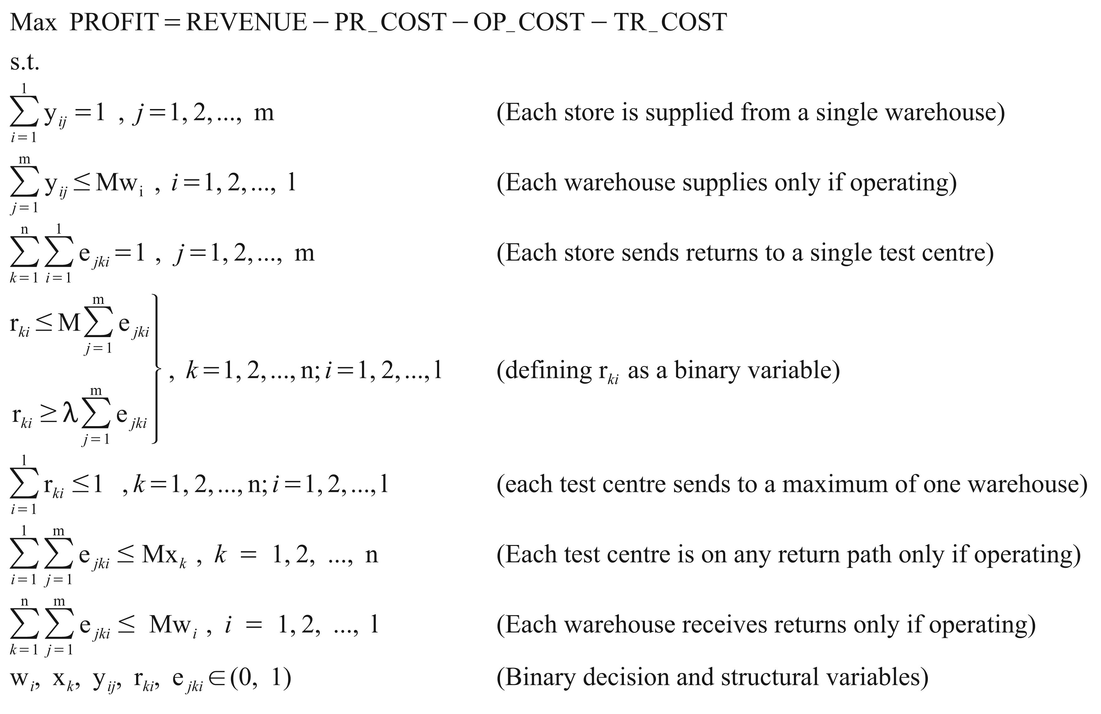
\begin{array}{l} M a x P R O F I T = R E V E N U E - P R_C O S T - O P_C O S T - T R_C O S T \\ \sum_{i = 1}^{1} y_{i j} = 1, j = 1, 2, ..., m (E a c h s t o r e i s \sup p l i e d f r o m a \sin g l e w a r e h o u s e) \\ \sum_{j = 1}^{m} y_{i j} \leq M w_{i}, i = 1, 2, ..., l (E a c h w a r e h o u s e \sup p l i e s o n l y i f o p e r a t i n g) \\ {\sum_{k = 1}^{n} \sum_{i = 1}^{1} e}_{j k i} = 1, j = 1, 2, ..., m (E a c h s t o r e s e n d s r e t u r n s t o a \sin g l e t e s t c e n t r e) \\ \begin{matrix} r_{k i} \leq M \sum_{j = 1}^{m} e_{j k i} \\ r_{k i} \geq λ \sum_{j = 1}^{m} e_{j k i} \end{matrix}}, k = 1, 2, ..., n; i = 1, 2, ..., l (d e f i n i n g r_{k i} a s a b i n a r y var i a b l e) \\ \sum_{i = 1}^{l} r_{k i} \leq 1, k = 1, 2, ..., n; i = 1, 2, ..., l (e a c h t e s t c e n t r e s e n d s t o a \max i m u m o f o n e w a r e h o u s e) \\ \sum_{i = 1}^{1} \sum_{j = 1}^{m} e_{j k i} \leq M x_{k}, k = 1, 2, ..., n (E a c h t e s t c e n t r e i s o n a n y r e t u r n p a t h o n l y i f o p e r a t i n g) \\ \sum_{k = 1}^{n} \sum_{j = 1}^{m} e_{j k i} \leq M w_{i}, i = 1, 2, ..., l (E a c h w a r e h o u s e r e c e i v e s r e t u r n s o n l y i f o p e r a t i n g) \\ w_{i}, x_{k}, y_{i j}, r_{k i}, e_{j k i} \in (0, 1) (B i n a r y d e c i s i o n a n d s t r u c t u r a l var i a b l e s) \end{array}

We have formulated the above integrated logistics problem as a binary ILP. The ILP maximizes the profit per period which is obtained by subtracting the total supply chain cost from the revenue per period. The revenue per period is from sale of products at the retail stores and from sale of returned products in the secondary market. Similarly, the supply chain cost per period is the sum of procurement cost, operating cost and the transportation cost per period.

The procurement cost of fresh products from manufacturers and vendors is for quantity net of re-stockable returns. The operating cost is the sum of the fixed and the variable cost of operating the warehouses and the test centres, respectively and the transportation cost is the sum of three transportation costs, namely, from warehouses to stores, from stores to test centres and from test centres to warehouses, respectively.

While y_ij and e_jki are binary decision variables representing whether the forward path from warehouse i to store j and from store j to warehouse i via test centre k are used or not, we have also introduced a binary structural variable r_ki to represent if test centre k should send product returns to warehouse i or not. This is required to represent the constraint that each test centre sends returns to a maximum of one warehouse. This constraint, as well as the ones representing that each store is supplied from a single warehouse and that each store sends returns to a single test centre are introduced from considerations of effectiveness and convenience, particularly because no capacity limitations have been assumed for any facility.

It may appear that we could use binary decision variables, p_jk and r_ki, to represent, respectively, if the route from the jth store to the kth test centre and the route from the kth test centre to the ith warehouse is used or not. However, this results in a quadratic objective function. By defining decision variables over the complete return path, e_jki, we could formulate this as a binary ILP, however at the cost of additional variables. This trade-off between a simpler objective function and fewer variables could be used differently in bigger problems. Of course, p_jk and r_ki values can always be obtained from the e_jki values by summing over the appropriate indices.

Application and Results

We apply the formulated problem to a smaller version of a realistic situation to demonstrate the appropriateness of the formulation as well as to interpret the results and study the sensitivity of the designed supply chain network to the parameters identified so that any conclusions derived therefrom can be used in designing as well as modifying similar supply chain networks.

In this application, we consider a company having 10 retail stores in different parts of the country selling the product. The stores get their supplies from warehouses (or DCs) and any returns from the customers are sent by the stores to test centres. The company has shortlisted six possible locations for the warehouses and another six candidate locations for test centres. Some of the candidate test centres are at the same locations as the candidate warehouse locations (three in number), while three additional locations are shortlisted only for possible test centre locations. In this conceptualization, we face a network facilities location problem where the nodes and the arcs are well defined. What is required is to choose some nodes and some arcs in such a way that the supply chain conditions for forward and backward logistics are satisfied and the profit per period is maximized. The parameters chosen for this problem are shown in the Appendix. When this problem is solved using LINGO, we find the solution as given in Table 1.

Table 1.

Optimal Solution—Forward and Return Paths

Supplied from WH	W-Dlh	W-Dlh	W-Dlh	W-Chn	W-Dlh	W-Dlh	W-Dlh	W-Dlh	W-Dlh	W-Dlh
	↓	↓	↓	↓	↓	↓	↓	↓	↓	↓
Store →	S-Ahd	S-Bgl	S-Bpl	S-Chn	S-Dlh	S-Hyd	S-Klk	S-Luc	S-Mum	S-Pun
	↓	↓	↓	↓	↓	↓	↓	↓	↓	↓
Sent to TC	T-Ahd	T-Hyd	T-Hyd	T-Hyd	T-Luc	T-Hyd	T-Luc	T-Luc	T-Ahd	T-Hyd
	↓	↓	↓	↓	↓	↓	↓	↓	↓	↓
And then to	W-Chn	W-Chn	W-Chn	W-Chn	W-Chn	W-Chn	W-Chn	W-Chn	W-Chn	W-Chn

Source: Author’s own.

Note: WH = warehouse; TC = test centre.

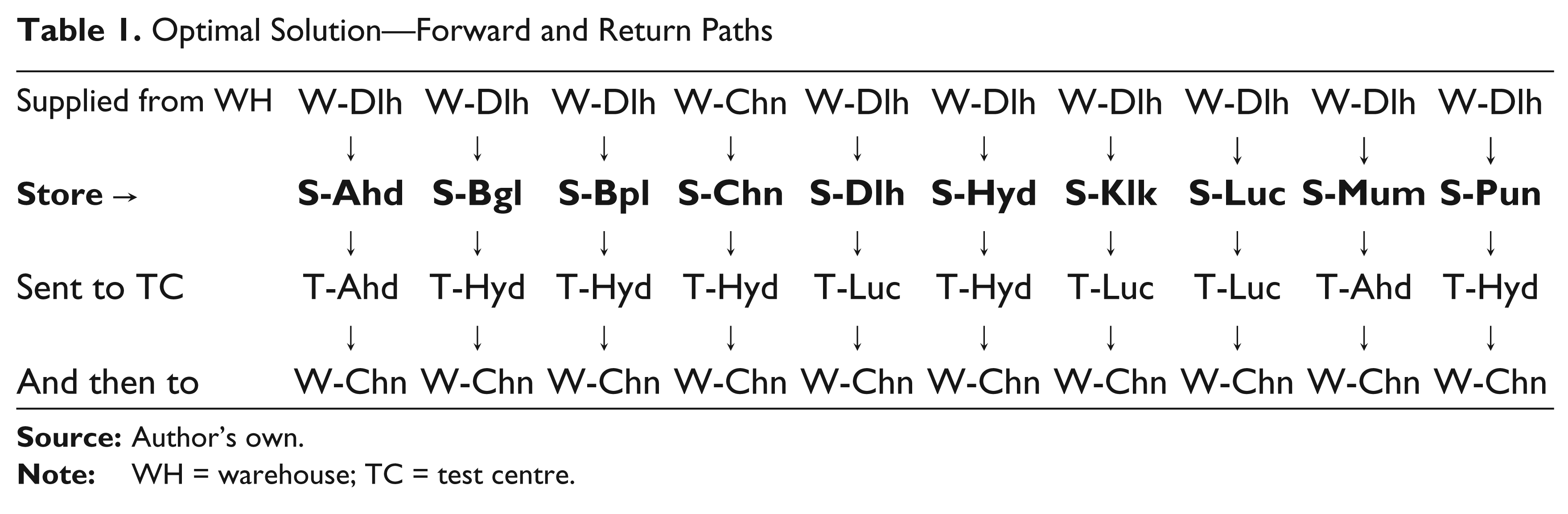
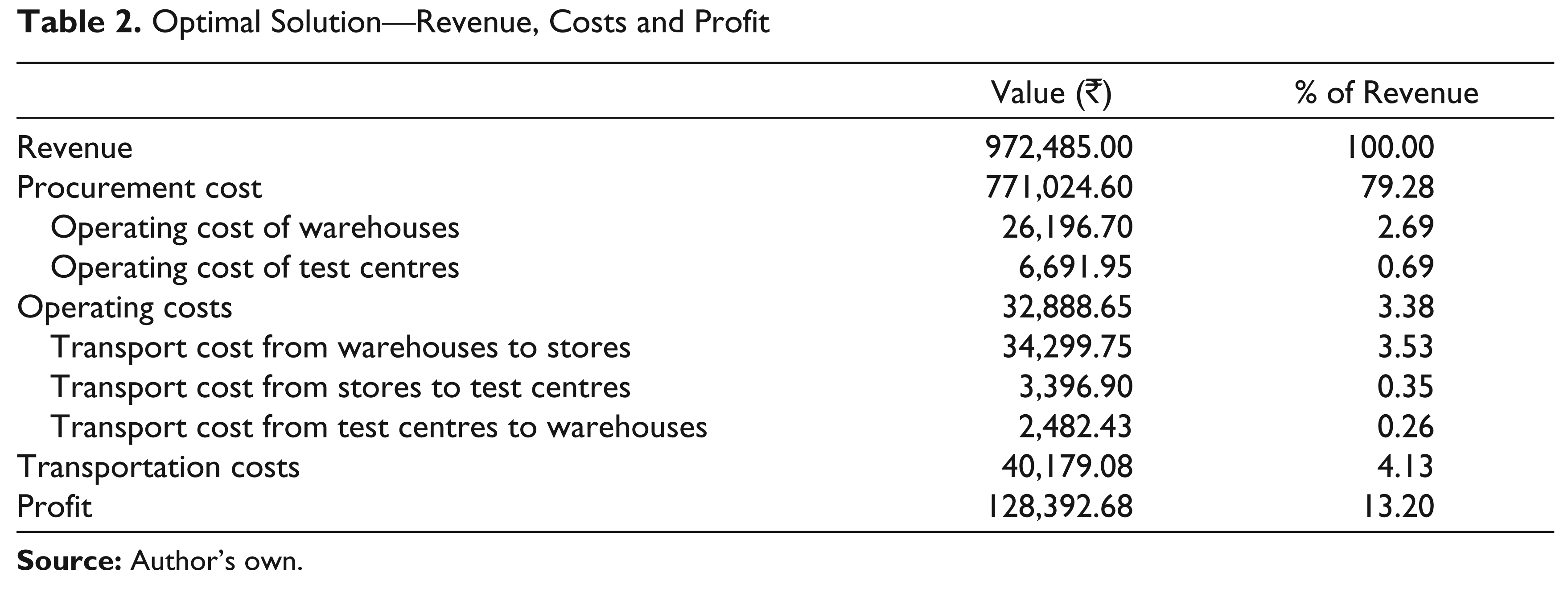
According to the LINGO solution, the company should operate only two warehouses—W-Dlh and W-Chn—and three test centres, T-Ahd, T-Hyd and T-Luc. The table shows the forward path to each store and the return path from each store. For example, store S-Ahd is supplied from W-Dlh and sends the product returns to T-Ahd, which then sends the re-stockable returns to W-Chn. The LINGO solution also reports the revenues, costs and profit per period as shown in Table 2.

Table 2.

Optimal Solution—Revenue, Costs and Profit

	Value (₹)	% of Revenue
Revenue	972,485.00	100.00
Procurement cost	771,024.60	79.28
Operating cost of warehouses	26,196.70	2.69
Operating cost of test centres	6,691.95	0.69
Operating costs	32,888.65	3.38
Transport cost from warehouses to stores	34,299.75	3.53
Transport cost from stores to test centres	3,396.90	0.35
Transport cost from test centres to warehouses	2,482.43	0.26
Transportation costs	40,179.08	4.13
Profit	128,392.68	13.20

Source: Author’s own.

Interestingly, all the product returns are sent back to only one warehouse, namely, W-Chn, although another warehouse, W-Dlh, is also operating. W-Dlh receives only fresh products from the manufacturers and sends these to all stores but to S-Chn.

Discussion and Sensitivity Analysis

We now study the sensitivity of the optimal solution to some of the parameter values assumed in our problem. The initial set of parameter values and the optimal solution presented in the previous section is taken as the baseline for all such analysis in this section.

The observation mentioned at the end of the previous section may be intriguing at first sight but a closer look highlights that it is attempting to take advantage of a lower procurement price at W-Dlh vis-à-vis W-Chn, which overrides the saving in transportation cost that could be obtained by sending the re-stockable returns from each of the test centre to a warehouse with the least transportation cost.

Effect of Changing ‘Fraction’

This raises another important issue for consideration: would it be fair to send all re-stockable returns to one and all fresh products to another warehouse, as suggested by the previous optimal solution? In case the management of the company decides not to send more than a pre-decided maximum ‘Fraction’ of re-stockable returns to any warehouse, this can be achieved by adding the following simple constraint for each warehouse:

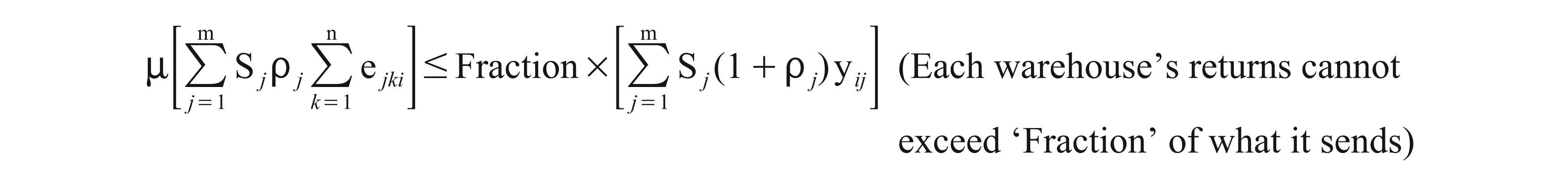
\begin{array}{l} μ [\sum_{j = 1}^{m} S_{j} ρ_{j} \sum_{k = 1}^{n} e_{j k i}] \leq F r a c t i o n \times [\sum_{j = 1}^{m} S_{j} (1 + ρ_{j}) y_{i j}] (E a c h w a r e h o u s e ΄ s r e t u r n s c a n n o t \\ e x c e e d ΄ F r a c t i o n ΄ o f w h a t i t s e n d s) \end{array}

Table 3 shows the revenue per period for the optimal solution under different values of the ‘Fraction’ as well as the various costs—procurement cost, total operating costs (of both warehouses and test centres) and total transportation costs (for both forward and reverse logistics)—and the profit per period as a percentage of the revenue. It also shows the candidate warehouse and test centre locations where these facilities need to be operating using only the binary values of the decision variables w_i and x_k.

Table 3.

Sensitivity to the Maximum ‘Fraction’ of Re-stockable Returns to a Warehouse

‘Fraction’	Warehouses	Test Centres	Revenue Value (₹)	% of Revenue
‘Fraction’	Warehouses	Test Centres	Revenue Value (₹)	Proc. Cost	Optg Cost	Trans Cost	Profit
1	(0,0,1,1,0,0)	(1,0,1,0,1,0)	972,485	79.28	3.38	4.13	13.20
0.5	(0,0,1,1,0,0)	(1,0,1,0,1,0)	972,485	79.40	3.38	4.10	13.12
0.25	(0,0,0,1,0,0)	(1,0,1,0,1,0)	972,485	78.84	3.26	4.90	13.00
0.1	(0,0,0,1,0,0)	(1,0,1,0,1,0)	972,485	78.84	3.26	4.90	13.00

Source: Author’s own.

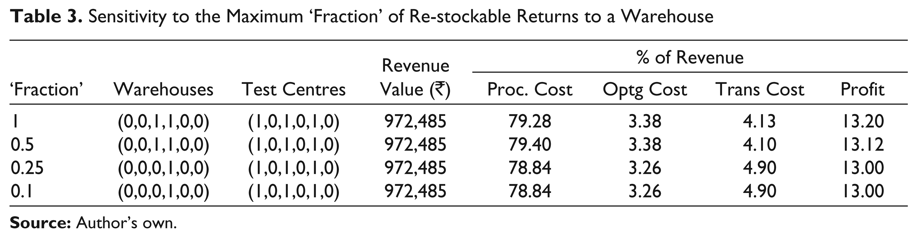
As the ‘Fraction’ allowed is reduced, at first the procurement cost increases slightly as the constraint on returns distributes the returns to more warehouses (among the operating warehouses) and increases the consequent procurement cost. As the ‘Fraction’ is reduced further, the number of operating warehouses reduces with consequent higher flows through the retained warehouses to accommodate the reduced ‘Fraction’ allowed of returns. All through these reductions in ‘Fraction’, the profit margin falls, first as procurement costs increase and then as both procurement and transportation costs increase. There is no effect on the test centres and that on the warehouses is that of closing down an operating warehouse, thus showing the robustness of the optimal solution to changes in ‘Fraction’.

Table 4.

Sensitivity to Changes in Demands

Demand Change	Warehouses	Test Centres	Revenue Value (₹)	% of Revenue
Demand Change	Warehouses	Test Centres	Revenue Value (₹)	Proc. Cost	Optg Cost	Trans Cost	Profit
0	(0,0,1,1,0,0)	(1,0,1,0,1,0)	972,485	79.28	3.38	4.13	13.20
100.00%	(0,0,1,1,0,0)	(1,0,1,0,1,0)	1,944,970	79.28	3.04	4.13	13.54
200.00%	(0,0,1,1,0,0)	(1,1,1,0,1,0)	2,917,455	79.28	2.95	4.10	13.66
400.00%	(0,0,1,1,0,0)	(1,1,1,0,1,0)	4,862,425	79.28	2.85	4.10	13.76
500.00%	(0,0,1,1,0,0)	(1,1,1,1,1,0)	5,834,910	79.28	2.89	4.04	13.79
600.00%	(0,0,1,1,0,0)	(1,1,1,1,1,1)	6,807,395	79.28	2.92	3.99	13.81
–10.00%	(0,0,1,1,0,0)	(1,0,1,0,1,0)	875,237	79.28	3.46	4.13	13.13
–25.00%	(0,0,1,1,0,0)	(0,0,1,0,1,0)	729,364	79.28	3.56	4.17	12.98
–50.00%	(0,0,1,1,0,0)	(0,0,1,0,1,0)	486,243	79.28	3.99	4.17	12.55
–75.00%	(0,0,0,1,0,0)	(0,0,0,0,1,0)	243,121	78.84	4.48	5.06	11.62
–90.00%	(0,0,0,1,0,0)	(0,0,0,0,1,0)	97,249	78.84	7.13	5.06	8.97
–99.00%	(0,0,0,0,1,0)	(0,0,0,0,1,0)	9,725	88.40	15.44	6.00	–9.83

Source: Author’s own.

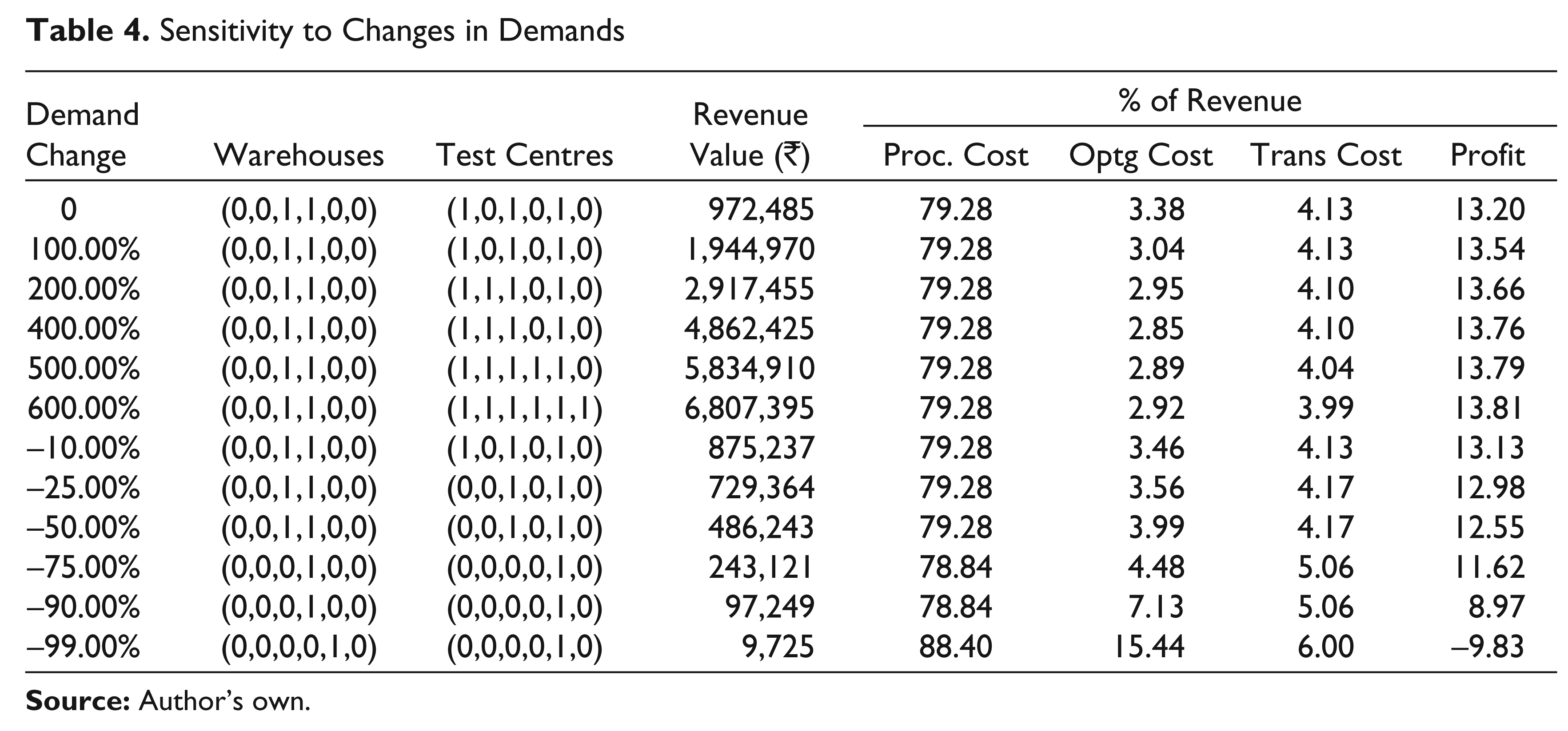
Effect of Changes in Demand

Table 4 studies the sensitivity of the optimal solution to changes in demand from the retail stores. If the demand changes by as much as +100 per cent or –50 per cent, there is no change in the warehouse or test centre locations. As the demand increases by more than +200 per cent, more test centres become viable and as demand falls by more than 50 per cent, only some of the operating test centres and warehouses are retained. In the extreme case when demand falls by more than –99 per cent, does a new warehouse location become better suited than of the existing ones—again highlighting the relative robustness of the optimal solution to moderate changes in demands.

Table 5.

Sensitivity to Changes in Selling Price

Selling Price Change	Warehouses	Test Centres	Revenue Value (₹)	% of Revenue
Selling Price Change	Warehouses	Test Centres	Revenue Value (₹)	Proc. Cost	Optg Cost	Trans Cost	Profit
0	(0,0,1,1,0,0)	(1,0,1,0,1,0)	972,485	79.28	3.38	4.13	13.20
50.00%	(0,0,1,1,0,0)	(1,0,1,0,1,0)	1,449,485	53.19	2.27	2.77	41.77
100.00%	(0,0,1,1,0,0)	(1,0,1,0,1,0)	1,926,485	40.02	1.71	2.09	56.18
–10.00%	(0,0,1,1,0,0)	(1,0,1,0,1,0)	877,085	87.91	3.75	4.58	3.76
–25.00%	(0,0,1,1,0,0)	(1,0,1,0,1,0)	733,985	105.05	4.48	5.47	–15.00
–50.00%	(0,0,1,1,0,0)	(1,0,1,0,1,0)	495,485	155.61	6.64	8.11	–70.36

Source: Author’s own.

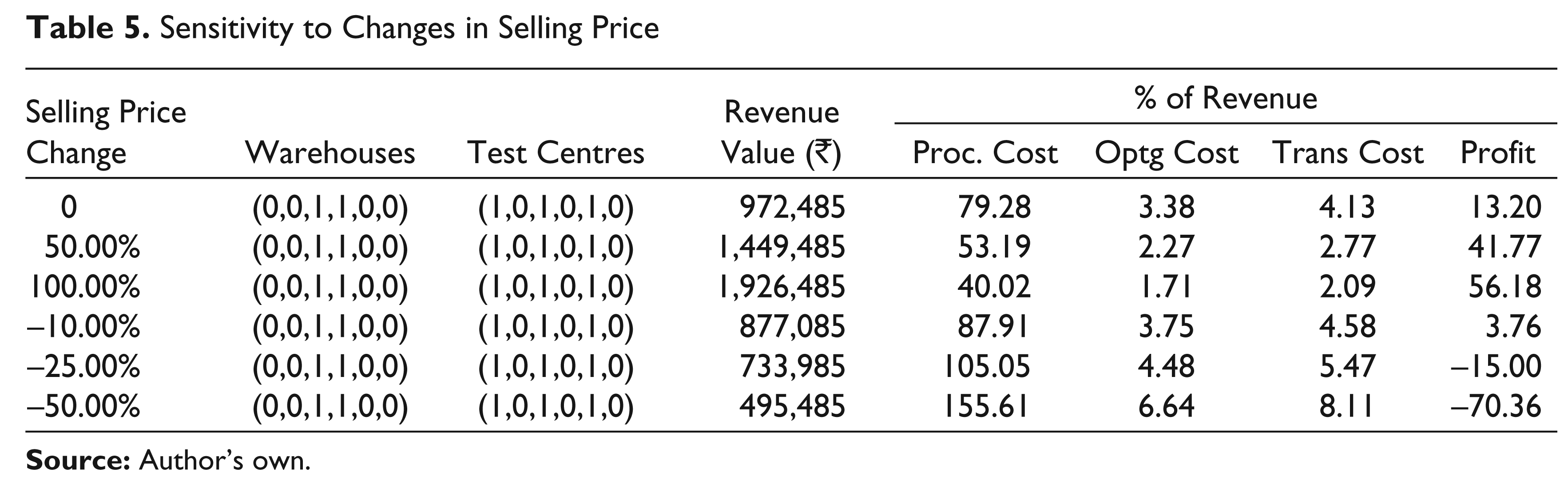
Effect of Changes in Selling Price

In our model, we have made a reasonable assumption that the selling prices across all retail stores are equal even though the procurement prices at different warehouses (including freight inwards) are different. Table 5 shows the optimal solution for different changes in the selling price. If the selling price alone changes by as much as +100 per cent or –50 per cent, there is no change in the optimal location of warehouses and test centres. Of course, the profitability of the supply chain is highly sensitive to selling price changes—for example, a 50 per cent increase in the selling price causes a more than 200 per cent increase in profit margin.

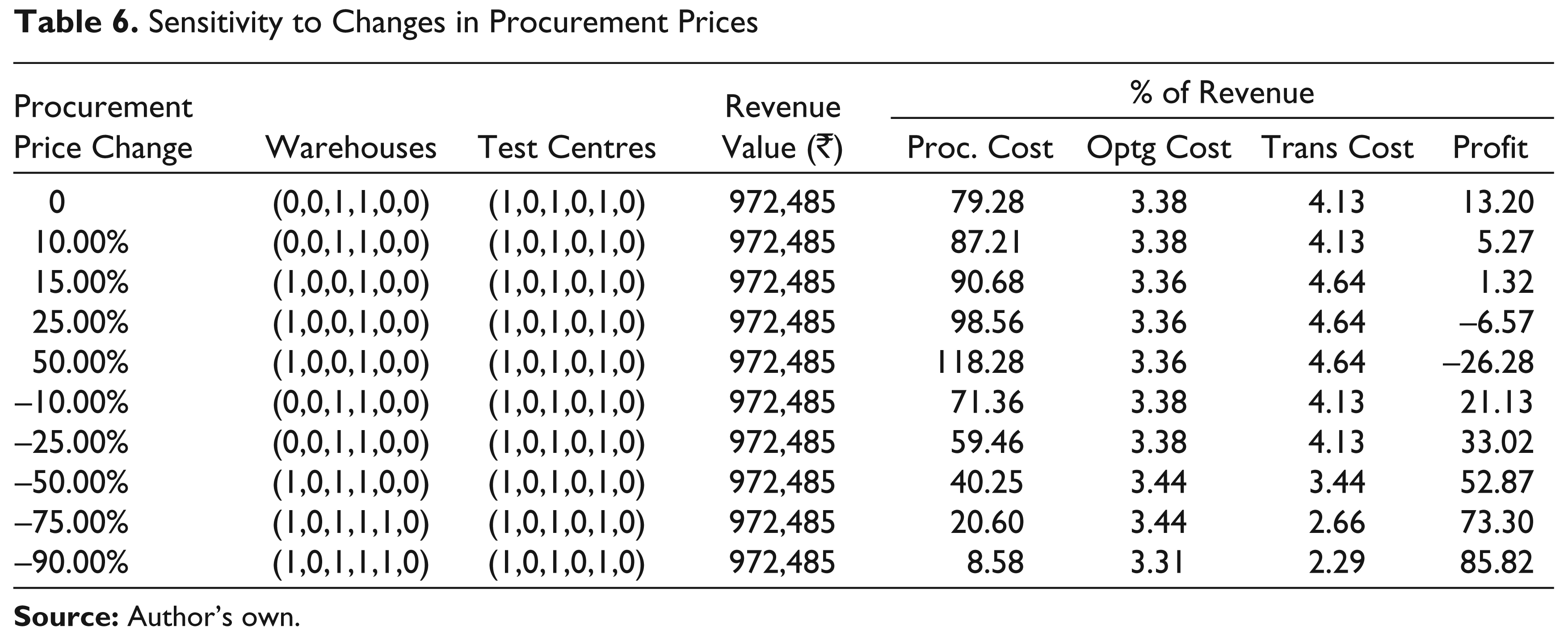
Effect of Changes in Procurement Prices

Table 6, which captures the effect of procurement price changes, shows that additional warehouses would be needed if the procurement prices fell by 50 per cent or more. This may be because, with a constant percentage decline in procurement prices, the procurement prices at different warehouses would tend to equalize and warehouse location would largely be decided by the trade-off between the operating and transportation costs alone.

On the other hand, if the procurement prices increased by, say, 15 per cent, the optimal choice of warehouses would change (although the number of warehouses operating would not change) and the supply chain operations would become less profitable under such circumstances. This could again be because the difference in procurement prices at different warehouse locations becomes larger and warehouse location tends to be made on lower procurement prices than on the trade-off between the operating and transportation costs alone.

However, for small changes in procurement prices up to 10 per cent, the optimal network design would remain unchanged. In either case—that, is for procurement price increases or decreases—the test centre choices are not affected at all.

Table 6.

Sensitivity to Changes in Procurement Prices

Procurement Price Change	Warehouses	Test Centres	Revenue Value (₹)	% of Revenue
Procurement Price Change	Warehouses	Test Centres	Revenue Value (₹)	Proc. Cost	Optg Cost	Trans Cost	Profit
0	(0,0,1,1,0,0)	(1,0,1,0,1,0)	972,485	79.28	3.38	4.13	13.20
10.00%	(0,0,1,1,0,0)	(1,0,1,0,1,0)	972,485	87.21	3.38	4.13	5.27
15.00%	(1,0,0,1,0,0)	(1,0,1,0,1,0)	972,485	90.68	3.36	4.64	1.32
25.00%	(1,0,0,1,0,0)	(1,0,1,0,1,0)	972,485	98.56	3.36	4.64	–6.57
50.00%	(1,0,0,1,0,0)	(1,0,1,0,1,0)	972,485	118.28	3.36	4.64	–26.28
–10.00%	(0,0,1,1,0,0)	(1,0,1,0,1,0)	972,485	71.36	3.38	4.13	21.13
–25.00%	(0,0,1,1,0,0)	(1,0,1,0,1,0)	972,485	59.46	3.38	4.13	33.02
–50.00%	(1,0,1,1,0,0)	(1,0,1,0,1,0)	972,485	40.25	3.44	3.44	52.87
–75.00%	(1,0,1,1,1,0)	(1,0,1,0,1,0)	972,485	20.60	3.44	2.66	73.30
–90.00%	(1,0,1,1,1,0)	(1,0,1,0,1,0)	972,485	8.58	3.31	2.29	85.82

Source: Author’s own.

Table 7.

Sensitivity to Changes in Discounted Prices

Discounted Price Change	Warehouses	Test Centres	Revenue Value (₹)	% of Revenue
Discounted Price Change	Warehouses	Test Centres	Revenue Value (₹)	Proc. Cost	Optg Cost	Trans Cost	Profit
0	(0,0,1,1,0,0)	(1,0,1,0,1,0)	972,485	79.28	3.38	4.13	13.20
100.00%	(0,0,1,1,0,0)	(1,0,1,0,1,0)	990,970	77.81	3.32	4.05	14.82
–50.00%	(0,0,1,1,0,0)	(1,0,1,0,1,0)	963,243	80.04	3.41	4.17	12.37
–100.00%	(0,0,1,1,0,0)	(1,0,1,0,1,0)	954,000	80.82	3.45	4.21	11.52

Source: Author’s own.

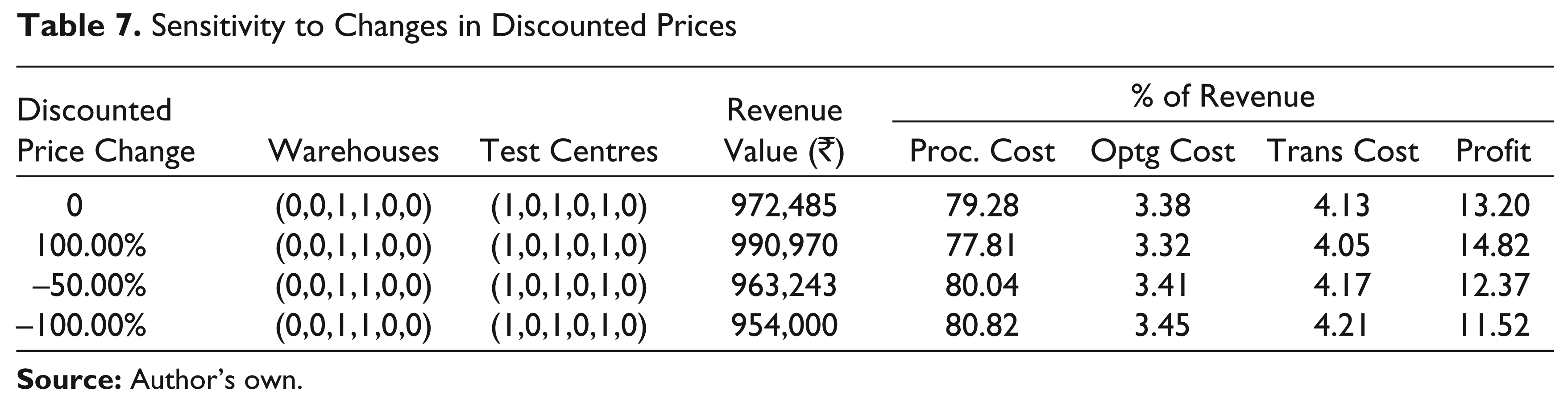
Effect of Changes in Discounted Prices

As the quantities of the returned products sold in the secondary market are relatively small, the network design is not affected at all by changes in discounted prices. This can be seen from Table 7, which shows the optimal solution for different percentages of this change.

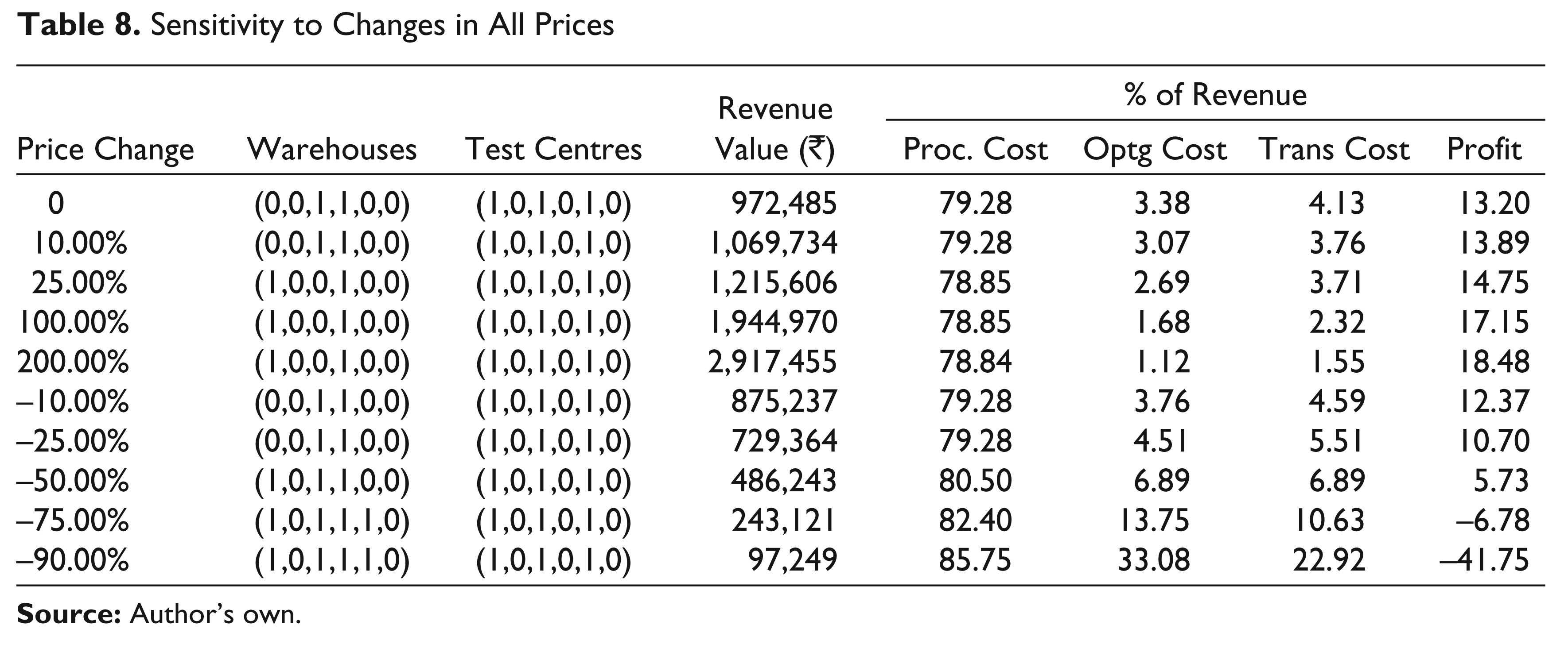
Effect of Changes in All Prices Simultaneously

In case all the three prices changed by an equal percentage, the network design is primarily affected by procurement price changes. This can be seen from Table 8, where the sensitivity of the optimal solution to simultaneous changes in all three prices is presented. A comparison with Table 6 confirms that the changes in network design are driven by the changes in procurement prices alone.

Effect of Changing Return Rate (ρ)

An increase in the return rate increases the secondary sales (for the same primary sales), and so increases the revenue but reduces the profit margin. Table 9 also shows that the locations of warehouses and test centres are not affected if the return rate increased by as much as 100 per cent; however, an increase of 200 per cent would require the operation of an additional warehouse and an additional test centre and yet the supply chain would become unprofitable.

Table 8.

Sensitivity to Changes in All Prices

Price Change	Warehouses	Test Centres	Revenue Value (₹)	% of Revenue
Price Change	Warehouses	Test Centres	Revenue Value (₹)	Proc. Cost	Optg Cost	Trans Cost	Profit
0	(0,0,1,1,0,0)	(1,0,1,0,1,0)	972,485	79.28	3.38	4.13	13.20
10.00%	(0,0,1,1,0,0)	(1,0,1,0,1,0)	1,069,734	79.28	3.07	3.76	13.89
25.00%	(1,0,0,1,0,0)	(1,0,1,0,1,0)	1,215,606	78.85	2.69	3.71	14.75
100.00%	(1,0,0,1,0,0)	(1,0,1,0,1,0)	1,944,970	78.85	1.68	2.32	17.15
200.00%	(1,0,0,1,0,0)	(1,0,1,0,1,0)	2,917,455	78.84	1.12	1.55	18.48
–10.00%	(0,0,1,1,0,0)	(1,0,1,0,1,0)	875,237	79.28	3.76	4.59	12.37
–25.00%	(0,0,1,1,0,0)	(1,0,1,0,1,0)	729,364	79.28	4.51	5.51	10.70
–50.00%	(1,0,1,1,0,0)	(1,0,1,0,1,0)	486,243	80.50	6.89	6.89	5.73
–75.00%	(1,0,1,1,1,0)	(1,0,1,0,1,0)	243,121	82.40	13.75	10.63	–6.78
–90.00%	(1,0,1,1,1,0)	(1,0,1,0,1,0)	97,249	85.75	33.08	22.92	–41.75

Source: Author’s own.

Table 9.

Sensitivity to Changes in Return Rates (ρ)

Return Rate Change	Warehouses	Test Centres	Revenue Value (₹)	% of Revenue
Return Rate Change	Warehouses	Test Centres	Revenue Value (₹)	Proc. Cost	Optg Cost	Trans Cost	Profit
0	(0,0,1,1,0,0)	(1,0,1,0,1,0)	972,485	79.28	3.38	4.13	13.20
50.00%	(0,0,1,1,0,0)	(1,0,1,0,1,0)	981,728	81.76	3.79	4.64	9.81
100.00%	(0,0,1,1,0,0)	(1,0,1,0,1,0)	990,970	84.20	4.19	5.14	6.48
200.00%	(1,0,1,1,0,0)	(1,1,1,0,1,0)	1,009,455	89.41	5.13	5.57	–0.10
–10.00%	(0,0,1,1,0,0)	(1,0,1,0,1,0)	970,637	78.78	3.30	4.03	13.89
–25.00%	(1,0,0,1,0,0)	(1,0,1,0,1,0)	967,864	77.48	3.17	4.39	14.96
–40.00%	(1,0,0,1,0,0)	(1,0,1,0,0,0)	965,091	76.73	3.01	4.24	16.01
–50.00%	(0,0,0,1,0,0)	(0,0,0,0,1,0)	963,243	76.11	2.75	4.41	16.73

Source: Author’s own.

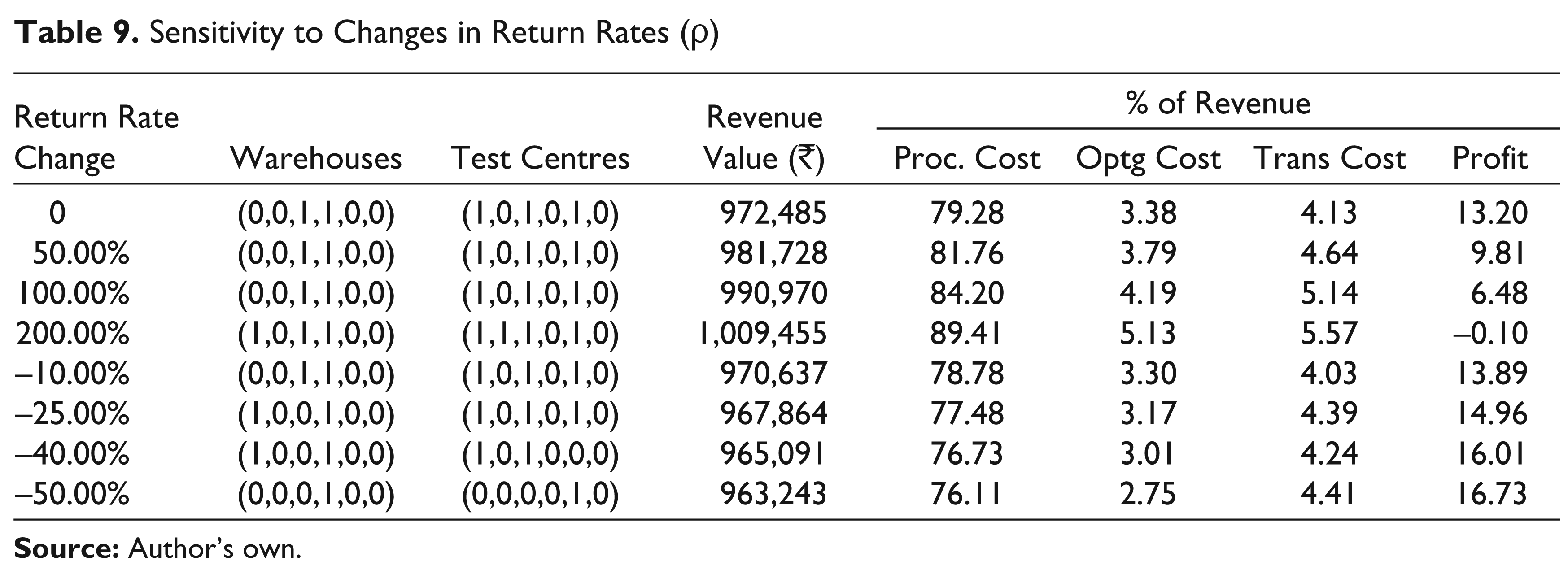
Interestingly, a drop of 25 per cent in the return rate would require the relocation of one warehouse and further drops would require the closing down of, first, test centres and then, warehouses as well. For very small return rates, only one warehouse and one test centre from the baseline network need to operate.

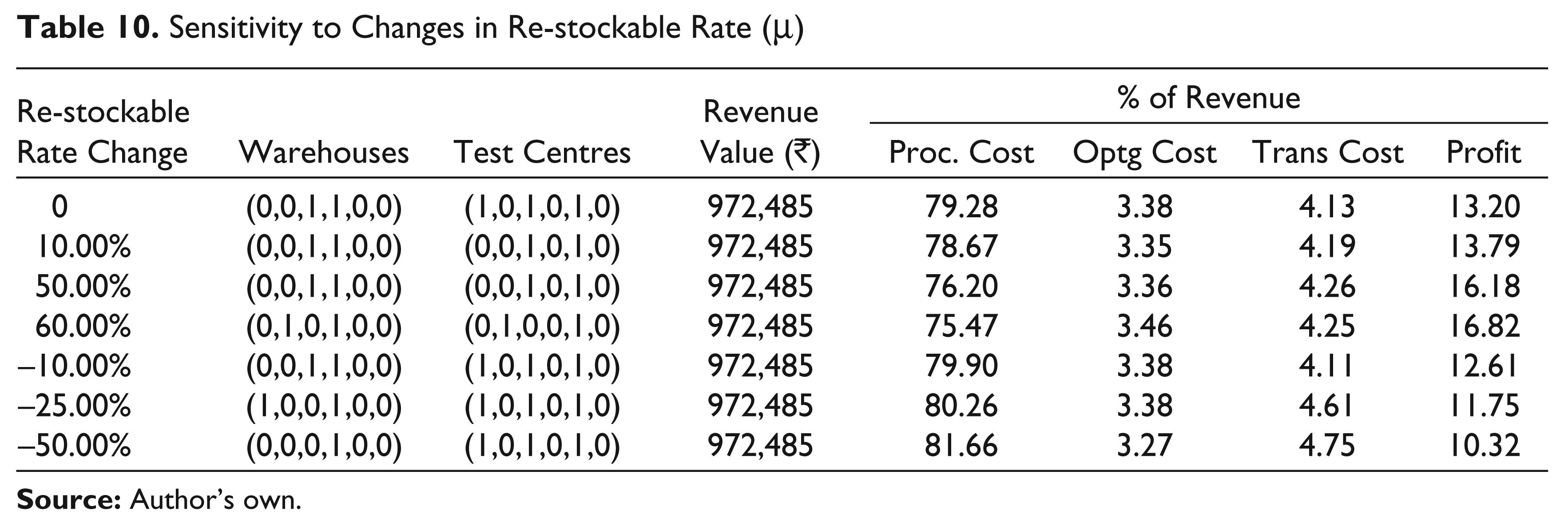
Effect of Changing Re-stockable Rate (μ)

Table 10 reveals that even a small 10 per cent increase in re-stockable rate enables the closure of one test centre, while a moderate increase of 60 per cent causes a relocation of both warehouses and test centres. Similarly, a decrease of 25 per cent in this rate requires a relocation of one warehouse and a decrease of 50 per cent enables the closure of one warehouse. In the baseline model, the re-stockable rate emerges as a key parameter affecting the design of the supply chain network.

Table 10.

Sensitivity to Changes in Re-stockable Rate (μ)

Re-stockable Rate Change	Warehouses	Test Centres	Revenue Value (₹)	% of Revenue
Re-stockable Rate Change	Warehouses	Test Centres	Revenue Value (₹)	Proc. Cost	Optg Cost	Trans Cost	Profit
0	(0,0,1,1,0,0)	(1,0,1,0,1,0)	972,485	79.28	3.38	4.13	13.20
10.00%	(0,0,1,1,0,0)	(0,0,1,0,1,0)	972,485	78.67	3.35	4.19	13.79
50.00%	(0,0,1,1,0,0)	(0,0,1,0,1,0)	972,485	76.20	3.36	4.26	16.18
60.00%	(0,1,0,1,0,0)	(0,1,0,0,1,0)	972,485	75.47	3.46	4.25	16.82
–10.00%	(0,0,1,1,0,0)	(1,0,1,0,1,0)	972,485	79.90	3.38	4.11	12.61
–25.00%	(1,0,0,1,0,0)	(1,0,1,0,1,0)	972,485	80.26	3.38	4.61	11.75
–50.00%	(0,0,0,1,0,0)	(1,0,1,0,1,0)	972,485	81.66	3.27	4.75	10.32

Source: Author’s own.

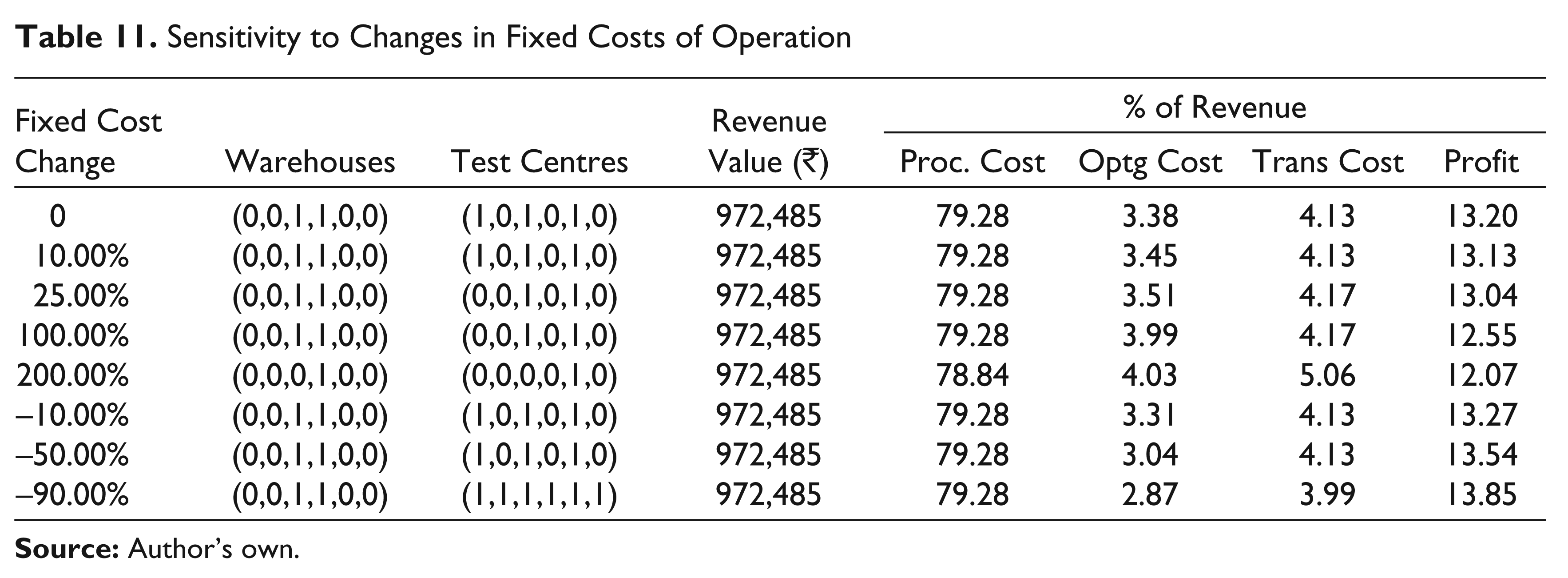
Effect of Changing Fixed Costs (for both warehouses and test centres)

The effect of a change in fixed costs of operating warehouses and test centres is reflected in Table 11, according to which a moderate increase of 25 per cent or 100 per cent would require the closing down of one test centre, while a large increase of 200 per cent would require the closure of all but one warehouse and all but one test centre. The consequent increase in transportation cost is moderated by a reduction in production cost as only the warehouse with the least procurement price is retained. The table also shows that moderate decreases in fixed costs have no effect on the network design, but very large decreases would mandate operation of all test centres to take advantage of lower fixed costs as well as transportation costs. The operation of warehouses, however, is not affected as they continue to exploit the procurement price differentials.

Table 11.

Sensitivity to Changes in Fixed Costs of Operation

Fixed Cost Change	Warehouses	Test Centres	Revenue Value (₹)	% of Revenue
Fixed Cost Change	Warehouses	Test Centres	Revenue Value (₹)	Proc. Cost	Optg Cost	Trans Cost	Profit
0	(0,0,1,1,0,0)	(1,0,1,0,1,0)	972,485	79.28	3.38	4.13	13.20
10.00%	(0,0,1,1,0,0)	(1,0,1,0,1,0)	972,485	79.28	3.45	4.13	13.13
25.00%	(0,0,1,1,0,0)	(0,0,1,0,1,0)	972,485	79.28	3.51	4.17	13.04
100.00%	(0,0,1,1,0,0)	(0,0,1,0,1,0)	972,485	79.28	3.99	4.17	12.55
200.00%	(0,0,0,1,0,0)	(0,0,0,0,1,0)	972,485	78.84	4.03	5.06	12.07
–10.00%	(0,0,1,1,0,0)	(1,0,1,0,1,0)	972,485	79.28	3.31	4.13	13.27
–50.00%	(0,0,1,1,0,0)	(1,0,1,0,1,0)	972,485	79.28	3.04	4.13	13.54
–90.00%	(0,0,1,1,0,0)	(1,1,1,1,1,1)	972,485	79.28	2.87	3.99	13.85

Source: Author’s own.

Table 12.

Sensitivity to Changes in Variable Costs of Operation

Variable Cost Change	Warehouses	Test Centres	Revenue Value (₹)	% of Revenue
Variable Cost Change	Warehouses	Test Centres	Revenue Value (₹)	Proc. Cost	Optg Cost	Trans Cost	Profit
0	(0,0,1,1,0,0)	(1,0,1,0,1,0)	972,485	79.28	3.38	4.13	13.20
100.00%	(0,0,1,1,0,0)	(1,0,1,0,1,0)	972,485	79.28	6.08	4.14	10.50
200.00%	(0,0,1,1,0,0)	(0,0,1,0,1,0)	972,485	79.28	8.72	4.20	7.80
400.00%	(0,0,1,1,0,0)	(0,0,1,0,1,0)	972,485	79.28	14.04	4.25	2.43
450.00%	(0,0,0,1,1,0)	(1,0,0,0,1,0)	972,485	78.85	15.25	4.81	1.09
600.00%	(0,0,0,1,1,0)	(1,0,0,0,1,0)	972,485	78.85	19.26	4.81	–2.91
700.00%	(0,0,1,1,1,0)	(1,0,0,0,1,0)	972,485	79.79	21.70	4.08	–5.56
900.00%	(0,0,1,1,1,0)	(1,0,0,0,1,0)	972,485	79.79	26.93	4.08	–10.80
–90.00%	(0,0,1,1,0,0)	(1,0,1,0,1,0)	972,485	79.28	0.95	4.13	15.64

Source: Author’s own.

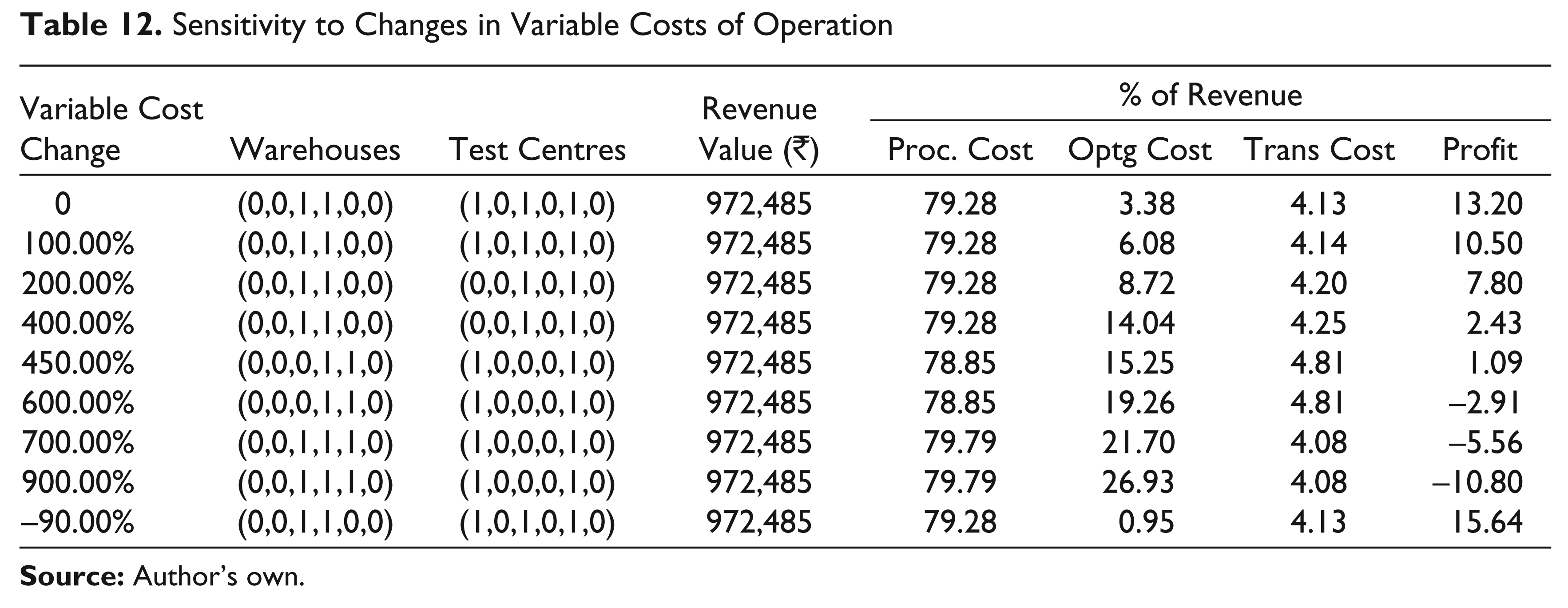
Effect of Changing Variable Costs (for both warehouses and test centres)

In case the variable costs of operating warehouses and test centres change rather than the fixed costs, the network designs should be according to the Table 12. Moderate increases up to 100 per cent have no effect, while a 200 per cent or 400 per cent increase would require the closure of one test centre. Surprisingly, an increase of, say, 450 per cent or 600 per cent requires the relocation of one warehouse and one test centre as such large increases change the warehouse location preference, which is based on the sum of procurement price and the variable cost at the respective warehouse. Still higher increases in variable costs tend to stabilize the network design. As variable cost differentials are not very large to begin with, reductions in variable costs have no effect on the network design.

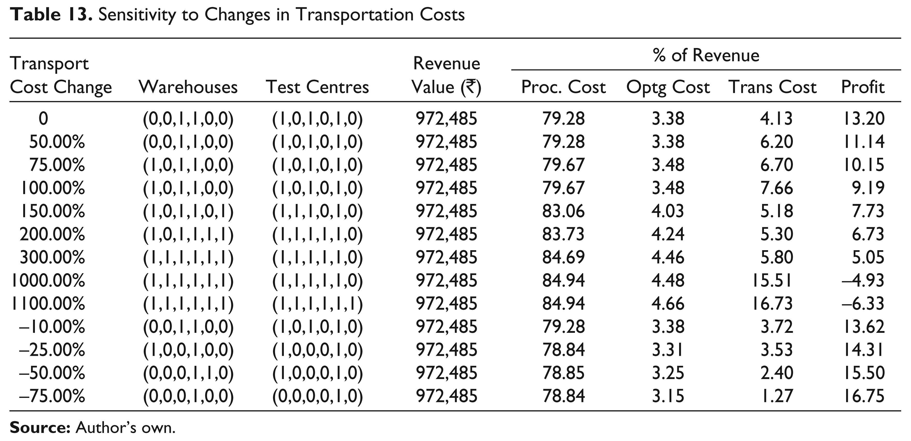
Effect of Changing Transportation Costs

Table 13 shows that as transportation costs increase, additional warehouses are first introduced—for example, a third warehouse is introduced when the transportation costs increase by 75 per cent—followed by further additions of both test centres and warehouses. For very high increases in transportation costs, as expected, all warehouses and test centres need to operate.

A small decrease—say of 10 per cent—in transportation costs has no effect on the optimal design of the supply chain network, but a moderate decrease of 25 per cent causes a relocation of a warehouse and closure of a test centre. As transportation costs reduce, warehouse locations are influenced more by lower procurement prices. Further decreases may require relocations of warehouses and eventually, when transportation costs have declined by 75 per cent, only one warehouse and one test centre would be needed. Substantial decreases in transportation costs and similar increases in fixed costs of operation are nothing but two sides of the same coin and have similar effects.

Conclusion

As pointed out in the review of literature, some authors have modelled integrated reverse logistics network design problem as an MILP or as an MIP—whereas we have used binary ILP. The formulation is simpler and ILP software is relatively easy to obtain, particularly for not very large problems. In spite of this simplification, the formulation retains the flexibility to handle different types of products and their supply chains through adjustments of the parameter values. Such adjustments could easily handle products with different characteristics—commodity products, niche products, high and low-value products, etc.

Table 13.

Sensitivity to Changes in Transportation Costs

Transport Cost Change	Warehouses	Test Centres	Revenue Value (₹)	% of Revenue
Transport Cost Change	Warehouses	Test Centres	Revenue Value (₹)	Proc. Cost	Optg Cost	Trans Cost	Profit
0	(0,0,1,1,0,0)	(1,0,1,0,1,0)	972,485	79.28	3.38	4.13	13.20
50.00%	(0,0,1,1,0,0)	(1,0,1,0,1,0)	972,485	79.28	3.38	6.20	11.14
75.00%	(1,0,1,1,0,0)	(1,0,1,0,1,0)	972,485	79.67	3.48	6.70	10.15
100.00%	(1,0,1,1,0,0)	(1,0,1,0,1,0)	972,485	79.67	3.48	7.66	9.19
150.00%	(1,0,1,1,0,1)	(1,1,1,0,1,0)	972,485	83.06	4.03	5.18	7.73
200.00%	(1,0,1,1,1,1)	(1,1,1,1,1,0)	972,485	83.73	4.24	5.30	6.73
300.00%	(1,1,1,1,1,1)	(1,1,1,1,1,0)	972,485	84.69	4.46	5.80	5.05
1000.00%	(1,1,1,1,1,1)	(1,1,1,1,1,0)	972,485	84.94	4.48	15.51	–4.93
1100.00%	(1,1,1,1,1,1)	(1,1,1,1,1,1)	972,485	84.94	4.66	16.73	–6.33
–10.00%	(0,0,1,1,0,0)	(1,0,1,0,1,0)	972,485	79.28	3.38	3.72	13.62
–25.00%	(1,0,0,1,0,0)	(1,0,0,0,1,0)	972,485	78.84	3.31	3.53	14.31
–50.00%	(0,0,0,1,1,0)	(1,0,0,0,1,0)	972,485	78.85	3.25	2.40	15.50
–75.00%	(0,0,0,1,0,0)	(0,0,0,0,1,0)	972,485	78.84	3.15	1.27	16.75

Source: Author’s own.

Extensive sensitivity analysis of our model reveals the relative robustness of the optimal design to small and even moderate changes in most parameter values. Surprisingly, we found greater sensitivity to procurement price changes vis-à-vis changes in selling prices or discounted prices, and also relatively high sensitivity to the re-stockable rate. The model also revealed its ability to change procurement decisions even within the framework of existing warehouses and test centres.

In a complex decision problem with a large number of parameters, it is not always straightforward to find the effect of a change in some parameter value. Modelling has a normative as well as a descriptive role in such situations. For example, our baseline decision problem involved the establishment of two warehouses, but all product returns were routed to only one of the two warehouses, whereas all retail stores, except a local one, were required to get their supplies from the other warehouse. The role of procurement price differences was thus clearly brought to light by the model.

The model formulated here could be easily adapted to situations where the selling price at each retail store is different or the procurement price at each warehouse (including freight inward) is a constant or variations thereof. In some cases, there could be some costs involved in donation to charities or throwaways, and minor changes in the model could easily accommodate such changes. We have considered the supply chain from warehouse onwards. It could be expanded to include other echelons in the supply chain like manufacturers and even their suppliers. However, we have taken the average sales per period in a retail store as known and as a constant. In reality, it is stochastic and so could be the prices used in the model. For some products with large uncertainty in demand and prices, this could be a limitation in the use of deterministic models.

In this article, we have modelled an efficient supply chain, where the effect of time on the performance of the supply chain has been ignored. It is possible to include opportunity costs in the objective function to reflect the effect of time on ordering and delivery; such a model could then handle both efficient and responsive supply chains. Often, the size of such decision problems is very large and it may be difficult to obtain the optimal solution. Development of good heuristics to solve large problems should prove immensely useful to practitioners.

Footnotes

Appendix

Parameters:

μ = 0.45; ν = 0.25

References

Abe

, & Ye

(2013). Building resilient supply chains against natural disasters: The cases of Japan and Thailand. Global Business Review, 14(4), 567–586.

Akcali

, Cetinkaya

, & Uster

(2009). Network design for reverse and closed-loop supply chains: An annotated bibliography of models and solution approaches. Networks, 53(3), 231–248.

Amiri

(2006). Designing a distribution network in a supply chain system: Formulation and efficient solution procedure. European Journal of Operational Research, 171(2), 567–576.

Barros

A. I.

, Dekker

, & Scholten

(1998). A two-level network for recycling sand: A case study. European Journal of Operational Research, 110(2), 199–214.

Carter

C. R.

, & Ellram

L. M.

(1998). Reverse logistics: A review of the literature and framework for future investigation. Journal of Business Logistics, 19(1), 85–102.

Das

Kanchan

. (2012). Integrating reverse logistics into the strategic planning of a supply chain. International Journal of Production Research, 50(5), 1438–1456.

Fleischmann

(2000). Quantitative models for reverse logistics (PhD thesis, Erasmus Research Institute of Management, Erasmus University Rotterdam). Available at: http://repub.eur.nl/pub/1044/EPS-2000-002-LIS+FLEISCHMANN.pdf. (Accessed 3 September 2014 ).

Fleischmann

, Bloemhof-Ruwaard

J. M.

, Dekker

, van der Laan

, Van Nunen

J. A. E. E.

, & Van Wassenhove

L. N.

(1997). Quantitative models for reverse logistics: A review. European Journal of Operational Research, 103(1), 1–17.

Guide, Jr

V. D. R.

, Souza

G. C.

, Van Wassenhove

L. N.

, & Blackburn

J. D.

(2006). Time value of commercial product returns. Management Science, 52(8), 1200–1214.

10.

Hsu

H. S.

, Alexander

C. A.

, & Zhu

(2009). Understanding the reverse logistics operations of a retailer: A pilot study. Industrial Management & Data Systems, 109(4), 515–531.

11.

Jayaraman

, Guide Jr

V. D. R.

, & Srivastava

(1999). A closed loop logistics model for remanufacturing. Journal of the Operational Research Society, 50(5), 497–508.

12.

Jayaraman

, Patterson

, & Rolland

(2003). The design of reverse distribution networks: Models and solution procedures. European Journal of Operational Research, 150(2), 128–149.

13.

Khajavi

L. T.

, Seyed-Hosseini

, & Makui

(2011). An integrated forward/reverse logistics network optimization model for multi-stage capacitated supply chain. iBusiness, 3, 229–235.

14.

Krikke

, Kooi

, & Schurr

(1999). Network design in reverse logistics: A quantitative model. In Stahly

(Ed.), New trends in distribution logistics (pp. 45–62). Berlin, Germany: Springer.

15.

Kroon

, & Vrijens

(1995). Returnable containers: An example of reverse logistics. International Journal of Physical Distribution and Logistics Management, 25(2), 56–68.

16.

Lee

Yong Joo

, Baker

, & Jayaraman

(2012). Redesigning an integrated forward-reverse logistics system for a third party service provider: an empirical study. International Journal of Production Research, 50(19), 5615–5634.

17.

Lieckens

, & Vandaele

(2007). Reverse logistics network design with stochastic lead times. Computers & Operations Research, 34, 395–416.

18.

Louwers

, Kip

B. J.

, Peeters

, Souren

, & Flapper

S. D. P.

(1999). A facility location allocation model for re-using carpet materials. Computers and Industrial Engineering, 36(4), 855–869.

19.

Meepetchdee

& Shah

(2007). Logistical network design with robustness and complexity considerations. International Journal of Physical Distribution and Logistics Management, 37(3), 201–222.

20.

Melo

M. T.

, Nickel

, & Saldanha-da-Gama

(2009). Facility location and supply chain management—A review. European Journal of Operational Research, 196(2), 401–412.

21.

Min

, Ko

, & Ko

(2006). A genetic algorithm approach to developing the multi-echelon reverse logistics network for product returns. Omega, 34(1), 56–69.

22.

Ozceylan

& Paksoy

(2013). A mixed integer programming model for a closed-loop supply-chain network. International Journal of Production Research, 51(3), 718–734.

23.

Rogers

D. S.

, Melamed

, & Lembke

R. S.

(2012). Modeling and analysis of reverse logistics. Journal of Business Logistics, 33(2), 107–117.

24.

Rogers

D. S.

& Tibben-Lembke

R. S.

(1999). Going backwards: R L trends & practices. Pittsburgh, PA: Reverse Logistics Executive Council. Available at: http://www.rlec.org/reverse.pdf. (Accessed 3 September, 2014).

25.

Snyder

L. V.

(2006). Facility location under uncertainty: A review. IIE Transactions, 38(7), 537–554.

26.

Srivastava

S. K.

(2007). Green supply chain management: A state of the art literature review. International Journal of Management Reviews, 9(1), 53–80.

27.

Srivastava

S. K.

(2008). Network design for reverse logistics. Omega, 36(4), 535–548.

28.

Stock

J. R.

(1992). Reverse logistics. Oak Brook, IL: Council of Logistics Management.

29.

Stock

J. R.

& Mulki

J. P.

(2009). Product returns processing: An examination of practices of manufacturers, wholesalers/distributors, and retailers. Journal of Business Logistics, 30(1), 33–62.

30.

Tan

A. W. K.

& Kumar

(2006). A decision-making model for reverse logistics in the computer industry. The International Journal of Logistics Management, 17(3), 331–354.

31.

Wadhwa

& Madaan

(2007). Decision making framework for modeling an integrated reverse logistics system. In Bhattacharya

(Ed.), Towards next generation e-government (pp. 131–141). New Delhi: IGI Global Publishing. Available at: http://www.csi-sigegov.org/2/13_417_2.pdf. (Accessed 3 September, 2014.