Volatility Clustering and Leverage Effect in the Indian Forex Market

Abstract

Understanding the patterns of volatility in financial assets is immensely useful in portfolio management process. They are the critical inputs for portfolio selection, asset allocation, asset pricing, portfolio diversification and risk management. This study examines the phenomenon of volatility clustering and leverage effect in exchange rates of four major currencies, namely, US dollar (USD), euro, Japanese yen and pound sterling vis-à-vis Indian rupee (INR) from the vantage point of view of volatility modelling and to assess the forecasting ability using generalized autoregressive conditional heteroskedasticity (GARCH)-class models. Besides, it evaluates the models in terms of out-of-sample forecast accuracy. The study spans for a period of 13 years from 3 January 2000 to 31 December 2012. GARCH (1, 1), exponential GARCH (EGARCH) (1, 1), threshold autoregressive conditional heteroskedasticity (TARCH) (1, 1) and power ARCH (1, 1) models are used in this context. The results show the existence of volatility clustering. No significant leverage effects were evident. Volatility seems to be persistent in nature.

Keywords

Forex market leverage effect stochastic models volatility clustering

Introduction

In the past two decades, volatility measurement is one of the fertile domains of research in financial economics for academic researchers, practitioners, market players, investors and policy makers. Modelling volatility of financial assets is a critical input for portfolio selection, asset allocation, asset pricing, portfolio diversification and risk management. It is an integral part of global risk analysis. A number of models are available to forecast volatility of asset prices. It is a well-known fact that the asset prices are exemplified by typical stylized facts, such as, fat-tails distribution, volatility clustering, seasonality effect, leverage effect, asymmetric effect and so on.

Volatility exhibits persistence, that is, periods of high volatility are followed by periods of high volatility and periods of low volatility are followed by periods of low volatility. This implies that volatility could be used as a predictor of volatility in the subsequent periods. This phenomenon is called ‘volatility clustering’. Volatility tends to react differently on arrival of ‘good’ and ‘bad news’, that is, positive and negative innovations. Black (1976) notes the tendency for negative innovations to generate greater volatility in future periods compared with positive innovations of the same magnitude, a phenomenon that he refers to as the ‘leverage effect’.

Indian rupee (INR) vis-à-vis other currencies particularly the US dollar (USD) has observed constant decline in the recent times. This has made the imports costlier for the Indian economy besides triggering overall domestic inflation and higher current account deficit. Some of the factors (Siddharth & Vinod, 2012) that have caused so include global uncertainty, current account deficit, capital account flows, higher inflation, higher real interest rates and lack of reforms.

There exists a rich literature on volatility modelling supporting the use of generalized autoregressive conditional heteroskedasticity (GARCH)-class models to forecast volatility of asset prices; for example, Akgiray (1989), Pagan and Schwert (1990), Lee (1991), Corhay and Rad (1994), Brailsford and Faff (1996), Andersen and Bollerslev (1998), Brooks (1998), McMillan, Speight and Ap Gwilym (2000), Duan and Zhang (2001), Karmakar (2005), Chan and Fung (2007) and Rashid and Ahmad (2008). However, only few studies exist on modelling volatility of exchange rates. The central aim of this article is to study the phenomenon of volatility clustering and leverage effect in exchange rates of four major currencies, namely, USD, euro, Japanese yen and pound sterling vis-à-vis INR from the vantage point of view of volatility modelling and to assess the forecasting ability using GARCH-class models. Besides, it evaluates the models in terms of out-of-sample forecast accuracy.

The remainder of this article is structured as follows: the next section reviews the existing literature in relation to this study. The third section describes the data and discusses the methodology. The fourth section reports the empirical results and the final section concludes the article.

Literature Review

De Grauwe and Markiewicz (2013) compared two competing approaches, namely, statistical learning and fitness learning, to model foreign exchange market participants’ behaviour. They examined which of the learning approaches is best in terms of replicating the exchange rate dynamics. The study found that both learning methods revealed the fundamental value of the exchange rate in the equilibrium but only fitness learning creates the disconnection phenomenon and only statistical learning replicates volatility clustering. Kamal, Haq, Ghani and Khan (2012) examined the performance of GARCH family models in forecasting the volatility behaviour of the Pakistani FOREX market. The first-order autoregressive behaviour of the FOREX rate was evidenced in GARCH-in-mean (GARCH-M) and exponential GARCH (EGARCH) models while the GARCH-M model supported that previous day FOREX rate affected the current day exchange rate. The EGARCH-based evaluation of FOREX rates showed asymmetric behaviour of volatility.

Mondal (2012) investigated the effectiveness of the intervention policy of the Reserve Bank of India (RBI) in the foreign exchange market besides capturing the volatility spillover between intervention and exchange rate. The study indicated that the RBI leans against the wind in response to appreciating and depreciating pressure on rupee and found no evidence of any asymmetry in intervention. Good news has significant negative impact on exchange rate. The study asserted that intervention operations reduce exchange rate volatility, while news triggered exchange rate volatility. Ray (2012) examined how changes in exchange rates and stock prices are related to each other, in both long and short run, for India, Japan, Hong Kong, Singapore and Korea over the period 2002–2010. The result suggested that in countries, such as, Hong Kong, Japan and Singapore, a long-run relationship exists between exchange rate and stock prices but short-run causality disappeared, whereas in case of India and Korea, a short-run unidirectional Granger causality was found to exist but long-run cointegrating relationship disappeared. Shehu and Youtang (2012) examined the causal relationship between exchange rate volatility, trade flows and economic growth of Nigeria. The results indicated significant effects of exchange rate volatility on trade flows and economic growth of Nigeria supporting the preference of flexible exchange rate regime.

Srikanth and Kishor (2012) explained the dynamics of exchange rate in Indian foreign exchange market. Multiple regression analysis was used to identify the factors that influence exchange rate of USD/INR during the period January 1999 through March 2011. The results suggested that lagged values of the dependent variable (USD/INR), current account balance, relative money supply, index of industrial production and interest rate differential were the most significant variables determining the USD/INR exchange rate. Hsing (2011) examined short-term exchange rate fluctuations for Poland on the basis of an extended open economy model and the interest parity condition. The study found that the exchange rate was positively influenced by the government deficit/gross domestic product (GDP) ratio and the expected real exchange rate and negatively affected by real M2, the foreign interest rate and the expected inflation rate. Besides, it concluded that performance in the stock market does not affect the real exchange rate. Su, Chang and Lai (2011) investigated the asymmetric effect between exchange rate and stock price return in Vietnam. The study found significant volatility transmission relationships between exchange rate and stock price in Vietnam.

Kumar and Dhankar (2010) examined the presence of conditional heteroskedasticity in US stock market returns and asymmetric effect of good and bad news on volatility by using GARCH (1, 1) and threshold GARCH (TGARCH) (1, 1) models. The results indicated that the presence of heteroskedasticity effect and stock returns behaved asymmetrically. They found that investors adjust their investment decisions with regard to expected volatility besides expecting extra risk premium for unexpected volatility.

Srinivasan and Ibrahim (2010) attempted to model and forecast conditional variance of the Sensex by using daily data. The result showed that the symmetric GARCH model performed better in forecasting conditional variance of the Sensex index return rather than the asymmetric GARCH models, despite the presence of leverage effect. Tripathy and Gil-Alana (2010) compared the different volatility models by taking daily closing, high, low and open values of the National Stock Exchange (NSE) returns from 2005 to 2008. The models were compared on the basis of their ability in explaining the ex-post volatility. The study concluded that the asymmetric GARCH (AGARCH) and volatility index (VIX) models proved to be the best methods while extreme value indicators (EVIs) gave the best forecasting performance followed by the GARCH and VIX models. Aydemir and Demirhan (2009) investigated the causal relationship between stock prices and exchange rates by using data from Turkey. The results indicated bidirectional causal relationship between exchange rate and selected stock market indices. Negative causal relationship from exchange rate to selected stock market indices was found. Beer and Hebein (2008) explored the relationship between stock prices and exchange rates for emerging and developed economies by using EGARCH framework. The results showed that some positive significant price spillovers from the foreign exchange market to the stock market exist for Canada, Japan, the US and India. However, for the developed countries, there was no persistence of volatility in the stock markets and the exchange rate markets. Kumar (2006) assessed the ability of 10 different statistical and econometric volatility forecasting models in the context of Indian stock and forex markets. The study found that GARCH (4, 1) and exponentially weighted moving average (EWMA) methods will lead to better volatility forecasts in the Indian stock market and the GARCH (5, 1) will achieve the same in the forex market. Karmakar (2005) estimated conditional volatility models to capture the features of stock market volatility of India and evaluated the models in terms of out-of-sample forecast accuracy. Besides, the presence of leverage effect in Indian companies was also investigated. The study found that the GARCH (1, 1) model provided good forecast of market volatility. Bhanumurthy (2004) probed the relative importance of macro and microeconomic variables in determining the short-run exchange rate movements by survey of the Indian foreign exchange dealers. The study found that a majority of the dealers felt short-term changes in the INR/USD market and were influenced by the micro variables, such as, information flow, market movement, speculation and central bank intervention. Besides, it found that speculation increases volatility, liquidity and efficiency in the market and the intervention of central bank reduces volatility and market efficiency.

Mishra (2004) found that there exists a unidirectional causality between the exchange rate and interest rate and between the exchange rate return and demand for money. There is no Granger’s causality between the exchange rate return and stock return. The results of vector autoregressive (VaR) modelling confirmed that though stock return, exchange rate return, the demand for money and interest rate are related to each other, any consistent relationship does not exist between them. Dibooglu and Kutan (2001) examined the exchange rate fluctuations in two transition economies, namely, Poland and Hungary. The results showed that nominal shocks had a larger influence in explaining the short-run changes in the real exchange rates in Poland, whereas real shocks had a larger influence in Hungary. Abdalla and Murinde (1997) studied stock prices–exchange rate relationships in the emerging financial markets of India, Korea, Pakistan and the Philippines by using monthly data from 1985 to 1994. The results showed unidirectional causality from exchange rates to stock prices in India, Korea and Pakistan. Reverse causation was found for the Philippines. Flood and Rose (1995) compared the volatility in the exchange rate and in economic fundamentals for periods of fixed and floating rates. The study revealed that exchange rates exhibited substantial volatility in the floating rate periods, while a corresponding increase in volatility was not observed in the economic fundamentals.

Data and Methodology

Daily exchange rate of four major currencies, namely, USD, euro, Japanese yen and pound sterling vis-à-vis INR is collected from the RBI website for a period of 13 years from 3 January 2000 to 31 December 2012. The daily returns are calculated as the continuously compounded return by using the log difference change in the exchange rates.

In financial time series analysis, it is customary to check the stationarity of the data to avoid spurious regression results. For this purpose, Augmented Dickey -Fuller (ADF) test and Phillips–Perron (PP) tests are used. The phenomenon of volatility clustering and leverage effect in the Indian forex market is examined by using GARCH family models. The description of these models is provided in the subsequent paragraphs:

GARCH Model

The standard symmetric GARCH (p, q) model introduced by Bollerslev (1986) suggests that the conditional volatility returns depend on squared residuals of the mean equation and its own past values. It captures the volatility clustering of financial time series data. The conditional variance formulation in GARCH formulation is a function of three terms: a constant term ω, news about volatility from the previous period, measured as the lag of the squared residual from the mean equation $ε_{t - 1}^{2}$ known as the ARCH term and last period’s forecast variance h_t_{– 1} known as the GARCH term. Incorporating these three terms, the conditional variance is expressed as given below:

σ_{t} = w + \sum_{i = 1}^{q} α_{i} ε_{t - 1}^{2} + \sum_{j = 1}^{p} β_{j} σ_{t - 1}

(1)

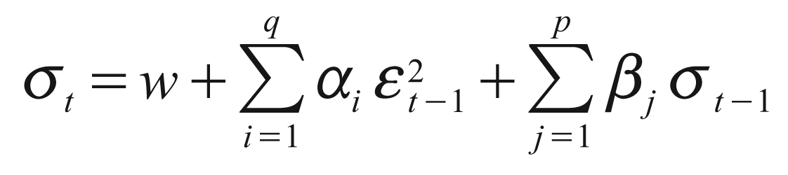
The (1, 1) in GARCH (1, 1) refers to the presence of a first-order autoregressive GARCH term (the first term in parentheses) and a first-order moving average ARCH term (the second term in parentheses) in the conditional variance equation. An ordinary ARCH model is a special case of a GARCH specification in which there are no lagged forecast variances.

The GARCH term model assumes that positive and negative shocks have the same effect on volatility because it depends on the square of the previous shocks. α (ARCH) is the ‘news’ coefficient with a higher value implying that recent news has a greater impact on price changes. It relates to the impact of yesterday’s news on today’s price changes. In contrast, β (GARCH) reflects the impact of ‘old news’ on price changes. It indicates the level of persistence in information and its effects on volatility.

Exponential GARCH Model

Nelson (1991) proposed EGARCH specification. It models the logarithm of the conditional variance and has an additional leverage term to capture asymmetry in volatility clustering. Unlike GARCH model, EGARCH model does not impose the non-negative constraints on the parameters. This model expresses the conditional variance of a given variable as a non-linear function of its own past values of standardized innovations that can react asymmetrically to good and bad news (Drimbetas et al., 2007).

The specification of conditional variance equation is expressed as:

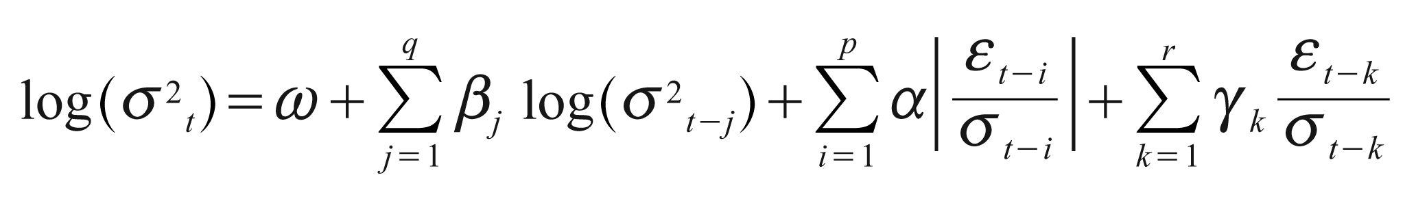
\log (σ_{}^{2}_{t}^{}) = ω + \sum_{j = 1}^{q} β_{j} \log (σ_{}^{2}_{t - j}^{}) + \sum_{i = 1}^{p} α | \frac{ε_{t - i}}{σ_{t - i}} | + \sum_{k = 1}^{r} γ_{k} \frac{ε_{t - k}}{σ_{t - k}}

(2)

In the model specification, β captures the volatility clustering effect, α measures the effect of news about volatility from the previous period on current period volatility and γ measures the leverage effect. The impact is asymmetric if γ ≠ 0. If γ = 0, positive and negative shocks have the same effect on volatility, while γ < 0 indicates that the bad news has a bigger impact on volatility than good news of same magnitude.

Threshold ARCH Model

Pioneered by Glosten et al. (1993), TARCH model incorporates a dichotomous variable to check whether there is statistically significant difference when shocks are negative. Unlike EGARCH model, the leverage effect is quadratic in TARCH model. The conditional variance can be represented as follows:

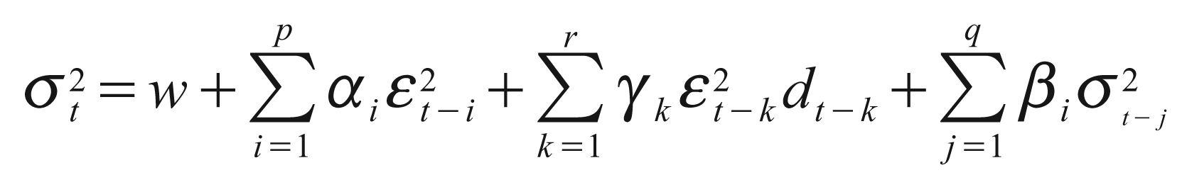
σ_{t}^{2} = w + {\sum^{​}}_{p}^{i = 1} α_{i} ε_{t - i}^{2} + {\sum^{​}}_{r}^{k = 1} γ_{k} ε_{t - k}^{2} d_{t - k} + {\sum^{​}}_{q}^{j = 1} β_{i} σ^{2}

(3)

where d_t = 1 if ε_t_{– j}< 0 and d_t = 0 otherwise. The parameter γ captures the asymmetrical effect of positive news and negative news. α and β are the ARCH and GARCH terms, respectively. Good news (ε_{t – j} < 0) and bad news (ε_{t – j} > 0) have differential impact on the conditional variance. Good news has an impact on α, while bad news has an impact on α + γ. If γ > 0, bad news increases volatility, and we say that there is a leverage effect for the ith order. The impact is asymmetric if γ ≠ 0 Negative γ estimates show that positive return shocks generate less volatility than negative shocks.

Power ARCH Model

Taylor (1986) and Schwert (1989) introduced the standard deviation GARCH model, where the standard deviation is modelled rather than the variance. This model, along with several other models, is generalized in Ding et al. (1993) with the power ARCH specification. In the power ARCH model, the power parameter δ of the standard deviation can be estimated rather than imposed, and the optional λ parameters are added to capture asymmetry of up to order τ. Variance equation in power ARCH (1, 1) is given by:

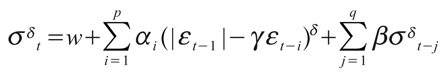
σ_{}^{δ}_{t}^{} = w + \sum_{i = 1}^{p} α_{i} {(| ε_{t - 1} | - γ ε_{t - i})}^{δ} + \sum_{j = 1}^{q} β σ^{δ}_{t - j}^{}

(4)

where α, β and γ are constant parameters and δ > 0 and | γ | < 1. Parameter δ can be fixed in the power ARCH model before estimation. Usually, choices for this parameter are δ = 1 (then the power ARCH model is robust to outliers) and δ = 2. Coefficient δ plays the role of a Box–Cox power transformation of the conditional standard deviation process. The power ARCH model embeds GARCH and its family models. For instance, when δ = 2 and δ = 0, power ARCH reduces to GARCH model. When δ = 2, power ARCH model reduces to an EGARCH model and it reduces to TARCH model when δ = 1.

Volatility Forecasts Indicators

The article employs a set of forecasting indicators to compare the predictive power of different forecasting models. These include root mean squared error (RMSE), mean absolute error (MAE), mean absolute percentage error (MAPE) and Theil’s inequality coefficient (TIC).

R M S E = \sqrt{\frac{1}{n} \sum_{t = 1}^{n} {({\hat{σ}}_{t} - σ_{t})}^{2}}

(5)

M A E = \frac{1}{n} \sum_{t = 1}^{n} | {\hat{σ}}_{t} - σ_{t} |

(6)

M A P E = \frac{1}{n} \sum_{t = 1}^{n} | ({\hat{σ}}_{t} - σ_{t}) / σ_{t} |

(7)

T I C = \frac{\sqrt{\frac{1}{n} {\sum^{​}}_{t = 1}^{n} {({\hat{σ}}_{t} - σ_{t})}^{2}}}{\sqrt{\frac{1}{n} {\sum^{​}}_{t = 1}^{n} {\hat{σ}}_{}^{2} + \frac{1}{n} {\sum^{​}}_{t = 1}^{n} σ_{}^{2}}}

(8)

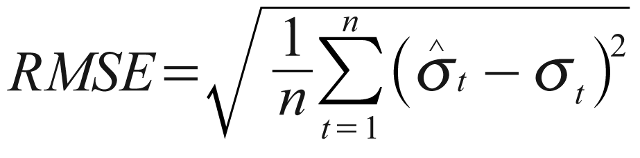
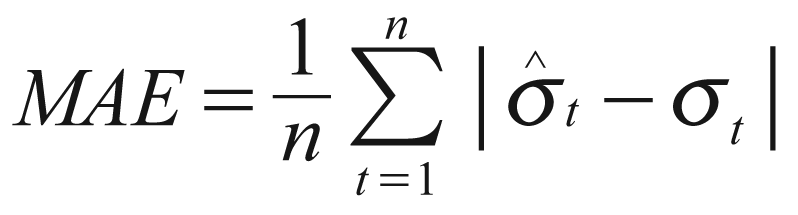
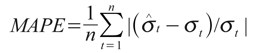
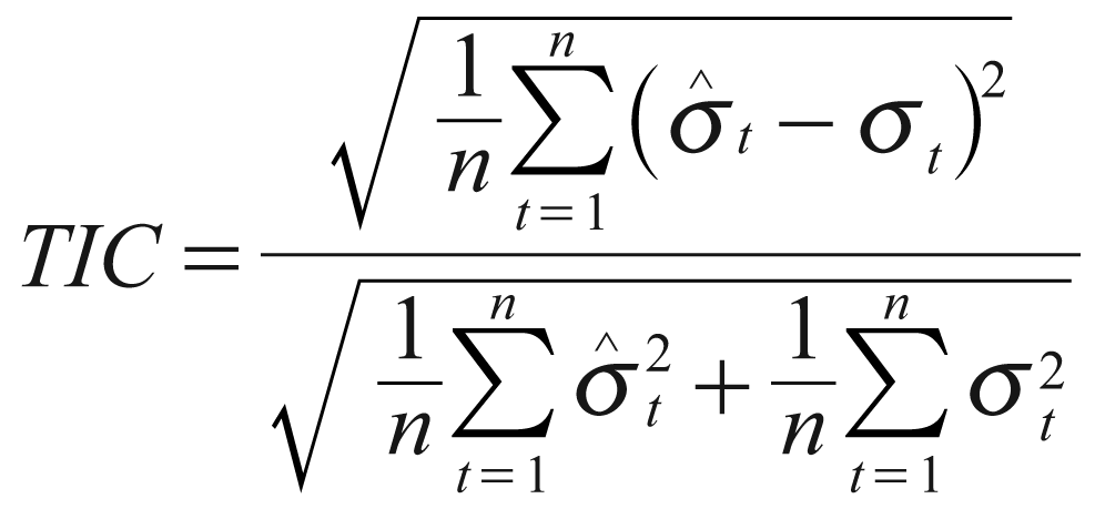
The first two forecast error statistics depend on the scale of the dependent variable. These are as relative measures to compare forecasts for the same series across different models; the smaller the error, the better the forecasting ability of that model according to that criterion. The remaining two statistics are scale invariant. The TIC always lies between zero and one, where zero indicates a perfect fit. In all the above cases ‘n’ stands for the number of out-of-sample forecasts, σ_t and ${\hat{σ}}_{t}$ represent the actual and forecasted volatility, respectively, at t.

Empirical Results

Preliminary Estimates

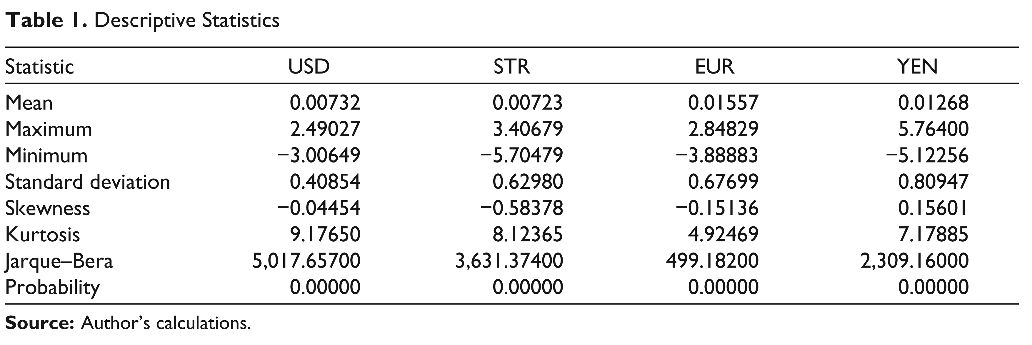
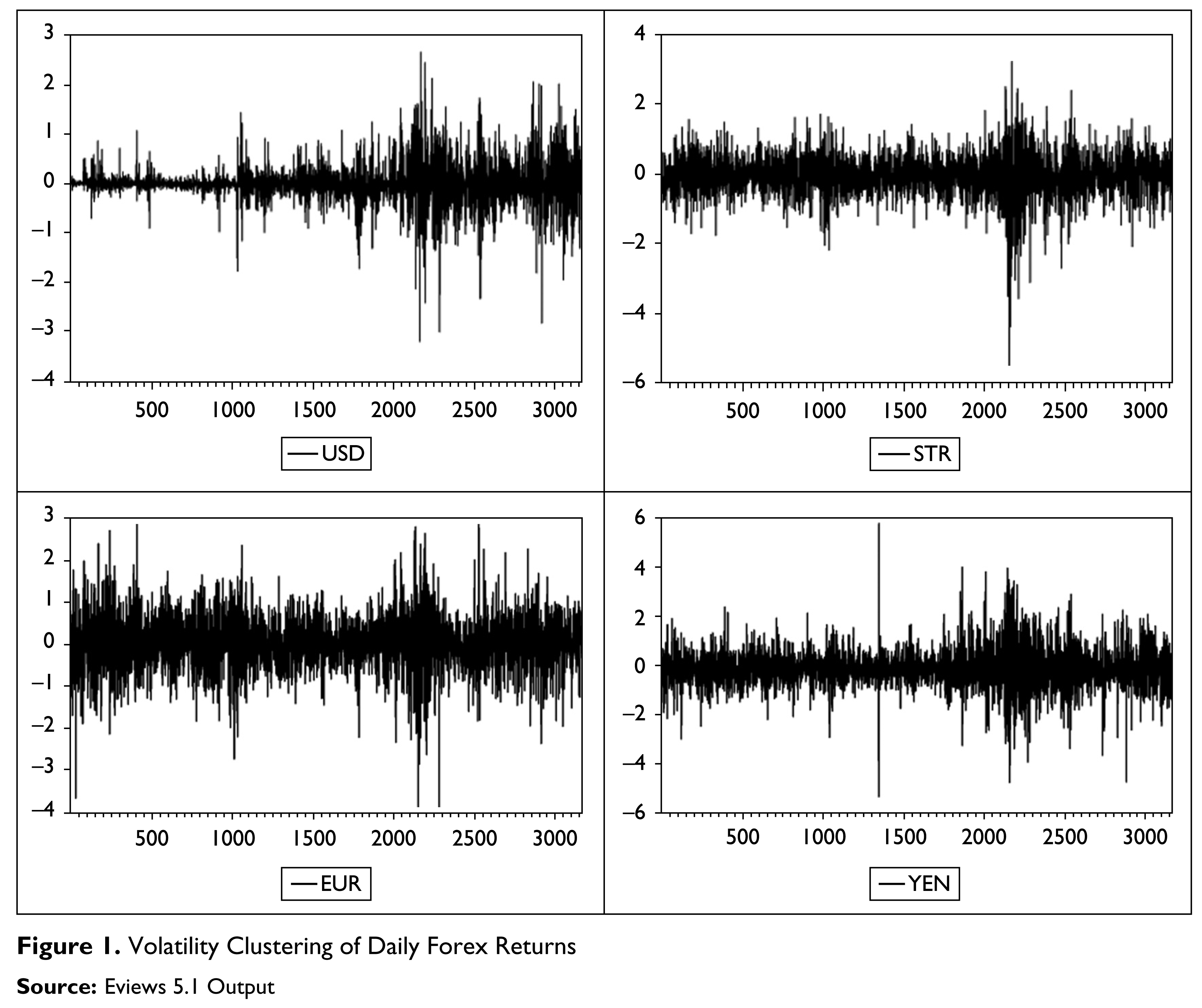
Table 1 presents the summary statistics of daily returns of four major currencies. The mean return was found to be highest in euro (0.01557) and Japanese yen (0.01268). The standard deviation in daily returns varied from 0.40854 to 0.80947. The statistics show that the return series is negatively skewed except for Japanese yen. The value of kurtosis is greater than 3 in all the return series, implying the fact that they have a heavier tail than the standard normal distribution. The daily forex returns are thus not normally distributed. Further, the significant Jarque–Bera statistics indicate departure from normality through rejecting the null hypothesis of symmetric distribution. Figure 1 displays the daily forex returns and exhibits the volatility clustering in the return series.

Table 1.

Descriptive Statistics

Statistic	USD	STR	EUR	YEN
Mean	0.00732	0.00723	0.01557	0.01268
Maximum	2.49027	3.40679	2.84829	5.76400
Minimum	−3.00649	−5.70479	−3.88883	−5.12256
Standard deviation	0.40854	0.62980	0.67699	0.80947
Skewness	−0.04454	−0.58378	−0.15136	0.15601
Kurtosis	9.17650	8.12365	4.92469	7.17885
Jarque–Bera	5,017.65700	3,631.37400	499.18200	2,309.16000
Probability	0.00000	0.00000	0.00000	0.00000

Source: Author’s calculations.

Testing of Stationarity

The viability of inference and forecasting of financial time series depend on their stationarity. A stationary return series will tend to return to its mean and fluctuations around its mean will have broadly constant amplitude. A stationary return series avoids the chances of spurious regression results.

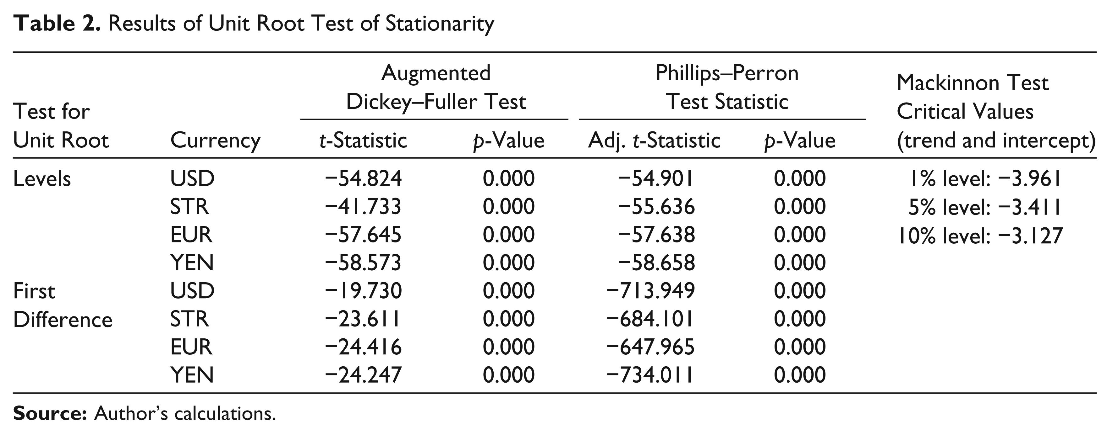
Unit root test tests the hypothesis of unit root against the alternative hypothesis of stationarity. ADF test and PP test are used in this study. The results of ADF and PP tests are given in Table 2. The analysis of the table indicates that the return series are stationary both at levels and on their first differences as their t-statistic is less than Mackinnon test critical value at 1, 5 and 10 per cent levels of significance.

Figure 1.

Source: Eviews 5.1 Output

Table 2.

Results of Unit Root Test of Stationarity

Test for Unit Root	Currency	Augmented Dickey–Fuller Test		Phillips–Perron Test Statistic		Mackinnon Test Critical Values (trend and intercept)
Test for Unit Root	Currency	t-Statistic	p-Value	Adj. t-Statistic	p-Value	Mackinnon Test Critical Values (trend and intercept)
Levels	USD	−54.824	0.000	−54.901	0.000	1% level: −3.961 5% level: −3.411 10% level: −3.127
	STR	−41.733	0.000	−55.636	0.000
	EUR	−57.645	0.000	−57.638	0.000
	YEN	−58.573	0.000	−58.658	0.000
First Difference	USD	−19.730	0.000	−713.949	0.000
	STR	−23.611	0.000	−684.101	0.000
	EUR	−24.416	0.000	−647.965	0.000
	YEN	−24.247	0.000	−734.011	0.000

Source: Author’s calculations.

Table 3.

GARCH (1, 1) Parameter Estimates

US Dollar
Parameter	Coefficient	Standard Error	z-Statistic	Probability	Residual Test Statistics
ω	0.0004	0.0000	9.0995	0.0000*	Q(15)	53.162*
					Q²(15)	32.050*
α_i	0.2906	0.0112	25.9856	0.0000*	ARCH-LM(5) Test	2.712*
					AIC	4.529
β_j	0.7709	0.0067	114.5831	0.0000*	SIC	4.541
					Log Likelihood	−7,128.1
Pound Sterling
ω	0.0047	0.0010	4.5388	0.0000*	Q(15)	13.479
					Q²(15)	31.015*
α_i	0.0447	0.0049	9.0611	0.0000*	ARCH-LM(5) Test	1.987***
					AIC	3.903
β_j	0.9424	0.0063	148.7583	0.0000*	SIC	3.915
					Log Likelihood	−6,141.4
Euro
ω	0.0035	0.0010	3.5447	0.0004*	Q(15)	7.285
					Q²(15)	10.318
α_i	0.0439	0.0050	8.8141	0.0000*	ARCH-LM(5) Test	0.589
					AIC	3.895
β_j	0.9487	0.0056	169.4463	0.0000*	SIC	3.906
					Log Likelihood	−6,128.0
Japanese Yen
ω	0.0209	0.0023	9.1866	0.0000*	Q(15)	22.071
					Q²(15)	22.227***
α_i	0.0992	0.0086	11.5616	0.0000*	ARCH-LM(5) Test	3.898*
					AIC	4.648
β_j	0.8681	0.0110	79.1780	0.0000*	SIC	4.660
					Log Likelihood	−7,315.3

Source: Author’s calculations.

Note: * significant at 1 per cent level, ** significant at 5 per cent level and *** significant at 10 per cent level.

GARCH (1, 1) Model

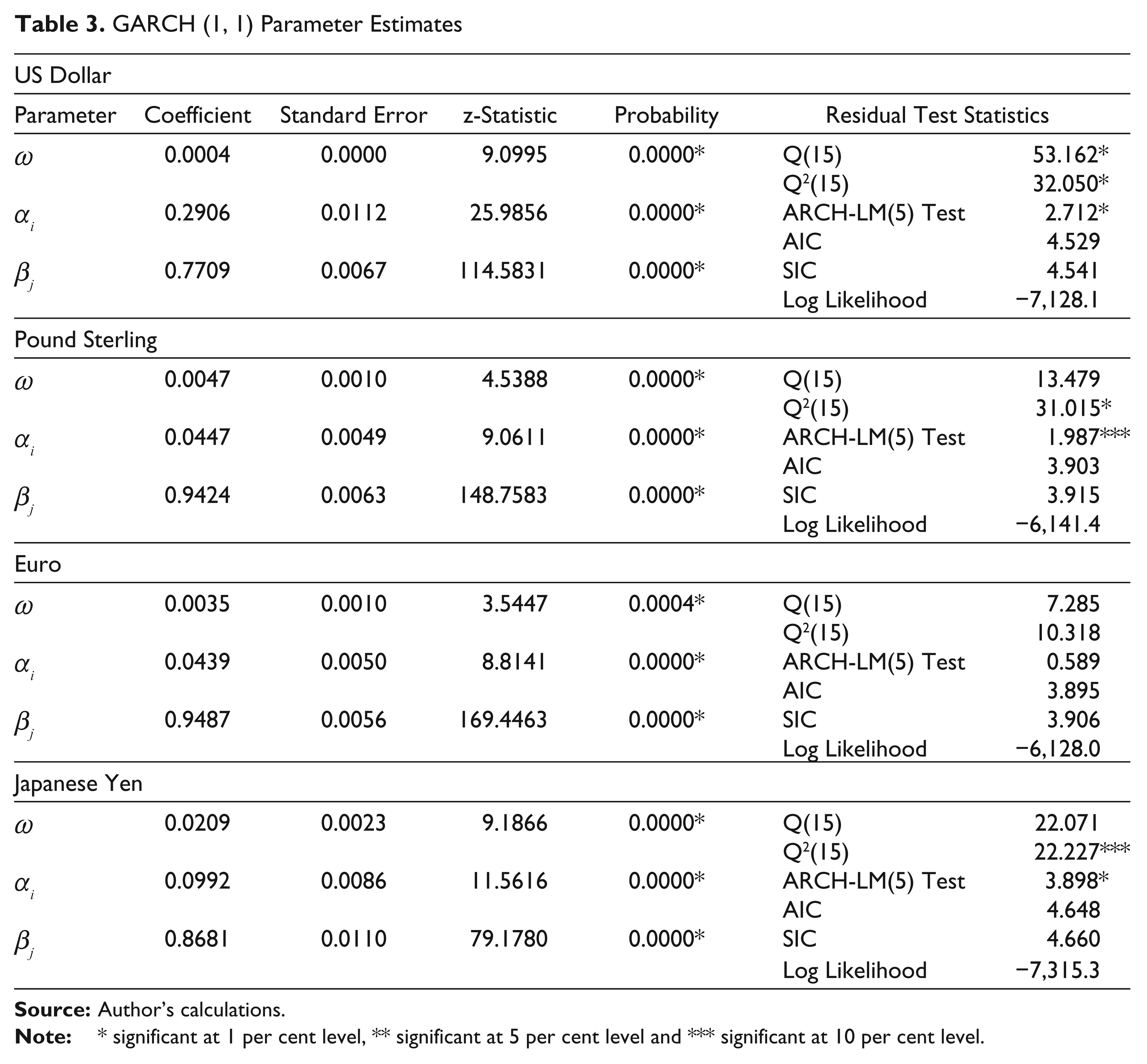
The results of GARCH (1, 1) model presented in Table 3 show that long-run volatility is given by the constant in the variance equation of GARCH specification between 0.0004 and 0.0209 per cent. The ARCH term capturing news about volatility from the previous period is 0.2906 (USD), 0.047 (STR), 0.0439 (EURO) and 0.092 (YEN). GARCH term which gives the last period forecast variance is on a higher side for all the return series suggesting that past conditional variance has a greater impact on volatility in forex returns than recent news announcements. It indicates the level of persistence in information and its effects on volatility. The sum of ARCH and GARCH coefficients is almost closer to one implying that shocks are persistent and the forecasts of conditional volatility take longer time to congregate to the stable level of variance.

EGARCH (1, 1) Model

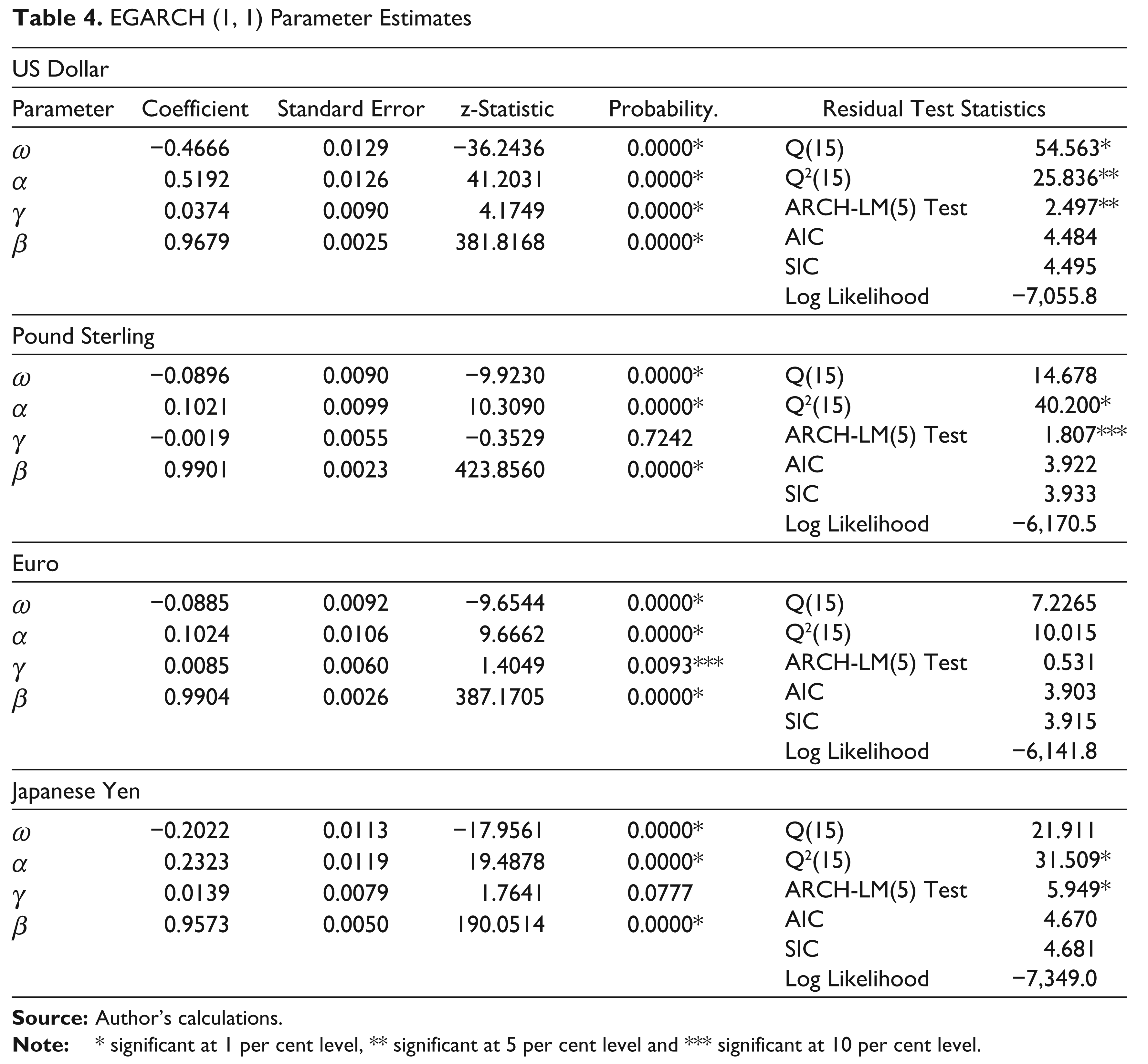
Table 4 exhibits the results of EGARCH (1, 1) model. All the currencies have posted positive and statistically significant beta coefficient suggesting volatility clustering. Positive beta signals that positive exchange rate changes are associated with further positive changes and vice versa. The impact of news about volatility from the previous period on current period volatility is also found to be significant at 1 per cent level for all the exchange rates. The results negate the existence of leverage effect and the news impact is asymmetric. Except for pound sterling, the gamma estimates were positive and statistically significant indicating that bad news has a smaller impact on volatility than good news of same magnitude.

Table 4.

EGARCH (1, 1) Parameter Estimates

US Dollar
Parameter	Coefficient	Standard Error	z-Statistic	Probability.	Residual Test Statistics
ω	−0.4666	0.0129	−36.2436	0.0000*	Q(15)Q²(15)ARCH-LM(5) TestAICSICLog Likelihood	54.56325.8362.497*4.4844.495−7,055.8
α	0.5192	0.0126	41.2031	0.0000*
γ	0.0374	0.0090	4.1749	0.0000*
β	0.9679	0.0025	381.8168	0.0000*
Pound Sterling
ω	−0.0896	0.0090	−9.9230	0.0000*	Q(15)Q²(15)ARCH-LM(5) TestAICSICLog Likelihood	14.67840.2001.807**3.9223.933−6,170.5
α	0.1021	0.0099	10.3090	0.0000*
γ	−0.0019	0.0055	−0.3529	0.7242
β	0.9901	0.0023	423.8560	0.0000*
Euro
ω	−0.0885	0.0092	−9.6544	0.0000*	Q(15)Q²(15)ARCH-LM(5) TestAICSICLog Likelihood	7.226510.0150.5313.9033.915−6,141.8
α	0.1024	0.0106	9.6662	0.0000*
γ	0.0085	0.0060	1.4049	0.0093***
β	0.9904	0.0026	387.1705	0.0000*
Japanese Yen
ω	−0.2022	0.0113	−17.9561	0.0000*	Q(15)Q²(15)ARCH-LM(5) TestAICSICLog Likelihood	21.91131.5095.9494.6704.681−7,349.0
α	0.2323	0.0119	19.4878	0.0000*
γ	0.0139	0.0079	1.7641	0.0777
β	0.9573	0.0050	190.0514	0.0000*

Source: Author’s calculations.

Note: * significant at 1 per cent level, ** significant at 5 per cent level and *** significant at 10 per cent level.

TARCH (1, 1) Model

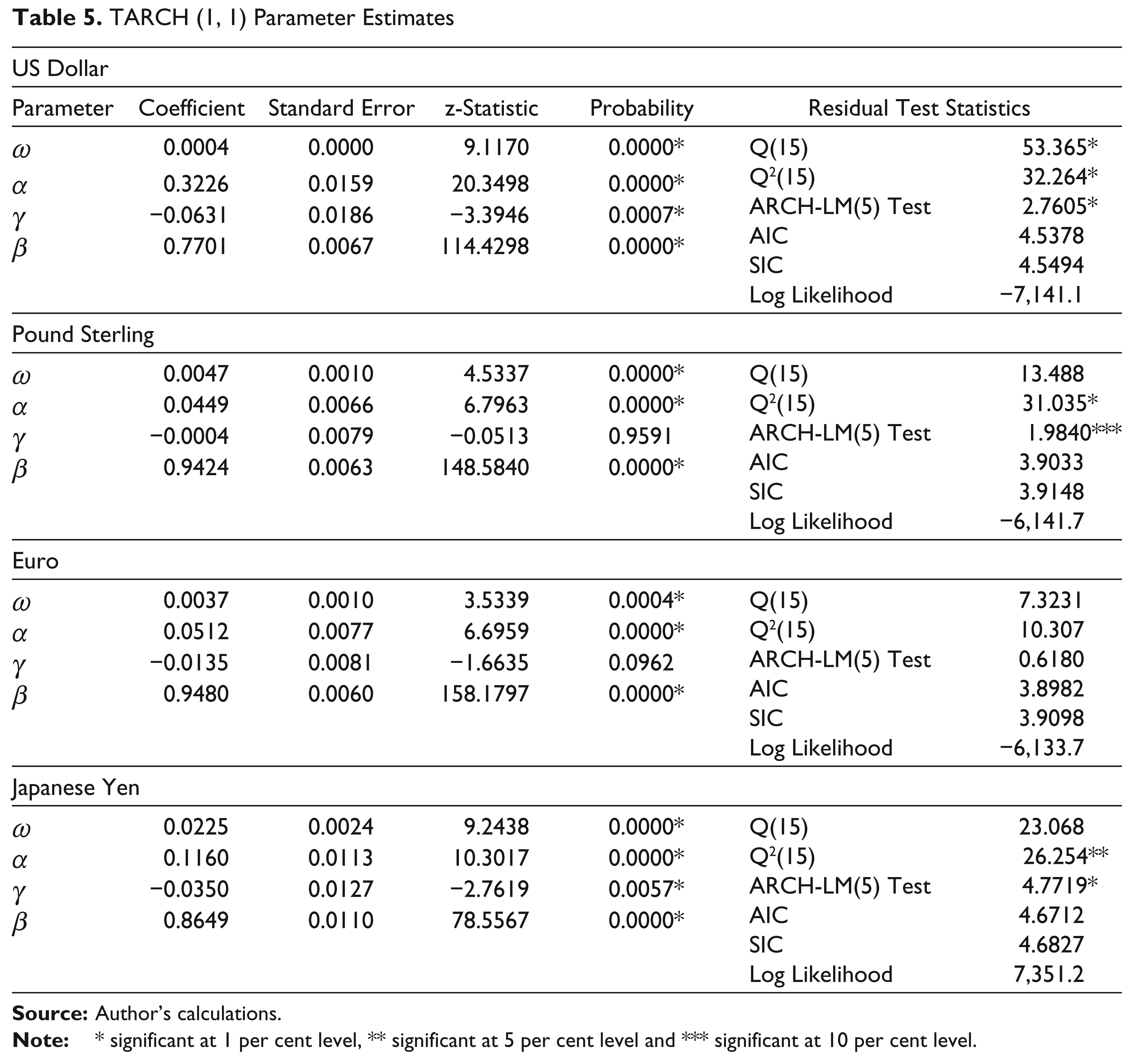
The results of TARCH model are given in Table 5. The γ coefficient is negative for all the return series indicating the absence of leverage effect in the return series of exchange rates, which means there is no tendency for negative innovations to generate greater volatility in future periods as compared with positive innovations of the same magnitude. The results show that good news has an impact of 0.3227, 0.0449, 0.0512 and 0.1160 magnitudes for USD, pound sterling, euro and Japanese yen, respectively. The impact of bad news as measured by α + β + γ/2 is highest for USD (1.061) followed by euro (0.9925), pound sterling (0.8699) and Japanese yen (0.8699) in that order. The leverage coefficients are statistically significant for USD and Japanese yen at 1 per cent level and for euro at 10 per cent level. The results further exhibit the persistence of shocks to volatility.

Table 5.

TARCH (1, 1) Parameter Estimates

US Dollar
Parameter	Coefficient	Standard Error	z-Statistic	Probability	Residual Test Statistics
ω	0.0004	0.0000	9.1170	0.0000*	Q(15)Q²(15)ARCH-LM(5) TestAICSICLog Likelihood	53.36532.2642.7605*4.53784.5494−7,141.1
α	0.3226	0.0159	20.3498	0.0000*
γ	−0.0631	0.0186	−3.3946	0.0007*
β	0.7701	0.0067	114.4298	0.0000*
Pound Sterling
ω	0.0047	0.0010	4.5337	0.0000*	Q(15)Q²(15)ARCH-LM(5) TestAICSICLog Likelihood	13.48831.0351.9840**3.90333.9148−6,141.7
α	0.0449	0.0066	6.7963	0.0000*
γ	−0.0004	0.0079	−0.0513	0.9591
β	0.9424	0.0063	148.5840	0.0000*
Euro
ω	0.0037	0.0010	3.5339	0.0004*	Q(15)Q²(15)ARCH-LM(5) TestAICSICLog Likelihood	7.323110.3070.61803.89823.9098−6,133.7
α	0.0512	0.0077	6.6959	0.0000*
γ	−0.0135	0.0081	−1.6635	0.0962
β	0.9480	0.0060	158.1797	0.0000*
Japanese Yen
ω	0.0225	0.0024	9.2438	0.0000*	Q(15)Q²(15)ARCH-LM(5) TestAICSICLog Likelihood	23.06826.254*4.77194.67124.68277,351.2
α	0.1160	0.0113	10.3017	0.0000*
γ	−0.0350	0.0127	−2.7619	0.0057*
β	0.8649	0.0110	78.5567	0.0000*

Source: Author’s calculations.

Note: * significant at 1 per cent level, ** significant at 5 per cent level and *** significant at 10 per cent level.

Power ARCH (1, 1) Model

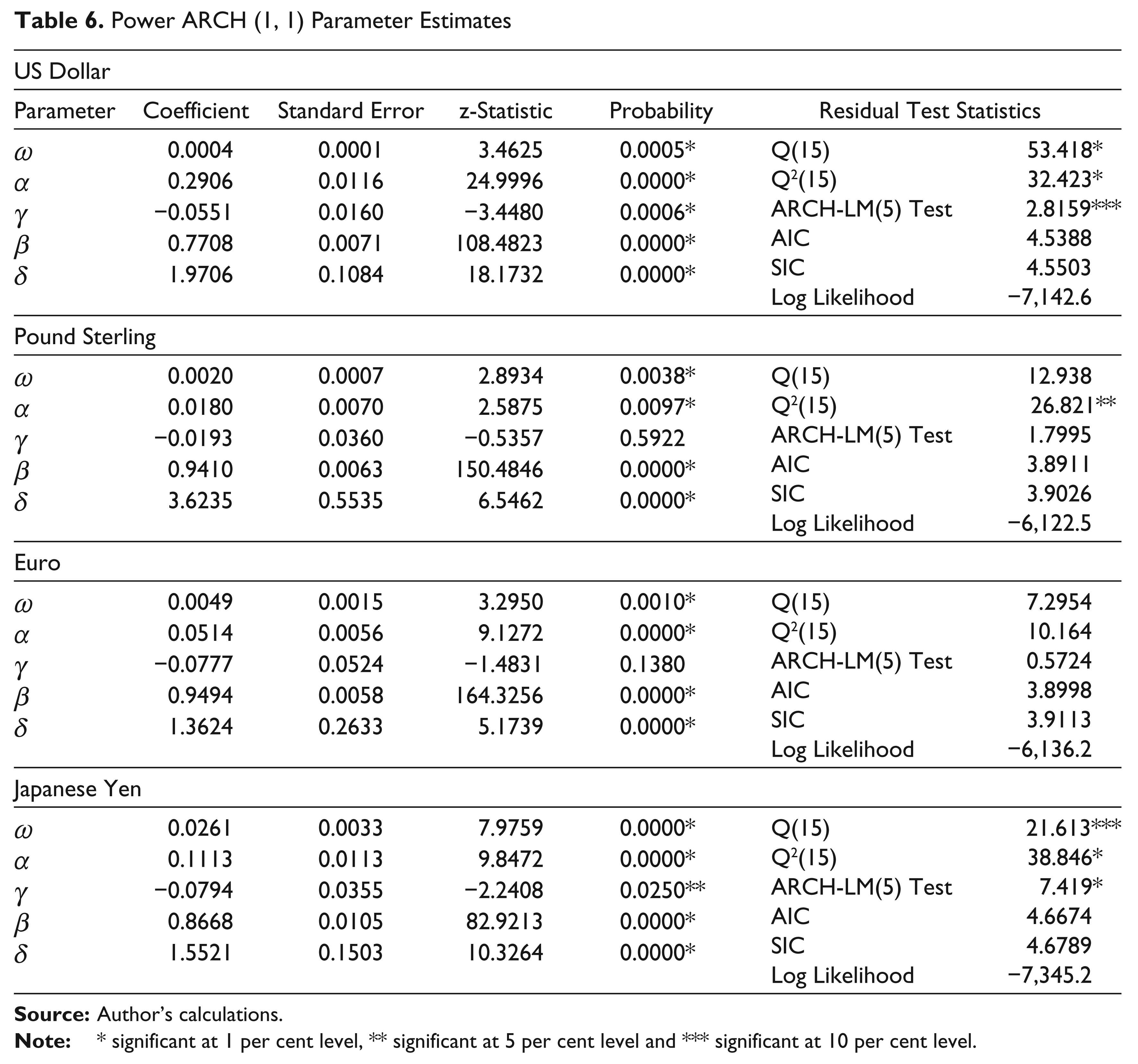
Table 6 shows the empirical results of power ARCH (1, 1) model. The term γ describes the existence of leverage effect or otherwise. Akin to the results of EGARCH (1, 1) and TGARCH (1, 1) models, negative γ coefficient for the return series shows the absence of leverage effect. The results suggest that good news has an impact of 0.2906, 0.0180, 0.0514 and 0.1112 for USD, pound sterling, euro and Japanese yen, respectively. The impact of bad news as measured by α + γ is highest for USD (0.1545) followed by Japanese yen (0.0317). The leverage coefficients are statistically significant for USD at 1 per cent, while other estimates failed to exhibit their statistical significance. Further, the study reported that the power parameter δ was less than 2 for all the return series except for pound sterling.

Table 6.

Power ARCH (1, 1) Parameter Estimates

US Dollar
Parameter	Coefficient	Standard Error	z-Statistic	Probability	Residual Test Statistics
ω	0.0004	0.0001	3.4625	0.0005*	Q(15)Q²(15)ARCH-LM(5) TestAICSICLog Likelihood	53.41832.4232.8159***4.53884.5503−7,142.6
α	0.2906	0.0116	24.9996	0.0000*
γ	−0.0551	0.0160	−3.4480	0.0006*
β	0.7708	0.0071	108.4823	0.0000*
δ	1.9706	0.1084	18.1732	0.0000*
Pound Sterling
ω	0.0020	0.0007	2.8934	0.0038*	Q(15)Q²(15)ARCH-LM(5) TestAICSICLog Likelihood	12.93826.821**1.79953.89113.9026−6,122.5
α	0.0180	0.0070	2.5875	0.0097*
γ	−0.0193	0.0360	−0.5357	0.5922
β	0.9410	0.0063	150.4846	0.0000*
δ	3.6235	0.5535	6.5462	0.0000*
Euro
ω	0.0049	0.0015	3.2950	0.0010*	Q(15)Q²(15)ARCH-LM(5) TestAICSICLog Likelihood	7.295410.1640.57243.89983.9113−6,136.2
α	0.0514	0.0056	9.1272	0.0000*
γ	−0.0777	0.0524	−1.4831	0.1380
β	0.9494	0.0058	164.3256	0.0000*
δ	1.3624	0.2633	5.1739	0.0000*
Japanese Yen
ω	0.0261	0.0033	7.9759	0.0000*	Q(15)Q²(15)ARCH-LM(5) TestAICSICLog Likelihood	21.613**38.8467.419*4.66744.6789−7,345.2
α	0.1113	0.0113	9.8472	0.0000*
γ	−0.0794	0.0355	−2.2408	0.0250**
β	0.8668	0.0105	82.9213	0.0000*
δ	1.5521	0.1503	10.3264	0.0000*

Source: Author’s calculations.

Note: * significant at 1 per cent level, ** significant at 5 per cent level and *** significant at 10 per cent level.

Forecasts of Volatility

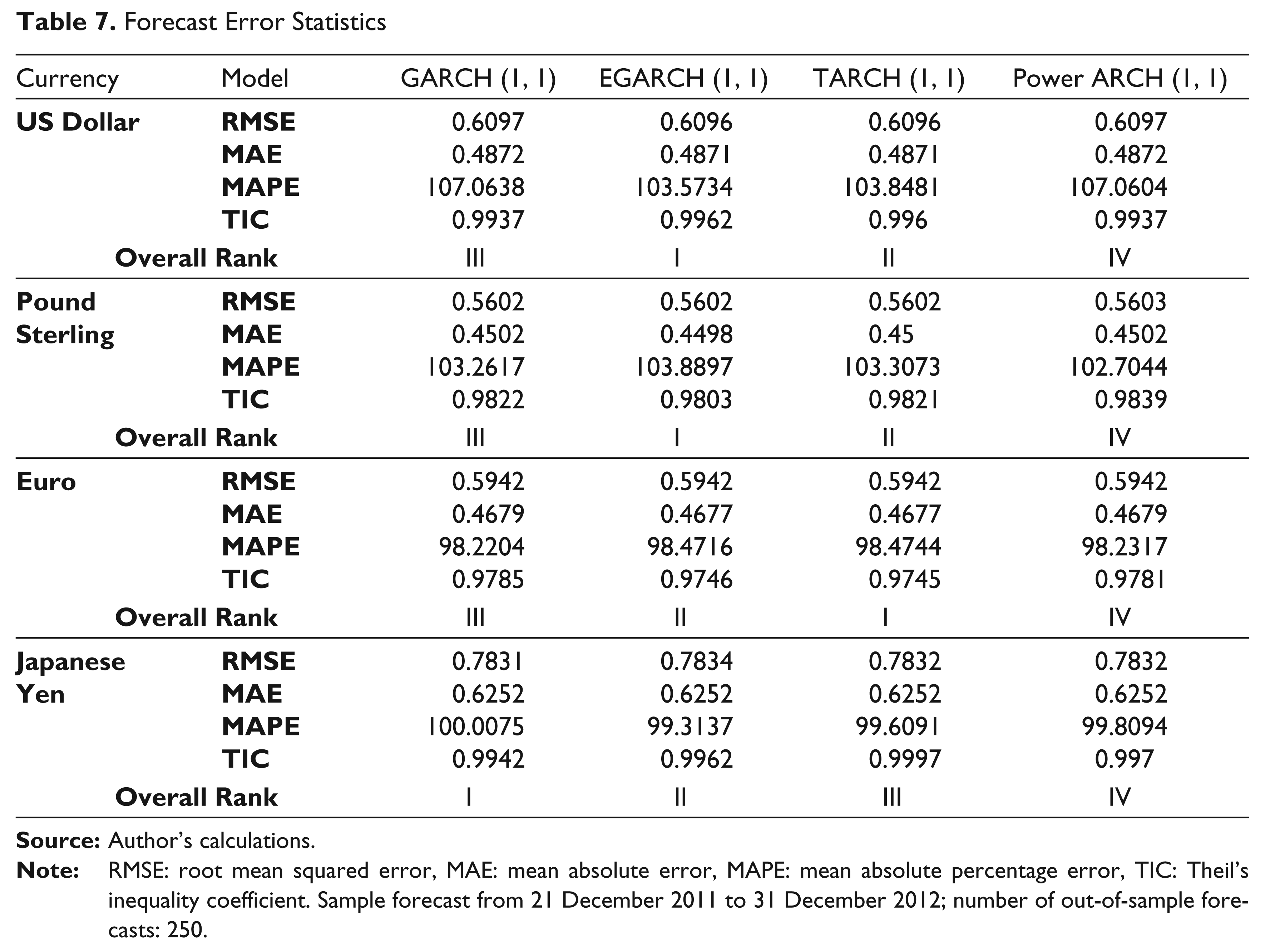
Table 7 shows the results of out-of-sample forecast performance of the estimated models. The model that reports the lowest values of the error statistic is considered to be the best model. The results show that the EGARCH (1, 1) model outperformed all the other models in forecasting the volatility of USD and pound sterling. TARCH (1, 1) model and GARCH (1, 1) model fared better in predicting volatility of euro and Japanese yen, respectively. The forecast errors are very close for all the models.

Table 7.

Forecast Error Statistics

Currency	Model	GARCH (1, 1)	EGARCH (1, 1)	TARCH (1, 1)	Power ARCH (1, 1)
US Dollar	RMSE	0.6097	0.6096	0.6096	0.6097
	MAE	0.4872	0.4871	0.4871	0.4872
	MAPE	107.0638	103.5734	103.8481	107.0604
	TIC	0.9937	0.9962	0.996	0.9937
	Overall Rank	III	I	II	IV
Pound Sterling	RMSE	0.5602	0.5602	0.5602	0.5603
	MAE	0.4502	0.4498	0.45	0.4502
	MAPE	103.2617	103.8897	103.3073	102.7044
	TIC	0.9822	0.9803	0.9821	0.9839
	Overall Rank	III	I	II	IV
Euro	RMSE	0.5942	0.5942	0.5942	0.5942
	MAE	0.4679	0.4677	0.4677	0.4679
	MAPE	98.2204	98.4716	98.4744	98.2317
	TIC	0.9785	0.9746	0.9745	0.9781
	Overall Rank	III	II	I	IV
Japanese Yen	RMSE	0.7831	0.7834	0.7832	0.7832
	MAE	0.6252	0.6252	0.6252	0.6252
	MAPE	100.0075	99.3137	99.6091	99.8094
	TIC	0.9942	0.9962	0.9997	0.997
	Overall Rank	I	II	III	IV

Source: Author’s calculations.

Note: RMSE: root mean squared error, MAE: mean absolute error, MAPE: mean absolute percentage error, TIC: Theil’s inequality coefficient. Sample forecast from 21 December 2011 to 31 December 2012; number of out-of-sample forecasts: 250.

Conclusion

This article examines the existence of volatility clustering and leverage effect in the Indian forex market over the period from January 2000 to December 2012. GARCH, EGARCH, TARCH and power ARCH models were used in this context to determine the patterns of volatility. The mean return was found to be highest in euro (0.01557) and Japanese yen (0.01268). The daily forex returns were not normally distributed. The return series display the phenomenon of volatility clustering. The results indicated that past conditional variance has a greater impact on volatility in forex returns than recent news announcements. No significant leverage effects were evident. Volatility seems to be persistent in nature. Given the high volatile nature of the capital markets, the studies on volatility patterns would definitely help in diversification of portfolios and enable the traders to take hedge positions to shield their investments.

References

Abdalla

I.S.

, & Murinde

(1997). Exchange rate and stock price interactions in emerging financial markets: Evidence on India, Korea, Pakistan and the Philippines. Applied Financial Economics, 7(1), 25–35.

Akgiray

(1989). Conditional heteroscedasticity in time series of stock returns: Evidence and forecast. Journal of Business, 62(1), 55–80.

Andersen

T.G.

, & Bollerslev

(1998). Answering the skeptics: Yes, standard volatility models do provide accurate forecasts. International Economic Review, 39(4), 885–905.

Aydemir

, & Demirhan

(2009). The Relationship between Stock Prices and Exchange Rates Evidence from Turkey. International Research Journal of Finance and Economics, 23, 207–215.

Beer

, & Hebein

(2008). An assessment of the stock market and exchange rate dynamics in industrialized and emerging markets. International Business and Economics Research Journal, 7(8), 59–70.

Bhanumurthy

N.R.

(2004). Macroeconomic fundamentals and exchange rate dynamics in India: Some survey results. Economic and Political Weekly, 41(11), 1101–1107.

Black

(1976). Studies in stock price volatility changes. Proceedings of the 1976 Business Meeting of the Business and Economics Statistics Section, American Statistical Association, pp. 177–181.

Bollerslev

(1986). Generalized Autoregressive Conditional Heteroskedasticity. Journal of Econometrics, 31(3), 307–27.

Brailsford

T.J.

, & Faff

R.W.

(1996). An evaluation of volatility forecasting techniques. Journal of Banking and Finance, 20(3), 419–438.

10.

Brooks

(1998). Predicting stock index volatility: Can market volume help? Journal of Forecasting, 17(1), 59–80.

11.

Chan

, & Fung

(2007). Forecasting volatility of Hang Seng Index and its application on reversing for investment guarantees. Working Paper, The Actuarial Society of Hong Kong.

12.

Chang

H.L.

, Su

C.W.

, & Lai

Y.C.

(2009). Asymmetric price transmissions between the exchange rate and stock market in Vietnam. International Research Journal of Finance and Economics, 23, 104–113.

13.

Corhay

, & Rad

(1994). Statistical properties of daily returns: Evidence from European stock markets. Journal of Business Finance and Accounting, 21(2), 271–282.

14.

De Grauwe

, & Markiewicz

(2013). Learning to forecast the exchange rate: Two competing approaches. Journal of International Money and Finance, doi: 10.1016/ j.jimonfin.2012.03.001

15.

Dibooglu

, & Kutan

A.M.

(2001). Sources of Real Exchange Rate Fluctuations in Transition Economies: The Case of Poland and Hungary. Journal of Comparative Economics, 29(2), 257–275.

16.

Ding

, Engle

R.F.

, & Granger

C.W.J.

(1993). Long Memory Properties of Stock Market Returns and a New Model. Journal of Empirical Finance, 1(1), 83–106.

17.

Drimbetas

, Sariannidis

, & Porfiris

(2007). The effect of derivatives trading on volatility of the underlying asset: evidence from the Greek stock market. Applied Financial Economics, 17(2), 139–148.

18.

Duan

J.C.

, & Zhang

(2001). Pricing hang send index options around the Asian financial crisis—A GARCH approach. Journal of Banking and Finance, 25(11), 1989–2014.

19.

Flood, & Rose. (1995). Fixed Exchange Rates: A Virtual Quest for Fundamentals. Journal of Monetary Economics, 36(1), 3–37.

20.

Glosten

Lawrence R.

, Jagannathan

, & Runkle

D.E.

(1993). On the Relation between the Expected Value and the Volatility of the Nominal Excess Returns on Stocks. Journal of Finance, 48(5), 1779–1791.

21.

Hsing

(2011). Analysis of exchange rate fluctuations in Poland: Test of the interest parity condition. Journal of Transition Economics and Finance, 1, 24–28.

22.

Kamal

, Haq

H.U.

, Ghani

, & Khan

M.M.

(2012). Modeling the exchange rate volatility, using generalized autoregressive conditionally heteroscedastic (GARCH) type models: Evidence from Pakistan. African Journal of Business Management, 6(8), 2830–2838.

23.

Karmakar

(2005). Modeling conditional volatility in the Indian stock markets. Vikalpa, 30(3), 21–37.

24.

Kumar

, & Dhankar

R.S.

(2010). Empirical analysis of conditional heteroskedasticity in time series of stock returns and asymmetric effect on volatility. Global Business Review, 11(1), 21–33.

25.

Kumar

S.S.S.

(2006). Forecasting volatility—Evidence from Indian stock and forex markets. IIMK/WPS/08/FIN/ 2006/06.

26.

Lee

K.Y.

(1991). Are the GARCH Models Best in out of Sample Performance? Economics Letter, 37(3) 305–308.

27.

McMillan

D.G.

, Speight

A.E.H.

, & Ap Gwilym

(2000). Forecasting UK stock market volatility. Applied Financial Economics, 10(4), 435–448.

28.

Mishra

A.K.

(2004). Stock market and foreign exchange market in India. South Asia Economic Journal, 5(2), 209–232.

29.

Mondal

(2012). Foreign exchange market intervention and exchange rate volatility: A bivariate GARCH model for India. The IUP Journal of Bank Management, 11(4), 29–40.

30.

Nelson

D.B.

(1991). Conditional Heteroscedasticity in Asset Returns: A New Approach. Econometrica, 59(2), 347–70.

31.

Pagan

, & Schwert

G.W.

(1990). Alternative models for conditional stock volatilities. Journal of Econometrics, 45(1/2), 267–290.

32.

Rashid

, & Ahmad

(2008). Predicting Stock Returns Volatility: An Evaluation of Linear vs. Nonlinear Methods, International Research Journal of Finance and Economics, 20, 141–150.

33.

Ray

(2012). A bivariate exploration into stock prices and exchange rate dynamics in selected Asian economies. International Journal of Contemporary Business Studies, 3(3), 43–59.

34.

Schwert

(1989). Stock Volatility and Crash of 87. Review of Financial Studies, 3(1), 77–102.

35.

Shehu

A.A.

, & Youtang

(2012). Exchange rate volatility, trade flows and economic growth in a small open economy. International Review of Business Research Papers, 8(2), 118–131.

36.

Siddharth

, & Vinod

(2012, July 31). Depreciating rupee—Causes, impacts and actions. Retrieved 16 March 2013, from http://www.managementcanvas.iimindore.in

37.

Srikanth

, & Kishor

(2012). Exchange rate dynamics in Indian foreign exchange market: An empirical investigation on the movement of USD/INR. The IUP Journal of Applied Finance, 18(4), 46–61.

38.

Srinivasan

, & Ibrahim

(2010). Forecasting stock market volatility of BSE 30 index using Garch Models. Asia-Pacific Journal of Management Research and Innovation, 6(3), 47–60.

39.

Taylor

S.J.

(1986) Modeling Financial Time Series. Chichester, UK: John Wiley and Sons.

40.

Tripathy

, & Gil-Alana

L.A.

(2010). Suitability of volatility models for forecasting stock market returns: A study on the Indian national stock exchange. American Journal of Applied Sciences, 7(11), 1487–1494.